Nucleus: Towards a Unified Dynamics Solver for Computer Graphics
←
→
Page content transcription
If your browser does not render page correctly, please read the page content below
Nucleus: Towards a Unified Dynamics Solver for Computer Graphics

                                                     Jos Stam
                                                   Autodesk, Inc.
                                              Jos.Stam@autodesk.com

                        Abstract                             be problematic. In this paper we present a solver that
                                                             tries to resolve these interactions simultaneously.
   This paper presents a unified dynamics solver                 We describe both how we model different shapes of
developed by the author which was first released in          matter and how we simulate them. We decided to use a
Autodesk™ MAYA 8.5. The solver however is a                  simplicial complex as our shape model as it includes
standalone library which could potentially be used in        points, curves, surfaces and solids in a unified
other applications. Current dynamics solvers are             framework. For the simulation part we use a space-
usually fine tuned for specific effects such as rigid        time based approach for the collisions and a constraint
bodies or cloth. Handling the interaction between these      based approach to account for deformations. This
solvers is often problematic as one of them takes            approach results in simulations that are relatively stable
precedence over the others. In our Nucleus solver we         for stiff materials such as cloth.
model all matter as a simplicial complex: a                      By allowing various elements of matter to interact
generalization of a triangle mesh that also includes         in this manner we get interesting emergent behaviors.
points, curves and solids. This allows interactions such     Even though each interaction is simple more complex
as collisions between various elements of different          behaviors emerge. For example a flapping flag can be
dimensionality. The internal deformations such as            simulated using a simple directional wind field and an
stretch and bend are handled through constraints             inextensible piece of cloth. The flapping behavior
instead of springs. This makes the simulation more           emerges from the drag and lift constraints battling the
stable for stiff materials such as cloth. Through mutual     stretch constraint. The behavior emerges without the
interactions and constraints many interesting                need for a complicated air flow model. Throughout our
phenomena emerge automatically. The basic                    research we emphasize simplicity as it vastly reduces
philosophy behind Nucleus is that complexity arises by       the amount of code and consequently the amount of
combining simple constraints.                                potential bugs. This is not just an aesthetic bias on our
                                                             part rooted in a desire to achieve mathematical
   1. Introduction                                           elegance. In practice adhering to this principle results
                                                             in more robust and stable commercial products.
   The convincing simulation of interacting
deformable objects is hard to achieve using traditional        2. Previous and Related Work and the
animation techniques such as key-framing alone.              History of Nucleus
Therefore there is a need in computer graphics to rely
on physics-based dynamics solvers. Instead of                   Simulations based on physics are evidently not
specifying exact poses through key frames an animator        novel in computer graphics. This approach was
specifies material properties of the object’s and            pioneered in the late eighties by many researchers [18].
external forces. Given this information the dynamics         Early work focused mainly on spring-based models for
solver then ideally computes snapshots of the states of      deformable matter and used either explicit or implicit
all the objects over fixed time-steps. Most current          methods. In addition many works have focused on
solvers are fine tuned for a specific effect such as rigid   simulating rigid bodies [5,13,17]. As far as we know
bodies and cloth. Resolving interactions between such        the first paper to handle deformations as constraints
solvers can become problematic. For example, imagine         was Provot’s strain limiting procedure used for cloth
a rigid body like a soccer ball being kicked in a goal.      [16], see also [9] and the pioneering work of Moreau
There will be a two way interaction between the ball         [14]. Since then others have used this approach [12,15]
and the net. Achieving this effect by connecting a rigid     to good use. Recently this approach seems to gain
body solver to a curve-based solver for the goal net can     acceptance in academia as well [10].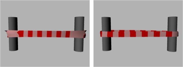
The system closest in spirit to ours is the position     meager 100 files versus the 40,000 or so files
based dynamics work of Müller et al. [15] developed          populating the MAYA code base.
independently from us and the collision work by                 The capabilities of the new solver were first
Bridson et al. [6]. We do not cover here in detail the       demonstrated at Autodesk’s user’s group at
vast literature on this subject but only cite work that      SIGGRAPH 2006 by Duncan Brinsmead in Boston in
directly inspired us or is closely related. We refer the     July and later in a key note talk by the author at
reader instead to one of the many surveys on this topic      EUROGRAPHICS 2006 in September in Vienna. The
and the references in the papers cited. The goal of this     solver was first released in early 2007 in Autodesk™
paper is to give an overview of the ideas and                MAYA 8.5 Unlimited with the release of nCloth. This
techniques that were implemented in the Nucleus              release only exposed the cloth capabilities. In 2008 we
library.                                                     released an nParticle feature allowing the interaction
    Research on the Nucleus solver started as a small        between particles and nCloth objects. We are hoping to
project by the author of this paper in the fall of 2000 in   add many more features in the future and enhance the
Seattle to create a very simple cloth solver for a cool      Nucleus solver.
live demo of smoke interacting with cloth. The idea
was to replace springs with hard links. Since cloth is          3. Shape Model: Simplicial Complexes
not stretchy it seemed like a bad idea to use very stiff
springs to model it. So instead we started with hard            Since we are interested in modeling a whole range
links treated like constraints. Stiff springs have several   of shapes in a unified manner we decided to use the
problems. Explicit integrators require small time steps      theory of simplicial complexes. It is a well known fact
to achieve stability which result in long simulation         that any surface can be approximated by a triangular
times. On the other hand stable implicit time                mesh to any arbitrary precision. A generalization of
integration schemes damp out off spring motion which         this result is a theorem first proved by Brouwer in 1910
results in overly damped animations. We will make            which loosely states that “Every continuous mapping
these points more concrete in a simple setting below.        can be approximated by a piece-wise linear simplicial
    The system we implemented initially was so simple        map.” Or more precisely in math-speak:
that we wrote a version for the Palm just for fun back
in 2001 for a very small 8x8 piece of cloth, followed                      :
by an implementation on the PocketPC with variable              Let and be complexes; let be finite.
resolution. Both demos were “beamed” around at that             Given a continuous map    | | | |
time. We also showed a demo of cloth interacting with           there is an such that has a simplicial
smoke in the “Visual Simulation of Smoke” paper                 approximation     sd : K → L.
presentation at SIGGRAPH in Los Angeles in 2001.
    But it wasn’t until the author of this paper showed         For our purposes it is sufficient to define a
the demos at the SIGGRAPH 2003 annual                        simplicial complex as an assemblage of simplices. A
Alias|wavefront’s user’s group in San Diego that some        simplex is a generalization of a triangle to any
buzz was generated amongst our user base.                    dimension. Figure 1 shows four different k-simplices
Subsequently we were asked by upper management at            that model points, edges, triangles and tetrahedra.
Alias|wavefront to replace the existing cloth solver in      More complicated shapes are modeled by gluing these
MAYA with our new one.                                       building blocks together. The blocks do not need to
    This task was quite a challenge since the existing       have the same dimension as shown in Figure 2. The
cloth solver in MAYA was pretty sophisticated. Soon          definition of a simplicial complex is purely topological
after we got seriously involved in this project we           as it establishes a relationship between elements of an
realized that our framework could accommodate other          arbitrary set. The latter can be points in space, masses,
elements than cloth. That happened somewhere in the          colors, etc. We therefore neatly separate the topology
summer of 2004 and that was when the concept of a            from the geometry. In practice our implementation of
Nucleus solver really took off. After that we wrote          the simplicial complex code contains only ints and no
many prototypes and the final version of the solver was      floats for example.
written in the (hot) fall and (early) winter of 2005 in
Toronto, Canada. It was then further refined and
integrated into MAYA during 2006.
    We made sure to build an API around our solver
such that any changes at a low level would not affect
function calls on the MAYA side. Our Nucleus solver
                                                                Figure 1: four k-simplices.
is tiny compared to the MAYA source code: about a
4. Dynamics

                                                               4.1. Basic Equations

                                                               The dynamics of a simplicial complex is defined by
                                                            the motion of its N vertices. We can compact this
   Figure 2: Two examples of a simplicial complex.
                                                            description in a 3N vector:
   The neat aspect of using a unified model for the
shapes is that it leads to a very elegant implementation                                   ,…,        .
using only a single data structure:
                                                               The particles evolve due to external forces and
   class simplex {                                          internal deformations defined by the simplices and
      int k;                                                other factors as explained below. The laws that govern
      int sign;                                             the motion of the particles are well known since
      int vertex[k+1];                                      Newton stated them in his famous Principia in 1687.
      int child[k+1];                                       In particular his second law states that (assuming unit
      int n_parents;                                        masses):
      int parent[n_parents];
   };
                                                                                       0
    For each simplex we store its dimension k. We also                                 0
store the k+1 indices of the elements and the k+1 (k-1)-
simplices that it contains. For example a 2-simplex         where         is the internal energy due to deformations
(triangle) contains 3 1-simplices (edges). A simplex        and      model external forces like gravity. The initial
can have an arbitrary number of parents. For example,       state is defined by the initial positions and velocities of
a point (0-simplex) in a mesh can have an arbitrary         the particles. An alternative way to specify the
number of incident edges (1-simplices). In this case the    dynamics is to require that the particles minimize the
number of parents of the point is commonly called its       total energy at each instant of time:
valence. We also store a sign for each simplex for the
following reason. For many operations it helps if the                          1
indices of the elements are stored in lexicographical                            | |                  ·
                                                                               2
order. However, this rearrangement of the indices can
change the orientation of the simplex. When the                 The first term is the total kinetic energy, the second
number of transpositions is odd the sign is -1 otherwise    term is the potential energy and the last term is the
it is 1. A zero sign value indicates that the element       work done by the external forces. A very good
does not have an orientation. The sign also allows          introduction from a mathematical point of view is the
many algebraic operations to be simplified on               monograph by Arnold [3]. These equations have been
simplices.                                                  around for over 300 years and one would expect that
    In this paper we will not get into all the details of   there is a standard numerical procedure to solve them.
implementing operations on simplical complexes.             However, this is not the case and to understand the
However, the above data structure allows us to              difficulties we turn to a simple problem in more detail.
implement many queries effortlessly that are needed to
set up the constraints described below.                        4.2. On the Motion of a Simple Spring
    We encourage the reader who is interested in
learning more about this topic to consult the excellent        It is interesting that even the problem of solving the
introduction to this topic by Alexandrov [1]. Also we       dynamics of a simple linear spring exhibits the
recommend his more detailed monograph which has             behavior and difficulties common to more
proven to be very helpful [2]. Both books are also very     sophisticated solvers. This section is not a thorough
affordable because they have been cheaply reprinted by      overview of numerical integrators. For a good review
Dover publication.                                          see the excellent book by the group from my alma
                                                            mater at l’Université de Genève [11]. The intent here is
                                                            to focus on one of the simplest problems and
                                                            understand the basic numerical problems one can
                                                            encounter.
The equations for a linear spring are
0
0 0 .
To visualize the motion of the spring we can draw
its trajectory in the phase space , , a plane in this
case. From the conservation of energy:
Figure 4: Trajectory of the spring is tangent to the
1 1 1 1 vector field.
2 2 2 2
we know that the trajectories are circles in the phase We now analyze three methods to solve this
plane whose radius is a function of the initial state as equation numerically with a fixed time step . The
shown in Figure 3. The equation can also be computed time derivative between two consecutive states is
analytically in this case. There is an elegant way to approximated by:
obtain this result by introducing the complex number
. In this manner the equation for the motion
.
of the spring reduces to an ordinary differential
equation:
In an explicit scheme the right hand side of the
equation is evaluated at the current state, so that
0
1 .
Whose solution is . This proves that the
motion proceeds clock-wise along the trajectories. The In an implicit scheme on the other hand the right
equation in the complex domain also shows that the hand side of the equation is evaluated at the next state
trajectories are tangent to the vector field as shown in which results in the following update
Figure 4.
1 .
displacement
We see that in an explicit scheme the motion of the
spring is an outward spiral. This means that it gains
energy over time and is thus inherently unstable. This
is undesirable in general. The implicit scheme on the
other hand is unconditionally stable by dissipating
energy and the motion is that of an inward spiral. The
problem with implicit methods is that there is no direct
control over the amount of dissipation which depends
on the time step. Figure 5 depicts this situation.
Figure 3: Trajectories of the spring in phase space. Figure 5: Trajectory of the spring in phase space using
explicit integration (left) and implicit integration (right).equivalent Greek root “sym” to concoct the word
“symplectic.”
Figure 6: Symplectic trajectories for h=sqrt(2), 1 and
0.5.
A natural alternative is to combine the two schemes Figure 7: Three types of constraints: stretch, shear
hoping that the dissipation of the implicit scheme and bend.
counteracts the energy gain of the explicit one. In fact
such schemes are called symplectic. The basic idea is
to go implicit on the velocity and explicit on the 5. Deformations as Constraints
position. We have not found an elegant way to derive
the scheme using complex numbers. In velocity- The moral of the spring example is that it is a good
position space the equation for the next state is: idea to go implicit on the velocities and explicit on the
positions once the velocities are computed. However,
1 this procedure is still unstable for the case of springs.
1 Therefore, instead of using springs we use hard
constraints which can be softened if a bouncy behavior
The trajectories are now closed curves or curves is desired. These hard links correspond to a resistance
that are bounded in phase space. Figure 6 shows to stretch within a body. This is a relationship between
several examples for different time steps. Interestingly two points of the simplicial complex, usually
for 1 we obtain a hexagon and for √2 we get corresponding to its edges (1-simplices). We call this a
a quadrilateral. For some cases such as the type 1 constraint. Similarly we can define a type 2
trajectory fills up a space bounded by two ellipses. “shear” constraint for each pair of 1-simplices by
Motivated by pure intellectual curiosity we have constraining the angle between them and we define a
computed the time step that will produce any given n- type 3 “bend” constraint between an edge connecting
gon. We achieved this by computing the eigenvectors two 2-simplices. These three types of constraints are
of the matrix in the symplectic equation: shown in Figure 7.
With these three constraints we are able to model
the deformations of simplicial complexes of any
1 4 /2 dimension as shown in Figure 8. The number next to
2
each simplex is the ratio:
We will not provide the details here. Note that from
the eigenvalues we deduce that the method is unstable # constraints
for time steps that are larger than 2 in this case. # simplices
The name of the integrator comes from the fact that
the mapping preserves area, which is clearly the case The type of constraint has different interpretations
for the above matrix since its determinant is equal to depending on the k-simplices involved. For example, a
one. But why is it called “symplectic”? What does that type 2 constraint is a bending constraint for 1-simplices
word mean? An English dictionary defines it as: but a shear constraint for 2-simplices. Similarly a type
“Plaiting or joining together; - said of a bone next 3 constraint is a twist constraint for 1-simplices and a
above the quadrate in the mandibular suspensorium of bend constraint for 2-simplices. It is neat that we can
many fishes, which unites together the other bones of model a wide range of effects using only three types of
the suspensorium.” Why name a mathematical property constraints.
method after a fishbone? This is clarified in [11], the We now provide exact mathematical expressions for
name was coined for other reasons by the famous these three types of constraints:
physicist and mathematician Hermann Weyl. He had to
name the property of a group he was working on and , ,
wanted to name it “complex.” However that name was , , , cos ·
already taken to refer to an extension of the real cos · ,
, , , ,
numbers. So he replaced the Latin root “com” to itswhere The big challenge is how to solve this highly
an d nonlinear constraint equation. An idea we tried and
| | was pursued independently in [10] is to linearize the
equation as follows:
.
∆ 0.
For a given simplicial complex there will be many
This results in a 3 matrix equation:
such constraints which have to be satisfied at the same
time.
.
1-simplex 2-simplex 3-simplex
The matrix is in general not square so a solution has
to be found in the least squares sense. One such
1 3 6 technique is to solve:
1/2 3
12 first and then to set
.
1/3 1/2
6 Alternatively one can use methods like LSQR or
CGLS which require a black box routine that compute
Figure 8: Three types of constraints for 1, 2 and 3-
simplices.
both the matrix multiply and its transpose. This
technique works well as long as the constraints are
Besides the three deformation constraints Nucleus close to linear which is true for small time steps. When
also includes the following types of constraints (the list the linear approximation is poor this procedure can
is growing and is not complete): actually make things worse by returning a solution that
is far from the non-linear one resulting in instabilities.
• Air model using drag and lift and a wind Because of these problems we decided to solve the
direction. constraints in a sequential manner one at a time in a
• Air pressure model for closed and non-closed Gauss-Seidel manner [14]. For each constraint we do a
meshes. line search along a direction d to satisfy the constraint:
• Rigid Body constraint.
0.
• Collisions (see Section 7)
• Point to surface constraint.
The search direction is chosen to be the gradient of
• Incompressible constraint for particles. the constraint. In practice this gradient can be quite
tedious to compute analytically. There are two
We can group all of these constraints in a vector of alternatives: one is to use automatic differentiation and
size m: the other one is to consider the direction orthogonal to
0. all transformations that modify the constraint as
proposed by Bridson et al. [6]. Once a direction has
This gives rise to a single non-linear system of been chosen we can solve the above equation for the
equations for the change in velocity ∆ : constraint using Newton iterations starting with:
∆ 0. 0
.
0
Once the velocity change has been computed we
can update the positions in an explicit manner:
In fact we take only one Newton iteration per
∆ . constraint since we have to satisfy many constraints
simultaneously. Trying to satisfy one constraint
. accurately is pointless since other constraints might beconflicted with it. In the next section we describe a at a time from top to bottom as indicated by the arrow.
way to deal with this problem. In Figure 12 we show that this minimizes the order
bias in the case of the rubber band under tension. There
6. Unified Solver: Resolving the Battle of is no excessive stretching anymore at the extremities of
the Constraints the rubber band.
1 2 3 4 5 6 7 8 9 10 11 12 13 14 15 16 17 18 19 20 21 22 23 24 25 26
To each type of constraint we assign an importance
I and an order O. The importance lets Nucleus know Bend (9)
how many times the constraint will try to solve itself. Shear (7)
The order determines the sequence in which the
Stretch (26)
constraints are being called. In Figure 9 we show an
example of such a sequence. The evaluation is from Self-Collisions (7)
top to bottom one row at a time. Collisions (6)
1 2 3 4 5 6 7 8 9 10 11 12 13 14 15 16 17 18 19 20 21 22 23 24 25 26
Bend (9) Figure 11: Interleaved evaluation of the constrained
over one time step.
Shear (7)
Stretch (26)
Self-Collisions (7)
Collisions (6)
Figure 9: Order of evaluation and importance of
several constraints. Figure 12: non-interleaved (left) versus interleaved
(right).
The order of evaluation is important. We illustrate
this with the example of an elastic band under tension 1 2 3 4 5 6 7 8 9 10 11 12 13 14 15 16 17 18 19 20 21 22 23 24 25 26
between two bars as shown in Figure 10. If stretch is Bend
evaluated after the collisions then we get the results on
Shear
the left. While if we evaluate collisions after stretch we
get the situation depicted on the right. In general the Stretch
latter is more desirable. However, notice how the band
is overly stretched at the extremities near the bars. This Self-Collisions
is because we first attempt to solve for stretch which Custom
will shrink the entire band and then we resolve the
collisions for the extremities. This is clearly not Collisions
desirable.
Figure 13: Custom constraints can be included in the
Nucleus framework.
We have designed the solver such that users of the
Nucleus library can potentially add their own
constraints in the framework. The core of the Nucleus
solver is blind to the internals of each constraint.
Nucleus only knows about the importance and order of
Figure 10: collisions followed by stretch (left), stretch each constraint. For example, assume a user of the
followed by collisions (right). library wants to insert some code after each self-
intersection call. In that case it can notify the Nucleus
To resolve this problem we interleave the constraint solver of the new constraint through an API and give it
evaluations as shown in Figure 11. The solver an order higher than self-intersection and same
computes from each constraint’s importance the importance as shown in Figure 13. In the next Section
interleaving pattern and it also makes sure that all we describe how we handle collisions in Nucleus. This
constraints are called in the final step. The math to do is a very important component of the solver.
this is pretty straightforward and we will skip it in this
paper. In Figure 11 the evaluation is done one column0,1.
In fact the time of collision can easily be computed
in this case from these quantities as follows:
.
Figure 14: Penalty methods (left) versus space time
collisions (right).
Once we have the time of collision we can resolve it
as shown in Figure 16 either in an elastic manner (left)
7. Collisions or in a completely inelastic manner (right) or some
blend in between these two extremes. That is how we
We decided to present the collision handling after solve the one-dimensional problem
the general solver since it is quite involved and we
didn’t want to break the flow of the narrative of the
basic methodology. Collisions differ from the other time
constraints as they are unilateral, which means that
they are expressed as an inequality constraint:
0. h
For example the constraint could be a function of
the amount of overlap between two bodies at the end of
the time step. However, in the case of fast moving
objects it might happen that they do not overlap at the space (1D)
end of a time step. In practice if we do not want to Figure 15: Space-time diagram of a one-dimensional
restrict the size of the time step we have to take into collision.
account the entire space-time motion and detect
In a two-dimensional plane two simplicial
collisions that might occur in between the frames.
complexes collide through edge-point collisions only.
Figure 14 illustrates the difference: a fast moving
Analogous to the one-dimensional case we compute
bullet might be in a valid state at the end of the frame
the signed area of the triangle formed by the edge and
even though it collided with an object in between. Also
the point at the start and at the end of the frame. If the
for objects that are not closed: ones that do not
sign of these areas is different then we know that the
unambiguously define whether a point is inside or
line defining the edge and the point have a collision
outside, this approach does not work. Therefore we
somewhere in between as shown in Figure 17.
adopt a space-time approach in the Nucleus solver.
However, this condition does not guarantee that the
We will first explain collisions in a one-dimensional
point actually hits the edge. This is only a necessary
setting since we can conveniently depict the space-time
condition for a collision to occur. In this case we have
picture in a plane. In fact solving the problem in one
to solve a quadratic equation in the time t to find the
dimension is conceptually as hard as the three-
point of collision. Subsequently we move the point and
dimensional case. The difference is just in the details
edge to the time of collision and test whether the point
of the computations involved.
is on the edge (similarly to Bridson et al. [6]).
In one dimension the particles are restricted to lie
on a line. Consider the situation depicted in Figure 15,
where two particles are approaching each other. Let the
positions of the particles be denoted by a0 and b0
before the collision and by a1 and b1 at the end of the
frame. Then a condition for the particles to have
collided in between the time step is that:
0, Figure 16: Elastic versus inelastic collision.
whereQuadratic (2)
Quartic (4)
Sextic (6)
Figure 17: space-time collision of a point and an edge Sextic (6)
in two-dimensions.
Figure 19: four possible collision types when thickness
In three-dimensions two simplicial complexes’ is added.
simplices can only collide through point-triangle and
edge-edge pairs. In both cases we can construct a To handle many primitives we first use a
tetrahedron formed by the pair as shown in Figure 18. hierarchical bounding volume structure to rapidly cull
These tetrahedra have a signed volume in three pairs that do not intersect. We then perform the more
dimensions and similarly to the one-dimensional and expensive collision tests described above on the
two-dimensional cases we can check the signs of these remaining pairs. We have experimented with many
volumes at the beginning and at the end of the time different bounding volume data structures and found
step. Of course we also check whether there is an that a kDOP tree performed best in practice. We also
actual intersection or not at the time of collision. In this use a hash table data structure for unstructured
case we have to solve a cubic polynomial equation to simplicial complexes such as a particle system. This is
get the time of collision. In short this is the algorithm: because the building of the topology (not its geometry)
of the hierarchical tree can be quite costly in practice.
if 0 stop Many existing solvers resolve collisions
Find such that 0 sequentially as they occur in time and move the entire
Check if primitives overlap at state to the time of collision. This is clearly the most
accurate way to proceed. However, it can be
If yes handle collision.
computationally expensive in the case of many
collision events. Worse it can suffer from lockups. For
If we add a thickness to each point, edge and
example, consider the case of a bouncing ball with a
triangle then the situation is a little more complicated
restitution coefficient smaller than one. It is a well
and we have to consider the four cases listed in Figure
known fact that the ball will bounce an infinite amount
19. On the right we list the corresponding polynomial
of times in a finite amount of time. Therefore an event
we have to solve to find the time of collision. This
based system would never halt in this case.
required us to write a routine that computes the real
For these reasons we decided to adopt a fixed time
roots of a polynomial of degree up to 6. This is actually
step approach. We resolve the collisions sequentially
a lot trickier than it sounds, particularly due to
but do not move the entire system to the time of
numerical precision issues. How we dealt with these
collision. The sequence stops when all collisions are
issues is beyond the scope of this paper.
resolved or when a maximum number of iterations has
been reached. Figure 20 shows a sequence of collisions
for the case of three particles colliding in one-
dimension.
We emphasize that our approach is an
approximation. But perceptually it can be argued that it
is hard to distinguish between a correct simulation and
an approximate one in the case of many collisions. On
Figure 18: Both in the point/triangle and edge/edge the other hand our approach is more stable and does
case we can construct a tetrahedron. not suffer from lockup problems like event based
approaches.Figure 20: collision of three particles in one-dimension
using a fixed time step approach.
Figure 22: Animated sequence of a ballerina.
Figure 21: Snapshot of one of our demo programs.
8. Results Figure 23: Simulation of a liquid using nParticles.
Nucleus was first released in Autodesk™ MAYA
8.5. It has been used in numerous productions by our
customers. The capabilities of Nucleus are best
demonstrated in animations and live demos. Most of
the demos were derived from early prototypes but they
use the same Nucleus library as MAYA does. Figure
21 shows a snapshot of one of our demos which runs in
real-time and tests the various collisions between point,
edges and triangles. Many demos and animations were
shown by the author during his keynote talk at the
IEEE CAD/Graphics International Conference 2009 in
Yellow Mountain City in China.
Figure 22 shows a sequence of an animation of a
Ballerina that we created with nCloth. The Ballerina is
animated using key-frames and collides with the dress.
The Ballerina’s geometry changes quite a lot from Figure 24: Still from an animation of a slinky using
frame to frame and our space-time approach turned out nCloth.
to be crucial to resolve the collisions. Figure 23 shows
a sequence of a liquid simulation using nParticles. 9. Conclusions and Future Work
My co-worker Duncan Brinsmead has a web blog
with many interesting examples and unusual In this paper we have given an overview of the new
applications of Nucleus [7]. For example, he created a Nucleus solver library available in our Autodesk™
simulation of a slinky using nCloth. The shear MAYA software. Currently only the nCloth and
constraint was particularly useful in this case to keep nParticle modules are exposed. However, the Nucleus
the slinky rigid as shown in Figure 24. solver also handles curve-like objects and other effects
not yet exposed in Autodesk™ MAYA which were
shown in our demos. In the future we intend to add
more functionality to the solver such as true rigid
bodies, better liquids, hair and other effects.We are also exploring other uses of the Nucleus
library outside of the field of computer graphics. [8] R. Bridson, S. Marino, and R. Fedkiw, “Simulation of
Currently we are looking at applications in architecture Clothing with Folds and Wrinkles”, Proc.
ACM/EUROGRAPHICS Symposium on Computer
[4]. We have recently obtained promising results in the
Animation, 2003, 2003, pp. 28-36.
area of panelization modeling which currently is a
costly procedure. [9] F. Faure, “Interactive Solid Animation Using
Another very important area of future research is Linearized Displacement Constraints”, In Eurographics
how to improve the control of Nucleus. Perhaps some Workshop on Computer Animation and Simulation
controls can be built in as constraints. In fact we have (EGCAS), 1998, pp. 61-72.
one built in already which loosely constrains the cloth
to a goal mesh animated by a user. Currently there are [10] R. Goldenthal, D. Harmon, R. Fattal, M. Bercovier,
a lot of parameters in Nucleus and we would like to and E. Grinspun, “Efficient Simulation of Inextensible
Cloth”, Transactions on Graphics (TOG), Vol. 26, No. 3,
make the user-interface more user-friendly with more
Proc. ACM SIGGRAPH 2007, 2007, pp. 49-56.
intuitive controls.
Also we are investigating ways to make the solver [11] E. Hairer, C. Lubich, and G. Wanner, Geometric
more multi-thread friendly. Some parts of the solver Numerical Integration, Springer, Berlin, 2000.
are already multi-threaded but the order dependent way
in which we solve the constraints limits a global [12] T. Jakobsen, “Advanced Character Physics”, Game
parallelization of the Nucleus solver. Developer Conference, 2001.
We are currently working on all of the issues.
[13] D. Kaufman, S. Sueda, D. James, and D. Pai,
“Staggered Projections for Frictional Contact in Multibody
10. References Systems”, ACM Transactions on Graphics (TOG),
SIGGRAPH Asia 2008, Vol. 27, Num. 5, 2008, pp. 164-175.
[1] P. Alexandrov, Elementary Concepts of Topology,
Dover, New York, 1961. [14]. J. J. Moreau, “On Unilateral Constraints, Friction
and Plasticity”, New Variational Techniques in Mathematical
[2] P. Alexandrov, Combinatorial Topology, Dover, New Physics, 1973, pp. 172-322.
York, 1998.
[15] M. Müller, B. Heidelberger, M. Hennix, and J.
[3] V. I. Arnold, Mathematical Methods of Classical Ratcliff, “Position Based Dynamics”, Proceedings of
Mechanics, Springer, New York, 1989. VRIPhys’06, Madrid, Spain, November 6-7, 2006, pp. 71-80.
[4] R. Attar, R. Aish, J. Stam, D. Brinsmead, A. Tessier, [16] X. Provot, “Deformation Constraints in a Mass-
M. Glueck, A. Khan, “Physics-based generative design”, Spring Model to Describe Rigid Cloth Behavior”, In
CAAD Futures Conference, Montreal, 2009. Graphics Interface 95, 1995, pp. 147-154.
[5] D. Baraff, “Linear-time Dynamics Using Lagrange [17] D. Stewart, “Rigid Body Dynamics with Friction and
Multipliers”, in Proc. SIGGRAPH 96, 1996, pp. 137-146. Impact”, SIAM Rev., 42, 1, 2000, pp. 3-39.
[6] R. Bridson, R. Fedkiw, and J. Anderson, “Robust [18] D. Terzopoulos, J. Platt, A. Barr, and K. Fleischer,
Treatment of Collisions, Contact and Friction for Cloth “Elastically Deformable Models”, in Proc. SIGGRAPH 87,
Animation”, Transaction on Graphics (TOG), Vol. 21, No. 3, 1987, pp. 205-214
Proc. ACM SIGGRAPH 2002, 2002, pp. 594-603.
[7] D. Brinsmead, “AREA: Duncan’s Corner”,
http://area.autodesk.com/index.php/blogs_duncan/tag_list/we
lcome/.You can also read