Dynamic Modeling and Control of a Two-Reactor Metal Hydride Energy Storage System - arXiv
←
→
Page content transcription
If your browser does not render page correctly, please read the page content below
Dynamic Modeling and Control of a Two-Reactor
                                                  Metal Hydride Energy Storage System

                                          Patrick Kranea , Austin L. Nasha , Davide Ziviania , James E. Brauna , Amy M.
                                                                     Marconneta , Neera Jaina
                                                  a School   of Mechanical Engineering, Purdue University, West Lafayette, IN
arXiv:2107.06095v1 [eess.SY] 8 Jul 2021

                                          Abstract

                                          Metal hydrides have been studied for use in energy storage, hydrogen storage,
                                          and air-conditioning (A/C) systems. A common architecture for A/C and en-
                                          ergy storage systems is two metal hydride reactors connected to each other so
                                          that hydrogen can flow between them, allowing for cyclic use of the hydro-
                                          gen. This paper presents a nonlinear dynamic model and multivariate control
                                          strategy of such a system. Each reactor is modelled as a shell-and-tube heat
                                          exchanger connected to a circulating fluid, and a compressor drives hydrogen
                                          flow between the reactors. We further develop a linear state-space version of
                                          this model integrated with a model predictive controller to determine the fluid
                                          mass flow rates and compressor pressure difference required to achieve desired
                                          heat transfer rates between the metal hydride and the fluid. A series of case
                                          studies demonstrates that this controller can track desired heat transfer rates
                                          in each reactor, even in the presence of time-varying circulating fluid inlet tem-
                                          peratures, thereby enabling the use of a two-reactor system for energy storage
                                          or integration with a heat pump.
                                          Keywords: Metal Hydrides, Energy Storage, Model Predictive Control (MPC)

                                          1. Introduction

                                             Metal hydrides are compounds that form when certain metals react with
                                          hydrogen. The hydriding reaction is reversible: the metal absorbs hydrogen
                                          exothermically at certain temperatures and pressures and desorbs hydrogen

                                          Preprint submitted to Applied Energy                                          July 14, 2021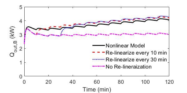
endothermically under other conditions. The search for new energy storage
technologies has led to investigation of metal hydrides for this purpose, in-
cluding using hydrides as a compact form of hydrogen storage for fuel cells
[1, 2, 3, 4, 5, 6] and for energy storage integrated with concentrated solar power
generation [7, 8, 9, 10, 11]. Systems with multiple metal hydride reactors have
also been evaluated for heating and cooling applications, where the hydride re-
actors are used in place of a heat pump [12, 13, 14, 15, 16, 17, 18]. A common
design for metal hydride systems in energy storage, heating, and cooling appli-
cations is to have a pair of metal hydride reactors connected so that hydrogen
can flow between them. In other words, as hydrogen is desorbed in one reactor,
it flows to the other reactor, which absorbs it.
   When used for energy storage, the two-reactor system does not run contin-
uously but instead absorbs heat from an external source during one half-cycle
and releases it during the other half-cycle [7, 9, 11, 19, 20]. In this application,
only one reactor is directly used for energy storage, while the other reactor is
used to store the hydrogen released by that reactor [7]. In general, two hydride
beds are not required for energy storage systems, since hydrogen released by the
metal hydride can be compressed, stored, and released from a pressure vessel
[8, 9, 10]. However, a two-reactor design is commonly studied since it allows
for more compact hydrogen storage without the need to compress hydrogen to
high pressures. The two-reactor metal hydride system is also used in single-stage
single-effect air conditioning systems, where the hydride reactions are controlled
by changing the heat sources and sinks connected to the reactors [13]. The pair
of hydride reactors undergo a two-step cycle. In the first (charging) step, the
hydride in one reactor is heated by a high-temperature heat source and desorbs
hydrogen that flows to the other reactor. Heat is released as the hydrogen is
absorbed in the second reactor, and in turn, the heat is transferred to a heat
sink at an intermediate temperature. In the second (discharging) step, the first
reactor is connected to the intermediate-temperature heat sink while the second
reactor is connected to the environment to which the cooling load needs to be
delivered. It absorbs heat from this location, providing the cooling load, as it

                                         2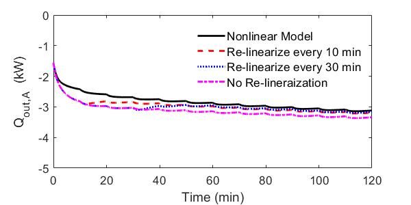
desorbs hydrogen that then flows to the other reactor [13]. In order for this
system to operate as intended, the metal hydrides have to be selected so that in
each step, changing the heat source or sink connected to the reactor results in
a temperature shift large enough to drive the desorption or absorption reaction
[16] respectively.
   If this system design is used for continuous cooling instead of energy storage,
a four-reactor system is necessary, with one reactor pair in each step of the cycle
at any given time [12, 13, 14]. An alternative design, which uses a single pair of
connected reactors, provides a continuous cooling load by using a compressor to
move hydrogen between the reactors, thus driving the reaction in each reactor
by changing the pressure, instead of the temperature [15]. This system design
requires additional power for operating the compressor, but allows for more
flexibility in choosing the specific hydrides used in the reactors. However, to
realize the benefits of this system, specifically to guarantee specific heat transfer
rates between the hydride reactors and a circulating fluid, a real-time embedded
control strategy for the system is needed.
   Numerous models of the heat and mass transfer in metal hydride reactors
have been developed. The majority of these focus on a single metal hydride
reactor, including 1-D models [21, 22] and 2-D models [23, 24, 25].            More
computationally-intensive 3-D models of a hydride reactor, first developed by
Aldas et al. [26], have been used to analyze the performance benefits of com-
plicated system geometries, such as the addition of fins [27] or a tapered bed
structure [8] to improve heat transfer. With respect to two-reactor systems,
modeling has been more limited; Kang [12] used a 1-D model to examine a
metal hydride air conditioning system and Nyamsi et al. [11] used a 3-D model
to examine a pair of hydride reactors used for energy storage. Moreover, neither
of these models considered a pair of hydride reactors with an auxiliary hydrogen
compressor.
   Similarly, control strategies for metal hydride reactors have focused on single-
reactor systems used for hydrogen storage; relevant literature is summarized in
Table 1. Since these papers are focused on a single-reactor system for hydrogen

                                         3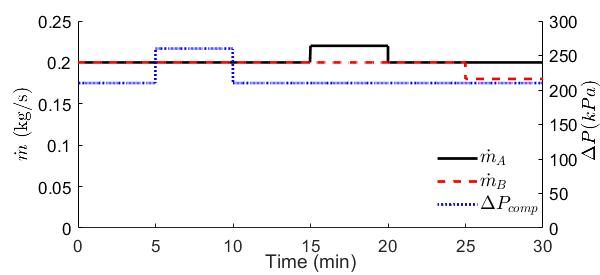
storage, the output variable of the controllers is either the hydrogen flow rate or
the temperature or pressure of the reactor, with the latter generally being used
because of its influence on the reaction rate in the reactor. For instance, while
Georgiadis et al. [6] and Panos et al. [5] use outlet temperature as the output
variable of the controller, they do so in order to achieve the outlet temperature
that will result in the optimal hydrogen release rate. Similarly, the input vari-
ables considered in all of these papers, except for Cho et al. [4], are those used
to control the heat source used to drive the desorption in the reactor, whether
that be the flow rate [6, 5] or temperature [3] of a heating fluid, or the voltage of
a thermoeletric heater [28]. While similar inputs would be considered for a case
where the hydride reactor was being used for energy storage or air conditioning,
the output variable for such cases would be the heat transfer to or from the
reactor, which is not considered by any of these controllers.
   Different models of the hydride system are also used for controller design.
For instance, Georgiadis et al. [6] use a 2-D model to determine the temperature
and pressure variations within the reactor, whereas Cho et al. [4] use a model
that neglects the effect of these variations. The linear models used for control
synthesis are obtained using model identification techniques and simulation data
from the system model [6, 5, 3]. Aruna and Jaya Christa [3] examine different
methods of converting their nonlinear model into a linear model for use in a
controller, and find the best results when using a Box-Jenkins model. All of the
methods compared are black-box methods [3]; that is, they develop the linear
model using only input and output data rather than deriving such a model from
first principles. This poses a disadvantage from the perspective of control design
because it limits the operation of the controller to a small region around the
linearization point.
   With respect to two-reactor systems, experimental demonstrations [14, 15]
used logic-based controllers to operate the system, but did not involve the design
of real-time controllers that could achieve specific heat transfer rates at specific
times, as would be desired for an energy storage system which is charged and
discharged over a longer period of time and may not be charged or discharged

                                         4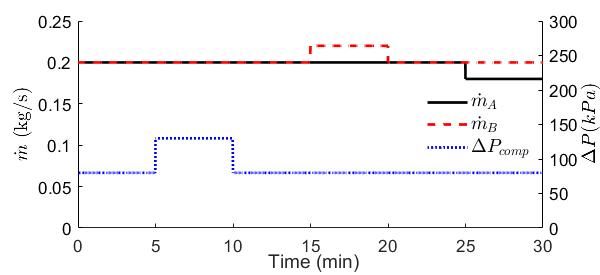
Table 1: Summary of the controller types and input and output variables that have previously
been considered for single reactor metal hydride systems.

 Author(s)             Controller                Control               Output
                                                 Variable              Variable

 Georgiadis et al.     Multi-parametric          Heating      Fluid    Outlet
 [6] 2009              (mp) MPC                  Flow Rate             Temperature
 Panos et al. [5]      mp-MPC                    Heating      Fluid    Outlet
 2010                                            Flow Rate             Temperature
 Cho et al. [4]        PID                       Discharge Valve       Hydrogen Flow
 2013                                            Opening               Rate
 Nuchkrua       and    Neuro-fuzzy PID           Thermoelectric        Reactor
 Leephakpreeda                                   Voltage               Temperature
 [28] 2013
 Aruna          and    Fuzzy PID                 Heating               Reactor
 Jaya Christa [3]                                Temperature           Pressure
 2020

continuously. These experimental systems have also used either heat transfer
from a fluid or a compressor to drive the system operation, but have not ex-
amined how to control a system that uses both. In summary, previous work
on control strategies for metal hydride reactors has not considered real-time
control for a two-reactor system using both temperature and pressure to drive
operation, nor control using a linear model derived from the system dynamics
rather than from a black-box model.
    Therefore, in this paper, we present a dynamic model for a metal hydride
energy storage system along with a model predictive control strategy for track-
ing the desired heat transfer rates in each reactor of a two-reactor metal hydride
system. Specifically, in Section 2, we present the dynamic model of the metal
hydride energy storage system including two metal hydride reactors and a com-

                                             5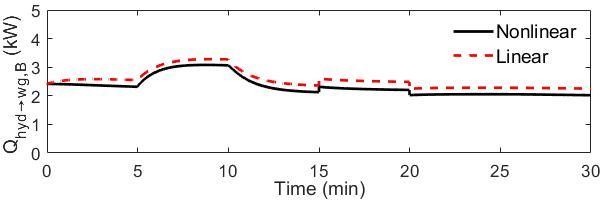
pressor to drive hydrogen flow. Then, we derive the linear state-space form of
the model using first principles. The linearized model is validated against the
nonlinear one, and we highlight how the ability to update the linearized model
enables better agreement between the linear and nonlinear models. The result-
ing model is then used for control synthesis. Because the linearized model is
physics-based and fully parameterized, it can be relinearized around any operat-
ing condition in real time, enabling it to be used beyond the nominal operating
condition. In Section 4, we present the model predictive control (MPC) design
for determining the mass flow rates of the circulating fluid and the pressure
difference between the hydrogen reactors needed to meet the demanded heat
transfer rate in each reactor. Finally, in Section 5, we demonstrate the perfor-
mance of the controller in simulation with a series of case studies. The results
indicate that the controller can achieve desired heat transfer rates between hy-
dride beds through control of the mass flow rates of the circulating fluids and
the compressor pressure. This controller enables the use of a two-reactor system
for energy storage and/or integration with a heat pump.

2. Model Description

   Here we consider a thermal energy storage system consisting of two intercon-
nected metal-hydride reactors with a compressor to drive hydrogen flow between
them, as shown in Figure 1a. Each reactor is modeled as a shell-and-tube heat
exchanger (depicted in Figure 1b) absorbing heat from, and releasing heat to,
a circulating fluid that interacts with a heat pump. We first derive a dynamic,
nonlinear thermodynamic model of the two-reactor system using first principles.
We then linearize the model to obtain a form suitable for control synthesis, and
validate the linear model against the nonlinear one.

2.1. System Model

   Each metal hydride reactor is modeled as a shell-and-tube heat exchanger.
The shell is filled with a porous bed of metal hydride through which hydrogen

                                       6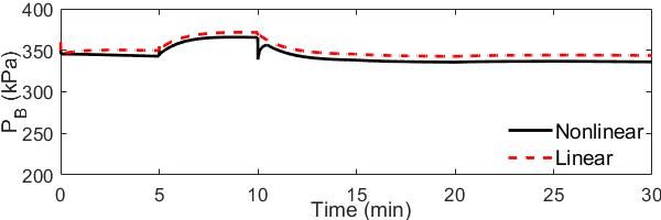
(a) Two-reactor metal hydride energy storage system

    (b) Cross-sectional view of a reactor. Seven tubes are shown for clarity, while the proposed
    system has 400 tubes within the shell.

Figure 1: Schematic of the metal hydride energy storage system. (a) Two metal hydride
reactors are connected so that hydrogen can flow between them. A compressor drives hydrogen
flow when the thermally-driven pressure gradient is unfavorable. (b) Each reactor is a shell-
and-tube heat exchanger with multiple tubes for the circulating fluid flow and a single shell
filled with metal hydride powder. To simplify the heat exchanger model, the analyzed control
volume consists of a single tube and the surrounding metal hydride as shown.

flows. Water glycol circulates in the tubes and exchanges heat with the hydride
bed. The heat exchanger is modelled using a control volume consisting of one
tube and the shell surrounding it, as shown in Figure 1b, with each other tube
and surrounding shell assumed to be the same by symmetry. The perimeter
of the heat exchanger is assumed to be insulated, so heat losses from the heat
exchanger to ambient are neglected.
    Within the control volume, it is assumed that the hydrogen in the reactors

                                                 7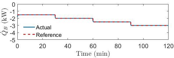
is an ideal gas, that the hydrogen and hydride in the reactor are in thermal
equilibrium (Thyd = TH ), and that all spatial variation in temperature and
pressure are negligible. Given these assumptions, the energy balance for a single
control volume is given by
                            dThyd
   (mhyd chyd + mH cp,H )         = rmhyd ∆H + ṁwg cwg (Twg,in − Thyd )
                             dt
                                              +ṁH,in cp,H (TH,in − Thyd ) ,   (1)

where mhyd and mH are the mass of the hydride and the hydrogen, respectively;
chyd , cp,H , and cwg are the specific heat of the hydride, hydrogen, and water
glycol, respectively; Thyd is the temperature of the metal hydride in the reactor,
r is the reaction rate, ∆H is the heat of reaction,  is the heat exchanger effec-
tiveness, ṁwg and ṁH,in are the mass flow rates of water glycol and hydrogen
into the reactor, and Twg,in and TH,in are the inlet temperatures of water glycol
and hydrogen, respectively. The mass balance for the hydrogen gas is given by
                             dmH
                                 = rmhyd + ṁH,in .                            (2)
                              dt
Using the ideal gas law, the pressure of the hydrogen gas, PH , can be obtained
from the mass of hydrogen as
                                       mH RH TH
                                PH =            .                              (3)
                                         VH
In this equation, RH is the gas constant for hydrogen. The volume of hydrogen
(VH ) can be found using the porosity of the metal hydride bed (φ) and the total
volume of the hydride section of the heat exchanger (Vshell ) according to

                                  VH = φVshell .                               (4)

Using Equations 3 and 4 and the thermal equilibrium assumption (Thyd =TH ),
the mass balance can be re-written in terms of pressure as
                       dPH   RThyd
                           =         (rmhyd + ṁH,in ) .                       (5)
                        dt   φVshell
   The reaction rate, r, is the rate of change of the weight fraction of hydrogen
stored in the metal hydride, w. The equations for the reaction rate and equi-
librium pressure, Peq , are taken from Voskuilen [29]. The reaction rate is given

                                        8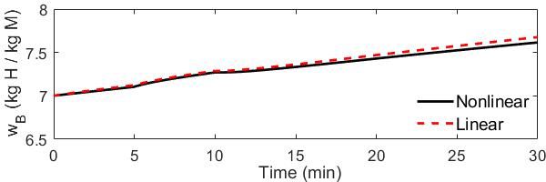
by
E
− RT A
P
C e Peq (wmax − w) ,
hyd ln P > Peq,abs
A
dw
r= = 0, Peq,des < P < Peq,abs (6)
dt EA
−
C e RThyd ln P w,
A Peq P wβ,0
In this equation, α and β are different phases of the metal hydride. The material
properties ∆H ◦ and ∆S ◦ have different values for absorption and desorption,
resulting in different equilibrium pressures for absorption and desorption.
In Equations 7 and 8, Patm is atmospheric pressure, wα,0 and wβ,0 are the
weight fractions at which the hydride phase changes, µα,0 and µβ,0 are the
chemical potential at wα,0 and wβ,0 , respectively, and Tc and A are the critical
temperature and phase interaction energy of the metal hydride, respectively.
In the energy balance, the heat exchanger effectiveness is calculated using the
expression
hA
− ṁwg cSwg
= 1−e , (9)
where h is the heat transfer coefficient and As is the surface area of the tube. The
heat transfer coefficient is calculated from the Reynolds number, ReD , Prandtl
number, P r, and thermal conductivity, k, of the fluid using the Dittus-Boelter
correlation for fully-developed turbulent flow in a circular tube [30]:
hDtube 4/5
Nu = = 0.023ReD P rn . (10)
kwg
9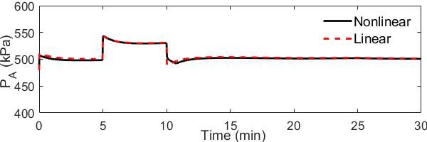
Then, the outlet temperature of the circulating fluid, Twg,out can be calculated
as
Twg,out = Twg,in + (Thyd − Twg,in ) . (11)
Thus, the heat transfer between the hydride and the water glycol, Q̇hyd→wg , is
given by
Q̇hyd→wg = ṁcwg (Twg,out − Twg,in ) = ṁcwg (Thyd − Twg,in ) . (12)
Together, Equations 1 through 12 are used to solve for the state of each reactor.
The reactors are coupled through the mass flow rate of hydrogen into the reactor,
which is calculated for one reactor as
q
Ac,Hline 2ρH (PB +∆Pcomp −PA ) , flow from B to A
Kloss
ṁH,A = q (13)
−A 2ρH (PA +∆Pcomp −PB )
c,Hline Kloss , flow from A to B
and for the other reactor as
ṁH,B = −ṁH,A . (14)
In these equations, Ac,Hline is the cross-sectional area of the hydrogen line
connecting the reactors, ρH is the density of hydrogen, ∆Pcomp is the pressure
difference created by the compressor, and Kloss is the loss coefficient for flow
from one reactor to the other. As shown in Figure 1, the compressor can drive
flow in either direction, depending on which valves are open.
2.2. Linear State-Space Model
While the governing dynamics of the two-reactor hydride system are non-
linear, the derived model is not well suited for control algorithm synthesis. An
alternative approach is to linearize the dynamics about a nominal operating
condition and synthesize a controller based on this linearized model. To that
end, we linearize the first principles model derived in the previous subsection
using a standard state-space representation as given by Equations (15) and (16)
[31].
dx
f (x, u) = = A (x − x0 ) + B (u − u0 ) + f (x0 , u0 ) (15)
dt
10g(x, u) = y = C (x − x0 ) + D (u − u0 ) + g(x0 , u0 ) (16)
Here, x is the standard state-space notation for the dynamic state vector of
the system, u is the control input vector and y is the output vector. For the case
in which one reactor, m, is absorbing hydrogen while the other, n, is desorbing,
the state, output, and input variables are defined as follows:
h iT
x= Thyd,m PH,m wm Tn PH,n whyd,n , (17)
h iT
y= Q̇hyd→wg,m Q̇hyd→wg,n , (18)
h iT
u= ṁwg,m ṁwg,n ∆Pcomp Twg,in,m Twg,in,n . (19)
Note that in these equations, the reactor where absorption occurs is always
referred to as reactor m, and the reactor where desorption occurs as reactor n,
even though these are different reactors depending on the operating mode of the
system. For brevity, the complete linearized model equations are not presented
here. However, the authors have made the linearized model code available to
the public via Github [32].
3. Linearized Model Validation
In this section, we validate the linearized model against the nonlinear one.
We first describe the specific parameterization of the model based on chosen
material properties and system dimensions, followed by a comparison of the
linearized and nonlinear models through numerical simulations.
3.1. Model Parameterization
Here we consider MmNi4.5 Cr0.5 as the material in reactor A and LaNi5 as
the material in reactor B. These materials were selected based on the operating
temperatures of an air conditioning system with which this storage system could
11ultimately be integrated. The properties of these materials are taken from the
toolbox developed by Voskuilen et al. [29] and are summarized in Table 2. By
deriving the nonlinear model, and its linearization, from first principles, the
model can easily be parameterized for any choice of metal hydrides.
Table 2: Material properties of MmNi4.5 Cr0.5 (Reactor A) and LaNi5 (Reactor B). Since the
density and specific heat of MmNi4.5 Cr0.5 are not reported in literature, they are estimated
from values for this class of alloys [29].
Property Symbol Units LaNi5 MmNi4.5 Cr0.5
Density ρ kg/m3 8300 8200
Specific Heat c J/kg·K 355 419
Enthalpy of Reaction (abs.) ∆Ha MJ/kg M 15.46 11.67
Enthalpy of Reaction (des.) ∆Hd MJ/kg M 15.95 12.65
Maximum Weight Fraction wmax kg H/kg M 0.0151 0.0121
Each hydride reactor, modeled as a shell-and-tube heat exchanger, has the
dimensions described in Table 3. The different lengths of each hydride reactor
are due to their different storage capacities and thus different volumes of hy-
dride required. The pipe for transferring hydrogen between the reactors has a
diameter of 1 cm and an assumed overall loss coefficient (Kloss ) of 40.
3.2. Simulation Results
To determine the suitability of the linear state-space model for use in con-
troller design, the dynamics predicted by the linear model are compared to those
predicted by the nonlinear model for a given set of input conditions. To compare
the models, the linear and nonlinear governing equations are simulated in MAT-
LAB using a variable-step solver that uses fifth-order numerical differentiation.
We consider two cases. In Case 1, the initial conditions are defined so that hy-
drogen is desorbed in reactor B and flows to reactor A, where it is absorbed, as
shown in Figures 3 and 4. In Case 2, the initial conditions are defined such that
12Table 3: Dimensions of the shell-and-tube heat exchangers for the hydride reactors. Only
the length varies between the two reactors. Each tube and its surrounding shell represent 1
control volume within the system shown in Figure 1.
Property Value Units
Tube Diameter 4 mm
Shell Diameter 7 mm
Number of Tubes 400 -
Length of Reactor A 1.77 m
Length of Reactor B 1.54 m
hydrogen is desorbed in reactor A and flows to reactor B where it is absorbed,
as shown in Figures 6 and 7. These two cases, with opposite reactions occur-
ring in the reactors, represent the charging and discharging modes in an energy
storage system. Note that which mode is charging and which is discharging will
depend on which reactor is being used to deliver the load. In both cases, each
of the three control input variables is perturbed for a five-minute period, and
the dynamic response of each model is observed. These perturbations to the
input variables for both cases are shown in Figure 2. For both cases, the initial
values of the state variables (x0 ), as well as the input and disturbance variables
(u0 ), are listed in Table 4, and each simulation is initialized at the linearization
point (x0 , u0 ).
(a) Case 1 (b) Case 2
Figure 2: Input circulating fluid mass flow rate and compressor pressure difference for (a)
Case 1 and (b) Case 2.
13Table 4: Initial values for the state and input variables. Note that kg H indicates mass of
hydrogen and kg M indicates mass of the metal hydride.
Variable Case 1 Case 2 Units
◦
Thyd,A 6.89 6.89 C
◦
Thyd,B 36.9 34.9 C
PH,A 480 290 kPa
PH,B 290 360 kPa
wA 0.006 0.007 kg H / kg M
wB 0.006 0.007 kg H / kg M
ṁwg,A 0.2 0.2 kg/s
ṁwg,B 0.2 0.2 kg/s
∆Pcomp 210 80 kPa
◦
Twg,in,A 1.89 11.9 C
◦
Twg,in,B 42.9 30.9 C
In both cases, the linear model matches the nonlinear model closely. This is
quantified using the root mean square error (RMSE) between the state variables
predicted by the linear model and the nonlinear model, as shown in Table 5.
The normalized RMSE (NRMSE) values were calculated using Equation 20. All
variables of the same type (e.g. temperature, pressure, or weight fraction) were
normalized against the same value, determined by finding the maximum range
over which each variable varies in either reactor (A or B) in either of the two
simulation cases (see Equations 21- 22, where the subscript i refers to the initial
value of a given state variable simulated for a given case study).
RM SE
N M RSE = (20)
max(∆xA , ∆xB )
14(a) Hydride Temperature in Reactor A (b) Hydride Temperature in Reactor B
(c) Hydrogen Pressure in Reactor A (d) Hydrogen Pressure in Reactor B
(e) Hydrogen Weight Fraction in Reactor A (f) Hydrogen Weight Fraction in Reactor B
Figure 3: Comparison of the dynamic state variables for Reactors A and B between the linear
model (dashed lines) and the nonlinear model (solid lines) for Case 1 (hydrogen flowing from
reactor A to reactor B).
(a) Reactor A (b) Reactor B
Figure 4: Comparison of the heat transfer rates associated with Reactors A and B between
the linear model (dashed lines) and the nonlinear model (solid lines) for Case 1 (hydrogen
flowing from reactor A to reactor B).
∆xA = max (max(xA − xA,i )Case1 , max(xA − xA,i )Case2 ) −
min (min(xA − xA,i )Case1 , min(xA − xA,i )Case2 ) (21)
15∆xB = max (max(xB − xB,i )Case1 , max(xB − xB,i )Case2 ) −
min (min(xB − xB,i )Case1 , min(xB − xB,i )Case2 ) (22)
Table 5: RMSE and NRMSE for all state variables for Case 1.
RMSE
gH gH
t(min) Thyd,A (◦ C) Thyd,B (◦ C) PH,A (kPa) PH,B (kPa) wA ( kg M) wB ( kg M)
0−5 0.095 0.248 3.08 3.70 0.0047 0.0074
5 − 10 0.156 0.384 0.477 6.06 0.0060 0.017
10 − 15 0.094 0.354 2.66 7.23 0.0034 0.022
15 − 20 0.077 0.376 2.66 7.23 0.0061 0.029
20 − 25 0.057 0.388 0.847 6.70 0.0082 0.036
25 − 30 0.041 0.389 0.622 7.04 0.010 0.042
NRMSE
t(min) Thyd,A Thyd,B PH,A PH,B wA wB
0−5 2.42% 6.29% 2.26% 2.72% 0.356% 0.561%
5 − 10 3.96% 9.75% 0.349% 4.44% 0.455% 1.26%
10 − 15 2.37% 8.97% 1.95% 5.30% 0.258% 1.68%
15 − 20 1.94% 9.55% 0.918% 4.58% 0.462% 2.20%
20 − 25 1.45% 9.84% 0.621% 4.92% 0.621% 2.69%
25 − 30 1.05% 9.88% 0.456% 5.16% 0.780% 3.19%
For Case 1, the fastest response in the system is that of the hydrogen pressure
(seen in Figures 3c and 3d) to the change in the pressure difference created by the
compressor (∆Pcomp ) at t = 5 min and at t = 10 min. At t = 5 min, increasing
∆Pcomp results in an almost immediate change in the hydrogen pressure of
reactor A (PH,A ) approximately equal to the change in ∆Pcomp , as seen in
Figure 3c. To understand why PH,A changes more than PH,B , we can revisit
the two terms of the pressure balance given in Equation 5 (repeated below for
convenience): the absorption or desorption rate (depending on the direction of
16the reaction) rmhyd , and the hydrogen mass flow rate into the reactor, ṁH,in .
dPH RThyd
= (rmhyd + ṁH,in )
dt φVshell
At this operating condition, rB (the reaction rate on a per unit mass of hydride
basis) is more sensitive to changes in pressure than rA . When ∆Pcomp increases,
the magnitude of ṁH,in increases in each reactor. This term becomes much
larger than the absorption rate in reactor A or the desorption rate in reactor
B. However, the desorption rate in reactor B increases enough to balance the
mass flow rate after only a small change in PH,B , while it takes a much larger
change in PH,A before the absorption rate in reactor A balances the mass flow
rate. Thus, PH,A increases much more than PH,B decreases. This process occurs
very quickly; in the initial second after ∆Pcomp increases, the driving pressure
difference PH,B + ∆Pcomp − PH,A decreases by 94.8%. Thus, it appears as a
step change when plotted over a 30-minute time span in Figure 3c. The linear
state-space model successfully captures this response, as seen in Figures 3c and
3d.
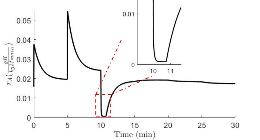
At t = 10 min, when ∆Pcomp returns to its original value, there is a signif-
icant step change in both pressures. The change in ∆Pcomp causes hydrogen
to flow from reactor A to reactor B, whereas it otherwise flows from reactor
B to reactor A in Case 1. Therefore, in both reactors, rmhyd and ṁH,in have
the same sign, so rB mhyd,B cannot balance ṁH,in,B as it did before. Once
the initial pressure difference has been reduced, the mass flow is reduced to a
small value, so the changes in pressure are primarily due to the reaction rates.
However, the response of rB to the change in the pressure causes rB to go to
zero, as shown in Figure 5b. As shown in Figure 5a, however, rA decreases but
does not go to zero. This means that for approximately 45 seconds, hydrogen is
being absorbed in one reactor but not desorbed in the other. Thus, the pressure
in both reactors slowly decreases, since hydrogen is flowing out of reactor B,
but the absorption rate in reactor A is larger than the flow rate in. After ∼45
seconds, the increasing temperature seen in Figure 3b causes the absorption
rate for reactor B to grow larger than ṁH,in,B , so PH,B starts increasing. This
17increase leads to an increased mass flow rate to reactor A, which is larger than
the absorption rate in reactor A, resulting in PH,A increasing as well.
(a) Reactor A (b) Reactor B
Figure 5: Reaction rates in Reactors A and B for Case 1 (hydrogen flowing from reactor A to
reactor B).
The most significant difference between the linear and nonlinear models can
be seen in Figure 3d, where the linear model does not capture the initial spike in
PH,B and the decay that follows it, but accurately captures the behavior of the
pressure after that time. This is because the reaction rate equation (Equation 6)
is discontinuous when it goes to zero; as shown in Equation 6. Since the linear
model does not include this discontinuity, it fails to capture the behavior of the
pressure while the reaction rate is equal to zero. However, once the reaction
rate is again nonzero, the linear model again follows the nonlinear model.
The response of the hydride temperature in each reactor to the change in
∆Pcomp is shown in Figures 3a and 3b. Here, the increased reaction rate after
the increase in ∆Pcomp results in an increase in the heat released or absorbed
by the reaction, pushing the temperature of the hydrides in both reactors away
from the temperature of the circulating fluid in their reactors. This causes
the heat transfer rate between the hydride in each reactor and the circulating
fluid to increase, as shown in Figure 4. Once these heat transfer rates are
approximately equal to the heat transfer from absorption and desorption, the
temperatures become close to steady. While the linear model underestimates
Thyd,B after the step change, as shown in Figure 3b at t = 5 min, it stays
within 10% of the nonlinear model, and Thyd,A stays within 5% throughout the
18simulation.
In contrast to the visible changes in pressure and temperature that occur
when ∆Pcomp changes, there is not a significant change in these variables when
either of the mass flow rates are changed. However, as shown in Figure 4, there
is a step change in the heat transfer rate in each reactor when there is a change
in the mass flow rate in that reactor. This is because the heat transfer rate is
a linear function of the mass flow rate. This change is accurately captured by
the linear model, as seen in Figures 4a and 4b. All variables stay within 10% of
the nonlinear model throughout the simulation.
Finally, the change in the weight fraction over time is different from that
of the hydride temperature and pressure because the weight fraction changes
continually (except for wB while rB is equal to zero) and does not enter a near-
equilibrium state. The dynamics of the weight fraction are controlled by the
reaction rate, which is the derivative of the weight fraction. As discussed in
regards to the pressure dynamics, the reaction rate in both reactors changes
quickly in the seconds after the change in ∆Pcomp until rA mhyd,A , rB mhyd,B ,
and ṁH,in have approximately equal magnitudes. This quick change in the
reaction rate, combined with the very slow change for the rest of the simulation
period, results in the weight fraction in each reactor resembling a linear function
with a different slope after t = 5 min, as seen in Figures 3e and 3f. After
∆Pcomp returns to its original value at t = 10 min, the rate of change of the
weight fraction also returns to approximately its original value. For the weight
fraction, the error of the linear models stays below 4% for both reactors as shown
in Table 5. Like the pressure, the weight fraction does not respond significantly
to changes in the mass flow rates.
For Case 2, despite hydrogen flow in the system moving in the opposite
direction, the same trends can be seen as discussed for Case 1. The pressure
dynamics are similar, including rB going to zero for some time after t = 10 min.
However, because reactor A is desorbing hydrogen here rather than absorbing
it as in Case 1, the pressure in both reactors increases while rB equals zero, and
then decreases once absorption starts in reactor B, as seen in Figures 6c and 6d.
19(a) Hydride Temperature in Reactor A (b) Hydride Temperature in Reactor B
(c) Hydrogen Pressure in Reactor A (d) Hydrogen Pressure in Reactor B
(e) Hydrogen Weight Fraction in Reactor A (f) Hydrogen Weight Fraction in Reactor B
Figure 6: Comparison of the state variables for Reactors A and B comparing the linear model
(dashed lines) to the nonlinear model (solid lines) for Case 2 (hydrogen flowing from reactor
B to reactor A).
(a) Reactor A (b) Reactor B
Figure 7: Comparison of the heat transfer rates out of Reactors A and B comparing the linear
model (dashed lines) to the nonlinear model (solid lines) for Case 2 (hydrogen flowing from
reactor B to reactor A).
The same general trends can also be seen in the temperature and weight fraction
dynamics, with the only differences being due to the reversal of which reactor
is absorbing hydrogen and releasing heat to the circulating fluid, and which is
desorbing hydrogen and being heated by the circulating fluid.
Overall, the linear model predictions match those of the nonlinear model well
20Table 6: RMSE and NRMSE for all state variables for Case 2.
RMSE
◦ ◦ gH gH
t(min) Thyd,A ( C) Thyd,B ( C) PH,A (kPa) PH,B (kPa) wA ( kg M) wB ( kg M)
0−5 0.273 0.380 1.01 5.22 0.011 0.012
5 − 10 0.317 0.400 0.829 5.55 0.017 0.017
10 − 15 0.391 0.455 1.16 7.46 0.025 0.023
15 − 20 0.428 0.474 0.787 7.01 0.033 0.034
20 − 25 0.424 0.476 0.980 7.29 0.039 0.045
25 − 30 0.407 0.479 1.17 7.58 0.045 0.056
NRMSE
t(min) Thyd,A Thyd,B PH,A PH,B wA wB
0−5 6.92% 9.66% 0.743% 3.83% 0.811% 0.886%
5 − 10 8.05% 10.2% 0.608% 4.07% 1.30% 1.27%
10 − 15 9.93% 11.6% 0.851% 5.47% 1.89% 1.75%
15 − 20 10.9% 12.0% 0.577% 5.14% 2.46% 2.61%
20 − 25 10.8% 12.1% 0.718% 5.34% 2.95% 3.43%
25 − 30 10.3% 12.1% 0.858% 5.55% 3.42% 4.23%
in Case 2. As seen in Table 6, there is a larger error for the hydride temperature
states in this case than for Case 1, but the linear model is still accurate within
12.5% across the entire simulation period. The error for PH,A is lower for this
case, remaining within 1% of the nonlinear model, while the highest error for
PH,B is still less than 6% different from the nonlinear model. The error between
the linear and nonlinear model predictions for the weight fraction states follows a
similar pattern to Case 1, continually increasing over time while never exceeding
5%, without any of the changes to the inputs noticeably affecting the rate at
which the error increases.
213.3. Resetting the Linearization Point
While the validation results show that the linear model predicts the system
dynamics accurately within approximately 12.5% of the linearization point, it
is expected that during operation, the system will deviate further from a single
point. This can adversely affect the controller design if it assumes the dynamics
do not vary from a single linear model. One way to address this is to periodically
re-linearize the model around the current operating condition. To illustrate
how re-linearization affects the accuracy of the linear model, we simulate both
the nonlinear and linear models for 120 minutes, beginning with the initial
conditions shown in Table 7. In order to sustain the absorption and desorption
reactions in the reactors for 120 minutes, the compressor pressure difference is
increased by 10 kPa every 10 minutes. We compare three different cases: 1)
simulating the linear model from the same initial conditions without any re-
linearization, 2) simulating the linear model beginning with the same initial
conditions but then re-linearizing it every 10 minutes, and 3) simulating the
linear model beginning with the same initial conditions but then re-linearizing it
every 30 minutes. The resulting heat transfer rates for these cases are compared
against the nonlinear model simulation in Figure 8, and the RMSE for the heat
transfer rates is given in Table 8. It is worth noting that because the linearized
model is fully parameterized, re-linearizing is equivalent to updating the model
parameters. In other words, re-linearizing does not contribute any significant
computational complexity to the numerical simulation.
From Figure 8 we can see that re-linearization does improve the accuracy
of the linear model over the duration of the simulation. For both heat trans-
fer rates, both cases with re-linearization match the nonlinear model after re-
linearization more closely than the case without re-linearization. It is worth
noting that the extent of the nonlinearity of each reactor is not the same. For
reactor A, as shown in Figure 8a, even without re-linearization, the linear model
matches the nonlinear one on average within 0.35 kW. Furthermore, the linear
model does not diverge from the nonlinear model: the error for the last 30 min-
utes is less than that for the first 30 minutes. For reactor B, as shown in Figure
22Table 7: Initial values for the state and input variables for comparing performance with and
without re-linearizing the model and for the case in which the controller is used for flow from
reactor B to reactor A.
Variable Value Units Variable Value Units
◦
Ti,A 6.9 C ṁwg,A 0.2 kg/s
◦
Ti,B 34. C ṁwg,B 0.2 kg/s
Pi,A 290 kPa ∆Pcomp 80 kPa
◦
Pi,B 360 kPa Twg,in,A 12 C
◦
wi,A 0.008 kg H / kg M Twg,in,B 27 C
wi,B 0.0045 kg H / kg M
(a) Reactor A (b) Reactor B
Figure 8: Heat transfer rates from the hydride beds to the circulating fluid in each reactor.
The performance of the linear models is compared to the nonlinear model (solid black line) for
three different cases: one where the model is never re-linearized (dot-dashed pink line), one
where it is re-linearized every 10 minutes (dotted blue line), and one where it is re-linearized
every 30 minutes (dashed red line). Throughout this study, the compressor pressure difference
is increased by 10 kPa every 10 minutes.
8b, the model with no re-linearization diverges from the nonlinear model almost
immediately, with error increasing over time.
Comparing the performance of the linear model with re-linearization every 10
minutes to that with re-linearization every 30 minutes, we can see in Table 8 that
both stay within 0.2 kW of the nonlinear model after the first 30 minutes. The
difference in error between them is small, with more frequent re-linearization
23Table 8: RMSE for the heat rates for the 3 cases studied. All values are in kW.
No Relin. Every 10 min Every 30 min
t(min) QA QB QA QB QA QB
0 − 30 0.338 0.376 0.251 0.154 0.338 0.376
30 − 60 0.308 0.596 0.127 0.179 0.186 0.148
60 − 90 0.257 0.796 0.101 0.166 0.081 0.196
90 − 120 0.228 0.983 0.081 0.145 0.061 0.182
never resulting in a reduction in error of more than 0.03 kW once both models
have been re-linearized at least once. In general, the frequency with which the
parameters of the linear model should be updated will depend on how close the
last linearization point is to the “near-equilibrium” state in which there is only a
slow change in the temperature, pressure, and reaction rate in each reactor. For
the operating conditions considered here, we can conclude that re-linearizing
every 30 minutes is sufficient for maintaining accuracy; this will be applied to
the controller design discussed in the next section.
4. Controller Design and Synthesis
In this section, we describe the design of a multi-input-multi-output (MIMO)
model predictive controller (MPC) for regulating the operation of the proposed
two-reactor metal hydride thermal energy storage system.
4.1. Model Predictive Control Algorithm
MPC is a control technique that utilizes a model of the system dynamics to
optimize a sequence of control inputs over a specified time horizon by predict-
ing the dynamical response of the system over said horizon based on different
sequences of inputs [33]. At each measurement sample, MPC involves solving
an N -step ahead online optimization problem to predict the optimal sequence
24of control inputs [u (k) , u (k + 1) , · · · u(k + N )] that will drive the output se-
quence [y (k) , y (k + 1) , · · · y(k + N )] toward a desired reference trajectory. At
each time in the control sampling period, the MPC problem is solved, and the
optimized variables u (k) are taken as the control input at that sample instant.
Given the nonlinear dynamics of the hydride system, a successive lineariza-
tion technique [34] is used with a linear MPC design to achieve the desired con-
trol objectives. As was shown in Sec. 3, local linearization of the model matches
the nonlinear model within 12.1% (based upon the validation presented in Sec-
tion 3) and is therefore adequate for use as a prediction model in a MPC design.
We design and implement the MPC as a discrete-time controller. Therefore, the
state dynamics and system outputs are discretized and expressed as
x (k + 1) = Ax (k) + Bu (k) + Bd d(k) (23)
y (k) = Cx (k) + Du (k) + Dd d(k) .
In these equations, the input vector has been separated into u and d, where
u is the set of input variables we can control (mass flow rates and compres-
sor pressure difference), while d is the set of disturbance inputs (circulating
fluid inlet temperatures), i.e. those input variables that cannot be controlled
. To achieve zero steady-state tracking error, we augment the linear-quadratic
regulator (LQR) with integral control as shown in Equation (24):
˜
x̃ (k + 1) = Ãx̃ (k) + B̃u (k) + B̃d d(k) (24)
ỹ (k) = C̃x̃(k) ,
where
A 0 B B 0 h i
à = , B̃ = , B̃d = d , C̃ = 0 I , (25)
C 0 D Dd −I
h iT h iT
and x̃ (k) = x (k) , xi (k) ˜
and d(k) = d (k) r (k) . Based on Equa-
tion (25), the output of the control model simplifies to ỹ (k) = xi (k) where
25xi (k + 1) = Q̇ (k) − r(k). Therefore, the MPC is formulated as an error reg-
ulation problem to drive xi (k) to zero, which is equivalent to driving the heat
transfer rates Q̇ (k) to the reference values r(k). The MPC problem can be
stated as
N
X T T
min J = ye (k) Qe
y (k) + u (k) Ru (k)
U,Y
k=1
s.t. x
e (k + 1) = Ae
e x (k) + Bu e d de(k) ∀ k ∈ [1, N ]
e (k) + B
(26)
e x (k + 1) ∀ k ∈ [1, N ]
ye (k + 1) = Ce
umin ≤ u (k) ≤ umax ∀ k ∈ [1, N ]
|u (k) − u (k + 1) | ≤ δumax ∀ k ∈ [1, N − 1] ,
where
U = [u (k = 1) , u (2) , . . . , u (N )]
Y = [e
y (k = 1) , ye (2) , . . . , ye (N )] ,
and Q and R are positive definite weighting matrices. The constraints ensure
(1) adherence to the state dynamics prescribed by the control model given in
Equations (24) and (25), (2) that the optimal values for the inputs u are within
the achievable range of inputs, and (3) that the rate of change in the chosen
inputs does not exceed actuator limits.
4.2. Controller Synthesis
For the simulated case studies, the results of which are presented in Sec-
tion 5, the matrices Q and R are tuned to penalize tracking error and the
magnitude of the control inputs, respectively. The relative magnitude of the
weights in these matrices drives the controller performance, and can be moti-
vated by the dynamics of the system itself. One representative linearization of
the model, corresponding to Case 1 as described later in Section 5, is shown in
Equations (29) - (34).
26In the two-reactor hydride system, the output variables Q̇hyd→wg,m and
Q̇hyd→wg,n are directly affected by the mass flow rate of the circulating fluid in
each reactor, ṁwg,m and ṁwg,n , respectively, through the D matrix. Note that
these correspond to the first two inputs defined in the input vector u. The third
input variable, the compressor pressure difference ∆Pcomp , does not directly
affect the output variables; it only indirectly affects them through its effect
on the hydride temperature states, Thyd,m and Thyd,n . Therefore, in tuning
Q and R, we more heavily penalize ∆Pcomp , relative to the weights placed on
ṁwg,m and ṁwg,n , to incentivize the controller to use ∆Pcomp to help regulate
Q̇hyd→wg,m and Q̇hyd→wg,n . The final weights chosen for Q and R are
100 0
Q= (27)
0 100
3 × 10¹¹ 0 0
R= 3 × 10¹¹ 0 . (28)
0
0 0 1
We formulate and solve the MPC as a quadratic program using the quad-
prog solver within the MATLAB Optimization Toolbox [35]. Formulating the
problem as a quadratic program permits a computationally-efficient controller
synthesis to be obtained for each control sample with little computational over-
head.
Thyd,m Thyd,m
ṁwg,m
PH,m PH,m
ṁwg,n
d wm wm
f (x, u) = = A + B ∆P (29)
comp
dt
Thyd,n
Thyd,n
T wg,in,m
PH,n PH,n
Twg,in,n
whyd,n whyd,n
27
−8.17 × 10⁻³ −3.35 × 10⁻⁸ −8.13 −9.07 × 10⁻⁵ 4.09 × 10⁻⁷ 0
−4.38 1.11 × 10⁷
8840 0 3.96 0
−2.28 × 10⁻⁷ 1.38 × 10⁻¹¹ −2.93 × 10⁻⁴
0 0 0
(30)
A=
−0.216 1.83 × 10⁻⁵ −94.4
0 0 0
2.03 × 10⁵ −22.4 9.00 × 10⁷
0 4.93 0
0 0 0 −4.78 × 10⁻⁶ 4.09 × 10⁻¹⁰ −2.12 × 10⁻³
−0.039 0 4.47 × 10⁻⁷ 1.68 × 10⁻³ 0
0 0 3.91 0 0
0 0 0 0 0
B= (31)
−3
2.99 × 10
0 0.064 0 0
−5.00
0 0 0 0
0 0 0 0 0
Thyd,m
ṁ wg,m
PH,m
ṁ wg,n
Q̇hyd→wg,m w
g(x, u) = = C m + D ∆P comp
(32)
Q̇hyd→wg,n Thyd,n
T wg,in,m
PH,n
Twg,in,n
whyd,n
367.1 0 0 0 0 0
C= (33)
0 0 0 436.3 0 0
7930 0 0 −341 0
D= (34)
0 −9600 0 0 −452
5. Results
In this section, we implement the controller in simulation and demonstrate
its performance in regulating the dynamics of the two-reactor metal hydride
system through a series of case studies.
285.1. Reference Tracking
The MPC is designed primarily for referencing tracking, so we first verify
its performance in the context of tracking variable heat transfer rates in each
reactor. The model is simulated using the same initial conditions as those given
in Table 4. Moreover, the control input variables are bounded based on the
values shown in Table 9.
Table 9: Upper and lower bounds on the control input variables.
Variable Units Minimum Maximum
ṁA kg/s 0 0.8
ṁB kg/s 0 0.8
∆Pcomp kPa 0 500
The model is simulated for a two-hour period with the desired heat transfer
rate setpoints (reference values) changing every 30 minutes and the controller re-
linearizing around the current operating point when the setpoint changes. The
control input variables are updated at a frequency of 1 Hz. As with the model
validation, two cases are considered, representing the two operating modes of
the system. In Case 1, the reference value for the heat transfer rate in Reactor A
increases over a series of three step changes which are mirrored by step decreases
in the heat transfer rate in Reactor B. The opposite trends in the references are
demonstrated in Case 2. The closed-loop simulation results for Case 1 are shown
in Figure 9. The results for Case 2 are given in Appendix A.
Figure 9 shows that the controller successfully tracks the step changes in
the heat transfer rates in each reactor, doing so primarily through adjustments
in each of the circulating fluid mass flow rates (see Figures 9a and 9c). This
is consistent with the algebraic relationship between mass flow rate and heat
transfer rate in each reactor. In addition, the mass flow rates slowly increase
over time in between step changes, adjusting to maintain a fixed heat transfer
29(a) Circulating Fluid Mass Flow Rate A (b) Heat Transfer Rate in Reactor A
(c) Circulating Fluid Mass Flow Rate B (d) Heat Transfer Rate in Reactor B
(e) Compressor Pressure Difference
Figure 9: Input values set by the controller and output heat transfer rates in the hydride
reactors compared to the reference value for the case where hydrogen is being moved from
reactor B to reactor A. The model is re-linearized and the reference value changed every 30
minutes.
rate while the temperature differential between each reactor and the associated
circulating fluid decreases. As shown in Figure 9e, the controller makes less
use of the compressor pressure difference to achieve its objectives. While its
value does change over time, the difference between the minimum and maximum
values of ∆Pcomp is only around 1% of the range of values the controller can set
it to, while the difference between the minimum and maximum values of ṁA is
approximately 50% of its range.
For both this case and the case given in Appendix A, the ratio of the heat
transfer rates in the two reactors are held constant even when the magnitude of
the reference (desired) heat transfer rate changes. Specifically, the heat transfer
rate in reactor A has the opposite sign and 85% of the magnitude of that in
reactor B. To see how the controller performance changes for a different ratio
30between the heat transfer rates, we consider a case with the same initial con-
ditions and reference values for Q̇B as defined in Case 1, but with the ratio of
the magnitudes of the heat transfer rates set to 1. The control input signals
and resulting heat transfer rates, compared to the reference values, are shown
in Figure 10.
(a) Circulating Fluid Mass Flow Rate A (b) Heat Transfer Rate in Reactor A
(c) Circulating Fluid Mass Flow Rate B (d) Heat Transfer Rate in Reactor B
(e) Compressor Pressure Difference
Figure 10: Input values set by the controller and output heat transfer rates in the hydride
reactors compared to the reference value for the case where hydrogen is being moved from
reactor B to reactor A and the ratio between heat transfer rates is set to 1 instead of 0.85.
The model is re-linearized and the reference value changed every 30 minutes.
A major departure in these results, as compared to those shown in Case
1, is the response of the controller when the circulating fluid mass flow rate
through reactor A saturates at its upper bound of 0.8 kg/s as shown at t = 80
min in Figure 10a. The MPC, recognizing this constraint, begins to increase
the pressure differential across the compressor, since this is now the best input
variable to use to control the heat transfer rate in Reactor A (see Figure 10e).
Figure 10b shows that the compressor is able to track the reference using the
31compressor pressure difference, but that the system is slower to respond given
that the compressor pressure difference has a dynamic, rather than algebraic,
effect on the output. While Reactor A requires a larger mass flow rate over
time because the reactor temperature is approaching the circulating fluid tem-
perature, in Reactor B, the reactor temperature diverges from the circulating
fluid temperature. Thus, as shown in Figure 10c, the mass flow rate required to
meet the reference heat transfer rate decreases over time, so much so that that
the input mass flow rate values used to achieve the final reference heat transfer
rate are similar to the values used to achieve the initial value, albeit the final
reference value is much larger.
Given the coupling of the dynamics between the two reactors, it is desirable
to operate the system in a near-equilibrium state. This avoids the situation
in which the compressor pressure difference and the mass flow rate in one re-
actor are saturated, which would degrade the performance of the controller.
Near equilibrium, the absorption or desorption rate in each reactor balances
the mass flow rate between them, and the energy transfer from the reaction
balances the heat transfer to the circulating fluid in each reactor. It is therefore
important to select a ratio between the reference heat transfer rates that allows
for near-equilibrium operation if the controller is being used for a full charging
or discharging cycle.
5.2. Disturbance Rejection
To test the controller’s ability to mitigate exogenous disturbances, we con-
sider constant heat transfer rate references in each reactor for the same sets of
initial conditions described in the previous section, but now change the circulat-
ing fluid temperatures every 10 minutes as shown in Figure 11f. For this case,
the model is still re-linearized every 30 minutes. The control input signals and
resulting heat transfer rates are compared to their reference values in Figure 11.
As shown in Figure 11, the controller quickly adjusts to the changes in the
disturbance inputs, successfully minimizing regulation error after only a very
brief deviation away from the desired heat transfer rate. The first of these
32(a) Circulating Fluid Mass Flow Rate A (b) Heat Transfer Rate in Reactor A
(c) Circulating Fluid Mass Flow Rate B (d) Heat Transfer Rate in Reactor B
(e) Compressor Pressure Difference (f) Circulating Fluid Temperatures
Figure 11: Input values set by the controller and output heat transfer rates in the hydride
reactors for the case where hydrogen is being moved from reactor B to reactor A, compared
to their reference values. The circulating fluid temperature changes every 10 minutes and the
model is re-linearized every 30 minutes.
spikes can be seen in more detail in Figure 12, which shows the 1-minute period
of time around the change in the disturbance inputs. From this, we can see
that the controller converges to the reference value within 5-6 seconds. As with
the case in which we considered time-varying heat transfer rates, the controller
primarily changes the mass flow rates in order to track the reference, but does
make some small changes to the compressor pressure difference. The controller
is robust to changes in the disturbance inputs despite using a prediction model
that is re-linearized less frequently than the disturbance signals change.
In a further test of the ability of the controller to mitigate changes in the
disturbance inputs, the controller was simulated for the initial conditions given
in Case 2, with a larger change in the water glycol temperatures. Results for
this case are given in Appendix B.
33(a) Heat Transfer Rate A (b) Heat Transfer Rate B
Figure 12: Heat transfer rates in the reactors for Case 1 from 9.5 to 10.5 minutes.
6. Conclusion
In this paper we presented a a model predictive controller (MPC) for a
two-reactor metal hydride system in which reactions in each hydride bed are
driven by heat transfer between the metal hydride and a circulating fluid as
well as a compressor moving hydrogen between the reactors. The multivariable
controller successfully tracks desired values for the heat transfer between the
hydride bed and the circulating fluid in each reactor by controlling the pressure
difference produced by the compressor and the mass flow rates of the circulat-
ing fluid in each reactor. We derived a first-principles nonlinear dynamic model
of the two-reactor system, and then linearized it for the purposes of control
design. While the nonlinear model of the reactor neglects any temperature or
pressure gradients within the hydride beds, it predicts the evolution of the re-
actor pressure, temperature, and heat transfer rates to the circulating fluid. By
analytically linearizing the nonlinear model, we obtained a parameterized state-
space model that could be easily updated for different operating conditions.
This was leveraged in the design of the MPC, in which the linear prediction
model was periodically re-linearized to minimize differences between its predic-
tions and the dynamics of the nonlinear model. Through a series of simulated
case studies, we demonstrated the performance of the controller for both refer-
ence tracking and disturbance rejection. The proposed model and multivariable
controller enable continuous operation of two-reactor metal hydride systems to
regulate heat transfer in a metal hydride energy storage or A/C system. Areas
of future research include examining the viability of controlling heat transfer in
one reactor while minimizing temperature change in both, as well as testing the
34controller for use with higher-order models and real hydride systems.
Acknowledgements
Funding for this project was provided by the Center for High-Performance
Buildings at Purdue University.
Model Availability
The code used to linearize the nonlinear dynamics model is available as Mat-
lab .m files on Github at https://github.com/patrickkrane/hydride-linearization-
model.git.
References
[1] M. Tange, T. Maeda, A. Nakano, H. Ito, Y. Kawakami, M. Masuda,
T. Takahashi, Experimental study of hydrogen storage with reaction heat
recovery using metal hydride in a totalized hydrogen energy utilization sys-
tem, International Journal of Hydrogen Energy 36 (2011) 11767–11776.
[2] A. Khayrullina, D. Blinov, V. Borzenko, Air heated metal hydride energy
storage system design and experiments for microgrid applications, Inter-
national Journal of Hydrogen Energy (2018) 1–9.
[3] R. Aruna, S. T. Jaya Christa, Modeling, system identification and design
of fuzzy PID controller for discharge dynamics of metal hydride hydrogen
storage bed, International Journal of Hydrogen Energy 45 (2020) 4703–
4719.
[4] J. H. Cho, S. S. Yu, M. Y. Kim, S. G. Kang, Y. D. Lee, K. Y. Ahn, H. J.
Ji, Dynamic modeling and simulation of hydrogen supply capacity from a
metal hydride tank, International Journal of Hydrogen Energy 38 (2013)
8813–8828.
35You can also read