A Total Lagrangian SPH Method for Modelling Damage and Failure in Solids
←
→
Page content transcription
If your browser does not render page correctly, please read the page content below
A Total Lagrangian SPH Method for Modelling Damage and
                                                                     Failure in Solids
                                                                               Md Rushdie Ibne Islama , Chong Penga,b,∗
                                                                 a
                                                                     ESS Engineering Software Steyr GmbH, Berggasse 35, 4400 Steyr, Austria
                                                    b
                                                        Institut für Geotechnik, Universität für Bodenkultur, Feistmantelstrasse 4, 1180 Vienna, Austria
arXiv:1901.08342v1 [cs.CE] 24 Jan 2019

                                         Abstract
                                         An algorithm is proposed to model crack initiation and propagation within the total Lagrangian
                                         Smoothed Particle Hydrodynamics (TLSPH) framework. TLSPH avoids the two main deficiencies
                                         of conventional SPH, i.e., tensile instability and inconsistency, by making use of the Lagrangian
                                         kernel and gradient correction, respectively. In the present approach, the support domain of a
                                         particle is modified, where it only interacts with its immediately neighbouring particles. A virtual
                                         link defines the level of interaction between each particle pair. The state of the virtual link is
                                         determined by damage law or cracking criterion. The virtual link approach allows easy and natural
                                         modelling of cracking surfaces without explicit cracking treatments such as particle splitting, field
                                         enrichment or visibility criterion. The performance of the proposed approach is demonstrated via
                                         a few numerical examples of both brittle and ductile failure under impact loading.
                                         Keywords: TLSPH, Fracture model, Crack growth, Brittle and Ductile damage, Dynamic loading

                                         1. Introduction
                                             Initiation and propagation cracks, propagation and their interaction are often encountered in
                                         solid mechanics problems. Materials under different loading conditions may undergo various
                                         stages before complete failure. Therefore, one of the primary aims of computational mechan-
                                         ics is to simulate the cracks and their propagation accurately. Earlier attempts are mostly based on
                                         grid/mesh-based methods such as the Finite Element Method (FEM). Despite being popular and
                                         successful methods for modelling of solids, FEM and other grid-based methods suffer from sig-
                                         nificant drawbacks in modelling discrete cracks due to the presence of grids or meshes [1]. Many
                                         attempts are made to model the cracks and their propagation through special treatments such as
                                         mesh refinement and field enrichments etc. [2, 3, 4, 5]. However, it is still quite challenging to
                                         model multiple crack paths, their propagation and interaction. Furthermore, if the material un-
                                         dergoes finite deformation, the grid/mesh suffers from mesh entanglement, mesh distortion etc.,
                                         which affect the accuracy of the solution significantly. Moreover, the grid-based methods require

                                            ∗
                                                Corresponding Author
                                                Email address: chong.peng@essteyr.com (Chong Peng)

                                         Preprint submitted to International Journal of Mechanical Sciences                                        January 25, 2019
good quality of mesh for accurate computation. This presents a challenge when the geometry of
the problem domain is complex.
     Meshfree or particle-based methods [6] presents a way out of these problems. Due to the
absence of mesh, the particle-based techniques do not suffer from mesh distortion or entanglement
and can model large deformations of materials. Among the meshfree methods, Smoothed Particle
Hydrodynamics (SPH) [7, 8, 9] is a well-established and completely meshfree method which has
a long application history. SPH was first developed for astronomical studies [7, 10] and later was
used in fluid mechanics problems [11, 12, 13]. The early application of SPH in solid mechanics
is the high-speed impact where material undergoes large deformation [14, 15]. In SPH, the entire
computational domain is discretised into discrete particles. These particles represent a certain
volume of the material in the computational domain. The field variables are approximated by the
SPH interpolation, where the values at a point are approximated by a smoothing function defined
on a support domain with finite radius, which is known as the kernel function. The kernel functions
are constructed in such a way that for any particle the influence of other particles on it decreases
with the increase in the particle distance. The derivatives of the field variables are also computed
based on the discrete values of the particles. This ensures that the computation is entirely free
from the grid or mesh.
     Despite being an early success, SPH suffers from some severe deficiencies: (a) tensile insta-
bility [16], i.e. the particle tends to form a cluster locally which represents a numerical fracture
of the material, (b) an hourglass mode caused by the collocation scheme where interpolation and
numerical integration are performed using the same set of particles [17, 18] and (c) inconsistency
[19] of the SPH approximation, i.e. the SPH formulation does not provide zeroth or first order
consistency in the approximation. Different approaches are suggested to overcome these problems
such as - (a) artificial pressure/stress correction [20, 21] to remove tensile instability, (b) stress
point method [22, 17] to overcome hourglass mode and (c) gradient correction [23] to improve the
consistency. The artificial pressure/stress correction can alleviate tensile instability and can give
rise to satisfactory results provided that the parameter is tuned suitably. However, this parameter
calibration needs to be performed for every problem, which is not only inconvenient but also in-
troduces an undesirable arbitrariness into the simulation. Belytschko et al. [17] investigated the
cause of the tensile instability and observed that the use of the updated particle position for the
computation of kernel function is the reason and the Lagrangian kernel does not suffer from this
issue [24, 25]. In this regard, the total-Lagrangian Smoothed Particle Hydrodynamics (TLSPH)
was developed [26, 17, 27]. In TLSPH, the kernel functions are always calculated on the reference
configuration. Hence, it does not suffer from any tensile instability.
     Although SPH can model large plastic deformation in its original form, it is incapable of
modelling discrete cracks as it is a continuum-based method. In this regard, several treatments
such as visibility criterion, particle splitting etc. [28, 29, 30, 31, 32] can be used to model the
material damage and explicit crack surfaces in particle methods. However, these techniques are
computationally intensive. Chakraborty and Shaw [33] developed a pseudo-spring approach for
the crack treatment. In this method, the particles are connected through a set of springs and these
springs define the level of interaction between particles. Once a spring fails, it is assumed that the
crack passes through the spring. This treatment is quite simple as it does not require any visibility
criterion or particle splitting algorithms. This method is successfully applied to capture the brittle
                                                  2
failure, adiabatic shear failure, ceramic-metal composite failure etc. [34, 35, 36, 37, 38]. Zhou
and his group [39, 40, 41, 42] used a similar virtual bond based approach to model cracks in
rocks. However, as these approaches use the Eulerian kernel function, they suffer from the tensile
instability problem and need to tune the parameters.
    In the present work, an algorithm within the TLSPH framework is proposed. As mentioned
before, in TLSPH the kernel is always calculated in the reference configuration. The bell-shaped
kernel functions ensure that the contribution of the immediate neighbour particles in the approxi-
mations is the largest. Therefore, in the present approach, the definition of a neighbourhood for a
particle is modified. The interaction of any particle is restricted to its immediate neighbours only.
However, as the neighbourhood of particles is restricted to its immediate neighbour, this might
cause the under-integration of the field variables. To overcome this, the kernel gradient correc-
tion [23] is applied in the simulations. This restores the consistency in the particle approximation
as well as helps in overcoming the particle deficiency problem at particles with incomplete sup-
port domain. Each particle is connected with its immediate neighbours with a set of virtual links.
These links do not provide any extra stiffness to the system. However, they define the extent of
interaction between particles. The damage state of these virtual links is evaluated based on the
material damage laws. An unbroken link defines the complete interaction between particles. The
interaction between particles goes through a continuous change as the damage state of the connect-
ing links changes. Once a connection is completely broken, the interaction between connecting
particles is stopped, and it is assumed that the crack path passes through the connecting link or
the particle pair. The present approach does not require any crack tracking algorithm. The crack
path and its propagation can be tracked automatically through the broken links in the domain. The
performance of the present approach is demonstrated via a few numerical examples of brittle and
ductile failure under impact loadings.
    The paper is organised as follows. In the next section, the basic formulation of TLSPH is briefly
revisited. The treatment for material damage and fracture is proposed in section 3. The pin-ball
contact algorithm between two bodies is discussed briefly in section 4. The performance of the
present algorithm is demonstrated via the rigid-plastic analysis of perfect beam, crack propagation
in a notched beam, the Kalthoff’s experiment, and the mode I and mixed mode crack propagation
in a deep beam in section 5. Some conclusions are drawn in section 6.

2. Total-Lagrangian Smoothed Particle Hydrodynamics (TLSPH) formulation
    Smoothed Particle Hydrodynamics (SPH) is a Lagrangian particle method where the particles
interact through a kernel function. In standard SPH, the kernel function is defined based on the
current configuration, which means that particles can enter or exit each other’s support domains
as the material deforms. As a result, the standard SPH kernel function is called Eulerian kernel
even though that SPH is a Lagrangian particle method. In SPH the conservation equations of
mass, momentum and energy as shown in equations 1, 2 and 3 are solved at each time step in the
current configuration or frame. The extensive information on SPH can be found in [9, 43] and
their references therein.
                                           dρ
                                              = −ρ∇ · v                                          (1)
                                           dt
                                                3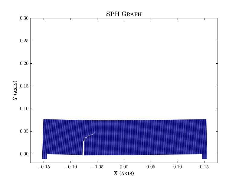
dv 1
                                                = ∇σ                                              (2)
                                              dt ρ
                                         de 1
                                           = σ : (∇ ⊗ v)                                          (3)
                                         dt ρ
where ρ denotes the material density, v and σ are respectively the velocity vector and Cauchy
stress tensor in the current configuration, e is the specific internal energy, d/dt is time derivative
taken in a moving Lagrangian frame. ∇ denotes the divergence or gradient operator, and ⊗ is the
outer product between two vectors.
    In this section, the TLSPH formulation [26, 44, 45, 46, 47] of particle approximation and
conservation equations are discussed briefly. In the total Lagrangian description of SPH, the con-
servation and the constitutive equations are solved in the undeformed or reference configuration X
only. The changes in the field variables are used to compute the current deformed configuration x.
The current description x is related to the reference description X through a mapping φ as

                                             x = φ (X, t)                                         (4)
   The displacement u is computed as

                                              u= x−X                                              (5)
    The mass, momentum and energy conservation equation 1, 2 and 3 [44] can be expressed in
terms of the reference configurations as follows

                                              ρ = J −1 ρ0                                         (6)

                                           dv  1
                                              = ∇0 · P                                            (7)
                                           dt ρ0
                                           de  1
                                              = P : Ḟ                                            (8)
                                           dt ρ0
where, 0 indicates that the values are computed at the undeformed reference configuration X, P
denotes the first Piola Kirchhoff stress, J is the Jacobian computed as J = det(F), where F denotes
the deformation gradient matrix calculated as
                                              dx    du
                                         F=       =     +I                                      (9)
                                             dX dX
    The deformation gradient matrix F relates the current and reference configuration, i.e. it de-
fines the deformation of a line element in the current configuration based on the reference config-
uration. I is an identity tensor.

                                                  4
2.1. Particle approximation in TLSPH
In TLSPH, any field variable f (Xi ) is approximated based on the reference configuration as
follows
X mj
f (Xi ) = f (X j )W(Xi j ) (10)
j
ρ 0 j
where f (X j ) is the field variable value at j-th particle, Xi j = Xi − X j is the vector from particle j to
particle i, m j /ρ0 j represents the volume of j-th particle in the reference configuration and W(Xi j ) is
the kernel function defined in the undeformed reference configuration. In this work, the following
cubic B spline function is used for the approximation.
3 3
1 − q2 + q3 , if 0 ≤ q ≤ 1
1 2 4
W(q, h) = αd 3
(2 − q) , if 1 ≤ q ≤ 2 (11)
4
0
otherwise
where, αd = 10/7πh2 in 2D and q = |Xi − X j |/h is the normalised distance associated with a
particle pair with smoothing length h.
The derivative of the function f (Xi ) is approximated as
X mj
∇ f (Xi ) = f (X j )∇i W(Xi j ) (12)
j
ρ0 j
where ∇i W(Xi j ) is the kernel derivative computed at Xi based on the reference configuration.
Monaghan [48] suggested symmetric approximation form for the zeroth order completeness in the
derivative approximation with the Eulerian kernel. Similarly, the symmetric estimate for derivative
approximation in TLSPH writes as follows
Xh i mj
∇ f (Xi ) = − f (Xi ) − f (X j ) ∇i W(Xi j ) (13)
j
ρ0 j
Consequently, the particle approximation form for the deformation gradient and its rate are
X mj X mj
Fi = − ui − u j ⊗ ∇i W(Xi j ) +I=− xi − x j ⊗ ∇i W(Xi j ) (14)
j
ρ0 j j
ρ0 j
X mj
Ḟi = − vi − v j ⊗ ∇i W(Xi j ) (15)
j
ρ0 j
The conservation equations 7 and 8 can be expressed in particle form as
dvi X Pi Pj
= m j 2 + 2 − Πi j ∇i W(Xi j ) (16)
dt j
ρ0i ρ0 j
dei Pi X mj
= : vi − v j ⊗ ∇i W(Xi j ) (17)
dt ρ0i j
ρ0 j
5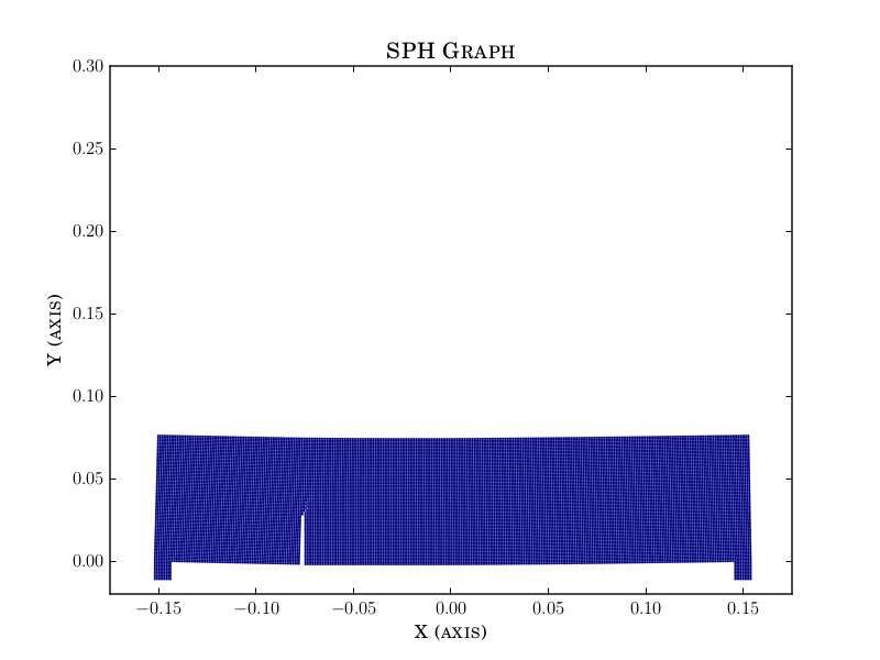
where, the first Piola Korchhoff stress P is calculated as P = JF−1 σ. Πi j is the artificial viscosity
computed as Πi j = JF−1 πi j . In the presence of jump in field variables or shock, the artificial
viscosity is used to for stabilised SPH computation. In the present work, the artificial viscosity
[49] is used in the following form.
−β1C̄i j µi j + β2 µ2i j
, if vi j · xi j ≤ 0
πi j = (18)
ρ̄i j
0, otherwise
where, β1 , β2 are the controlling parameters for artificial viscosity, µi j = h(vi j · xi j )/(x2i j + ǫh2 ); ǫ is
p
a small number used to avoid singularity (here ǫ = 0.01), sound speed is computed as C = E/ρ
in the materials, E is the Young’s modulus, xi j = xi − x j , vi j = vi − v j , C̄i j = (Ci + C j )/2
and ρ¯i j = (ρi + ρ j )/2. The controlling parameters of artificial viscosity β1 and β2 are obtained
through numerical experiments so that the fluctuations due to the shock or jump present in the
field variables are removed without over damping the computation.
2.2. Constitutive model
The Cauchy stress σ is computed based on the hydrostatic pressure p and the deviatoric stress
s as σ = s − pI. Material frame invariant Jaumann stress rate is used to compute the deviatoric
stress components as
!
1
ṡ = 2µ ǫ̇ − ε̇I + sω − ωs (19)
3
where, µ is the shear modulus of the material; ǫ̇ and ω are the strain rate tensor and spin tensor, ε̇
is the sum of the diagonal components of the strain rate tensor. The strain rate and spin tensors are
obtained from the velocity gradient tensor l = ḞF−1 as
1
ǫ̇ = l + lT (20)
2
1
ω= l − lT (21)
2
In the present work, the linear function of compressibility [50] is used to compute the pressure
p as, !
ρ
p=K −1 (22)
ρ0
where K = E/(3 − 6ν) is the bulk modulus, ν is the poison’s ratio of the material.
The material plasticity is incorporated by the pressure-independent
√ √ Von-Mises yield criterion,
in which the yield function is defined as y f = J2 − σy / 3, where σy is the yield stress of
material and J2 = s : s/2 is the second invariant of the deviatoric stress tensor. Return mapping
algorithm to bring back the deviatoricstress√ to theyield surface is implemented using the Wilkins
criterion as sn = c f s, where c f = min σy / 3J2 , 1 and sn is the corrected deviatoric stress tensor.
6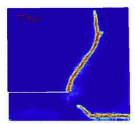
The following equations compute the increment of plastic strain, the increment of effective plastic
strain and the accumulated plastic work density
                                                         1 − cf
                                               ∆ǫ pl =          s                                 (23)
                                                           2µ
                                        r                              r
                                            2                 1 − cf       3
                              ∆ǫ pl =         ∆ǫ pl : ∆ǫ pl =                s:s                  (24)
                                            3                   3µ         2

                                              ∆w p = ∆ǫ pl : sn                                   (25)

3. Treatment for material damage and fracture
    When solid materials undergo large deformation, the adjacent material points will always re-
main as neighbour points unless the body has crack surfaces formed and loses continuity. Trans-
lating this condition into an SPH point of view, a particle should always interact with the same
set of neighbouring particles. However, this requirement is not satisfied in standard SPH. On the
other hand, in TLSPH the particle interactions are computed based on the initial configuration,
where the deforming property of solids is naturally modelled. However, the original form of TL-
SPH cannot handle problems with explicit material separation such as cracking and fragmentation,
as the material is always treated as a continuous body because the particle connectivity is fixed.
Therefore, the original form of TLSPH is incapable of modelling material damage. Additional
treatment is needed to model discontinuities such as cracking surface.
    A pseudo-spring analogy for modelling cracks and damage in solid materials in standard SPH
with immediate neighbour interaction is proposed in [33]. The algorithm is extended in modelling
of crack paths and their interaction for brittle and ductile materials in [35, 36, 37, 38]. How-
ever, the major disadvantage of this approach is that it suffers from tensile instability. The artifi-
cial/Monaghan pressure is used in that computational framework to overcome tensile instability.
However, the artificial/Monaghan pressure coefficient needs to be determined through numerical
calibrations for each problem. As TLSPH avoids tensile instability, TLSPH is an appropriate
method for cracking modelling in solids.
    In SPH, the bell-shaped kernel functions ensure that the influence of particles inversely varies
with the distance from the particle of interest, i.e. the influence of the immediate neighbour parti-
cles is at maximum whereas the influence of the particles near the kernel boundary is minimum.
This property of the kernel function inspires the assumptions of the present cracking treatment
method. In the present method, the neighbour definition of particles is modified, where a particle
only interacts with its immediate neighbours as shown in Figure 1.
    Moreover, the particles are connected through a set of virtual links. These links are termed
“virtual” because they do not provide any extra stiffness to the system but only defines the level of
interaction between particles. The material constitutive properties guide the damage evolution of
these links and consequently define the interaction. In the initial stage, as there is no damage in the
links, the particles interact normally without any reduction. As the material deforms, the damage
index increases in these links, resulting in reduced interaction between connecting particles. The

                                                         7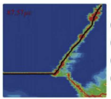
interaction between particles ceases to exist once the link is completely damaged and it is assumed
that the crack path propagates through that damaged link as shown in Figure 1. With the help of
the virtual link, the complete crack path can be tracked automatically through these damaged links
(Figure 1). The presented method avoids the use of particle splitting or visibility criterion; thus, it
simplifies the formulation and implementation and reduces the computational cost.
                    Full kernel support                                               Crack path


           Virtual links connect   Interaction of par
           ing immediate neigh     ticle i restricted to                 Propagation of cracks tracked
           bour particles           immediate neigh                      through damaged virtual links
                                    bour particles

                                                            Undamaged virtual links

                                                            Damaged virtual links

         Figure 1: Virtual links on immediate neighbours and crack propagation through damaged links

3.1. Consistency correction
    As the neighbour is redefined in the present algorithm, but the smoothing length is kept un-
changed, the approximation might not preserve the zeroth- or first-order consistency. Hence, a
gradient correction as proposed in [23] is employed to restore the consistency in the approxima-
tion as follows.

                                              ∇i Ŵ(Xi j ) = Ki ∇i W(Xi j )                               (26)
where,                                                              X                         mj
                            Ki = B−1
                                  i , where Bi = −                       Xi j ⊗ ∇i W(Xi j )               (27)
                                                                     j
                                                                                              ρ0 j
   This correction also removes the truncation error caused by the incomplete support domain.

                                                               8
3.2. Modified conservation equations
An interaction coefficient fi j is introduced to define the state of interaction between the particle
pair i and j. The computation of fi j is purely based on the damage index Di j of the particle pair as
f i j = 1 − Di j (28)
Initially, the material is assumed to be undamaged i.e. Di j = 0. This means complete interaction
between the particle pair or fi j = 1. Once failure starts, the damage index Di j increases, thus fi j
becomes less than 1, implying partial or reduced interaction between particles (0 < Di j < 1 i.e.
0 < fi j < 1). When the damage index Di j reaches 1, fi j becomes 0 (Equation 28). This implies a
broken link, i.e., the interaction between the connecting particles through the broken link ceases
to exist completely. Therefore, a discontinuous crack surface is implicitly modelled through the
broken link.
The interaction function fi j is multiplied with the corrected kernel ∇i W̄(Xi j ) = fi j ∇i Ŵ(Xi j ).
The shapes of the modified kernel function W̄(Xi j ) and its derivative ∇i W̄(Xi j ) for different in-
teraction coefficients fi j are shown in Figure 2. Let N i be the set of particles in the modified
neighbourhood of particle i in the reference configuration. NUi and NDi are the sets of neighbouring
particles connected to the particle i through the undamaged and damaged virtual links, respec-
tively. The damage index Di j is zero and the interaction coefficient fi j is one for the particles in the
set NUi . Similarly, for the particles in the set NDi , 0 < Di j ≤ 1 and 1 > fi j ≥ 0 hold. In short, fi j = 1
means no damage, 0 < fi j < 1 means partial damage and fi j = 0 means fully damaged virtual
link, or generation of new crack opening. With the modified kernel gradients, the conservation
equatons 16 and 17 accordingly have the following form
dvi X Pi Pj X Pi Pj
= m j 2 + 2 − Πi j ∇i Ŵ(Xi j ) + m j 2 + 2 − Πi j fi j ∇i Ŵ(Xi j )
(29)
dt i
ρ0i ρ0 j i
ρ0i ρ0 j
j∈NU j∈ND
dei Pi X mj Pi X mj
= : vi − v j ∇i Ŵ(Xi j ) + : vi − v j fi j ∇i Ŵ(Xi j ) (30)
dt ρ0i i
ρ0 j ρ0i i
ρ0 j
j∈NU j∈ND
4. Contact froce
An explicit contact algorithm is necessary for TLSPH to model the interaction between differ-
ent bodies due to the use of the reference configuration. In the present work, the pin-ball contact
algorithm as proposed in [51] is used to model the multi-body contact in TLSPH. In this approach,
it is assumed that each SPH particle is a virtual contact body, which is a circle in 2D and a sphere
in 3D, having a radius of kh, where k is a constant factor. Once the virtual contact bodies of the
particles belonging to different objects overlap each other, the contact is activated as shown in
Figure 3. The material properties and the relative motions of the objects in contact determine the
contact force.
For a particle pair i- j, the magnitude of the overlapping is determined as
pd = (Ri + R j ) − |xi − x j | (31)
9(a) Kernel: fi j = 1 (b) Kernel: 0 < fi j < 1 (c) Kernel: fi j = 0
(d) Derivative: fi j = 1 (e) Derivative: 0 < fi j < 1 (f) Derivative: fi j = 0
Figure 2: Modification of kernel in 2D based on damage state of virtual links
10Radius of inuence of particle
j
j
No penetration between particles
Penetration between particles
i i
Figure 3: Penetration between particles for contact force
where, Ri and R j are the radii of the virtual contact bodies of i-th and j-th particle, respectively.
pd > 0 means there is overlap between the two bodies. As a result, the contact force between the
particle pair is evaluated [52] as
F i j = K p min(F i1j , F i2j ) (32)
where,
ρi ρ j R3i R3j p˙d
, p˙d > 0
F i1j =
3
ρi Ri + ρ j R3j ∆t (33)
0,
p˙d < 0
s
µi µ j R i R j
F i2j = p1.5 (34)
µi + µ j Ri + R j d
where ∆t is the time step, p˙d = |vi − v j | is the rate of penetration and K p is a scale factor gener-
ally chosen (through numerical experiment) based on particle spacing, impact velocity etc. The
modified momentum equation 29 is modified by including the contact force
!
dvi dvi xi − x j F i j
= + (35)
dt dt Eq. 29 |xi − x j | mi
5. Numerical simulation
In this section, the performance of the proposed TLSPH method with the virtual link is inves-
tigated. The numerical results are compared with analytical, numerical, and experimental results
available in the literature. Four cases, i.e., the deflection of a beam under impact, the crack prop-
agation in a notched beam, the Kalthoff-Winkler experiment, and different modes of failure in a
deep beam are modelled. Overall, the results are found to be in good agreement with the reference
results. The present approach does not introduce unphysical numerical fracture or failure in the
computation.
115.1. Rigid-Plastic analysis for perfect beam
Unconventional particle connectivity is used in the presented method because only the imme-
diately neighbouring particles are considered in the simulation. To assess the influence of this,
firstly, the midpoint deflection of an Aluminium beam is modelled. The beam is of 142.24 mm
length; the cross-section is 6.35 mm × 6.35 mm. In the experiment, it is deflected under the impact
of a cylindrical projectile of 50 mm length and 14.74 mm diameter [53]. The case is idealised into
a 2D problem with unit width. The mass of the projectile is scaled [36] to keep the mass ratio
between the projectile and target the same and to keep the transmitted impulse constant. The ma-
terial parameters for the beam and projectile are shown in Table 1. The stiffness and yield stress of
the projectile is much higher than those of the beam. Consequently, the deformation of the projec-
tile is negligible. It behaves almost like a rigid body in this simulation. Therefore, the analytical
solution of the deflection at the midpoint of the beam in [54] can be used as a reference solution,
which reads
Table 1: Material parameters for the steel projectile and the aluminium beam.
ρ (kg/m3 ) E (GPa) ν σy (MPa)
Steel projectile 7850 200 0.3 600
Aluminum beam 2680 68.95 0.33 277.8
Width
im)
Impactor
Mass G)
Fixed
Target beam
support
Free length 2L)
Figure 4: Clamped aluminium beam struck by a steel projectile at the mid-span.
s
wf 1 GV 2 L/(M p H)
= −1 + 1 + (36)
H 2 1 + L/(2L − L)
where G is the mass of the projectile; L is the distance between the impact location to the support
with 2L the length of the free part of the beam; H is the thickness of the beam; M p = 0.25σy BH 2
is the plastic moment of the beam, where B is the width and σy is the yield stress; and v0 is the
initial velocity of the projectile.
12Four simulations with different particle discretisation are performed using the presented TL-
SPH method. Impact velocity of 20 m/s is considered in these four simulations. The midpoint
defection of the aluminium beam is compared with the values obtained from the analytical solu-
tion, as shown in Figure 5. The present approach demonstrates monotonous convergence. The
history of the deflection in the simulation with ∆p = 0.423 mm is shown in Figure 6. The elastic
oscillation of the beam is observed. The accumulated equivalent plastic strain at different locations
for the 20 m/s impact velocity case is shown in Figure 7. The deformation pattern and distribution
of the plastic strain are well captured using the presented method.
To measure the effect of impact energy, another four simulations with fixed particle discretisa-
tion (∆p = 0.423 mm) but varying impact velocity are carried out. The deflection at the midpoint
is shown in Figure 8.
Although only immediate neighbouring particles are considered in the simulation, it is found
that the numerical results are well corroborated by the analytical solution. Furthermore, good con-
vergence behaviour is observed. This is mainly because of the kernel gradient correction which
restores the first-order consistency. Thus, the truncated kernel interaction does not lead to unphys-
ical behaviour.
Figure 5: Normalised permanent displacement for different discretisation with present formulation (v0 = 20 m/s).
5.2. Crack propagation in notched beam
Chen and Yu [53] analysed the crack propagation and failure of beams with initial notches of
different sizes and locations. In this section, several representative beams are selected and mod-
elled using the present approach. The capabilities of the scheme to predict the crack propagation,
plastic strain accumulation and failure are tested. The details of the notch are shown in Figure
9. Three different notch dimensions are used - Type I (WN = 0.8 mm; DN = 2.12 mm), Type II
(WN = 1.5 mm; DN = 2.12 mm) and Type III (WN = 0.8 mm; DN = 1.59 mm). The material
parameters are the same as those used in Section 5.1 given in Table 1. The damage in the virtual
links is calculated based on the accumulated plastic strain, which is obtained by transferring the
plastic strain from the particles to the links, as illustrated in Figure 10. Firstly, the plastic strain is
13Figure 6: Deflection for the midpoint of the aluminium beam (∆p = 0.423 mm, v0 = 20 m/s)
(a) Time = 0.1 ms (b) Time = 0.5 ms
(c) Time = 1.0 ms (d) Time = 1.5 ms
Plastic Strain: 0 0.01 0.02 0.03 0.04 0.05 0.06 0.07 0.08 0.09 0.1
Figure 7: Accumulation of plastic strain at different time step (∆p = 0.423 mm, v0 = 20 m/s)
14Figure 8: Transverse deflection at mid-span for different velocities (∆p = 0.423 mm).
rotated to the local coordinate systme R-S (R and S are the axes that are parallel and perpendicular
to the considered virtual link, respectively) [36]
yy
x2i j ǫ plxx |i + y2i j ǫ pl |i + 2xi j yi j ǫ plxy |i
RR
ǫ pl |i = TR ǫ pl |i TRT = (37)
x2i j + y2i j
where TR = [−xi j /(x2i j + y2i j ), − yi j /(x2i j + y2i j ]. Then the value of plastic strain at the virtual link i- j
RR
(ǭ pl |i j ) in the R direction is calculated as the average value of particle i and j (equation 38)
RR RR
RR
ρiCi ǫ pl | j + ρ jC j ǫ pl |i
ǭ pl |i j = (38)
ρi C i + ρ j C j
RR
The relation between the damage index D and the plastic strain in the virtual link ǭ pl |i j is
given in equation 39, where (ǫ pl )max is a material parameter taken as 0.17 in this work [55]. The
employed relation indicates a sudden cracking; however, more sophisticated cracking criterion can
be used in the current framework.
Notch width W )
Notch
depth
)
Figure 9: Location and geometry of the notch for the clamped aluminium beam
1,
ǫ pl ≥ (ǫ pl )max
D= (39)
0,
otherwise
First, the beams with midpoint notches are modelled. The deformation and failure patterns
are compared with the experimental results from [53] in Figure 11. Large plastic deformation can
15Y
S
X
pl j
Y RR
pl ij
irtual link
X
pl i
Figure 10: Effective plastic strain in the virtual link
be observed near the notch and the support. As the notch becomes wider and the impact velocity
higher, the deflection increases with a higher plastic deformation near the notch. The cracking
initiates at the tip of the notch and propagates deeper into the beam with increasing notch width
and impact velocity. With impact velocity v0 = 27.1 m/s, a complete failure is observed where the
left and right parts of the beam separate completely (Figure 11g, 11h).
All the results from the simulation with a notch at the midpoint are summarised in Table 2.
It is found that for different notch types and impact velocities, the overall agreement between the
numerical and experimental results are good. The deflection, deformation pattern and cracking
propagation are correctly captured using the presented method. Importantly, the present method
does not use any enrichment or geometry-based treatment. The crack propagation and material
separation are modelled naturally without complex formulation or implementation.
Table 2: Summary of the results from simulations with notches at the midpoint
Notch type I I II II
Initial velocity (m/s) 14.2 18.2 19.2 27.1
Experimental deflection (mm) 7.92 8.62 10.18 NA
Numerical deflection (mm) 6.29 8.65 9.01 NA
Experimental observation LN and CI LN and just B LN and just B B
Numerical observation LN and CI LN and just B LN and just B B
NA: Not apply
LN: Local necking
CI: Crack initiated
B: Broken completely at notch location
Next, the beams with notches at the two supports are considered. Three simulations with
type III and I notch and different velocities are performed. The deformation modes are compared
with the experimental observation in Figure 12. The contour of effective plastic strains is also
given. Table 3 summaries the numerical results from all the simulations. The simulation with
31.6 m/s impact velocity shows complete failure near the supports, while other beams in the other
two simulations undergo large plastic deformation and initial cracking. These numerical results
16(a) 14.2 m/s (Experimental) (b) 14.2 m/s (Present simulation)
(c) 18.2 m/s (Experimental) (d) 18.2 m/s (Present simulation)
(e) 19.2 m/s (Experimental) (f) 19.2 m/s (Present simulation)
(g) 27.1 m/s (Experimental) (h) 27.1 m/s (Present simulation)
Plastic Strain: 0 0.01 0.02 0.03 0.04 0.05 0.06 0.07 0.08 0.09 0.1
Figure 11: Comparison of present simulation with the experimental observation [53]
17are consistent with the experimental observations. Therefore, it can be observed that the present
formulation performs well in predicting the permanent deflection, crack initiation, plastic strain
accumulation, crack propagation and failure.
(a) 18.5 m/s (Experimental) (b) 18.5 m/s (Present simulation)
(c) 17.7 m/s (Experimental) (d) 17.7 m/s (Present simulation)
(e) 31.6 m/s (Experimental) (f) 31.6 m/s (Present simulation)
Plastic Strain: 0 0.01 0.02 0.03 0.04 0.05 0.06 0.07 0.08 0.09 0.1
Figure 12: Comparison of present simulation with the experimental observation [53]
5.3. Kalthoff-Winkler numerical experiments
For the third example, the crack propagation from Kalthoff-Winkler [56] is simulated. A
double-notched target is subjected to an impact loading, then crack initiates at the tip of the notch
and propagates at an angle of 70◦ . The geometry and boundary condition of the experiment are
shown in Figure 13a. Owing to the symmetricity of the geometry, only half of the specimen is
modelled. The symmetric boundary condition is employed, as shown in Figure 13b.
The material and computational parameters are shown in Table 4 and 5. The material is as-
sumed to be elastic. The following Rankine criterion is used for the damage evolution
ri j |t − ri j |t0
1, ≥ ǫmax
D= r i j | t0 (40)
0, otherwise
18Table 3: Summary of the results from simulations with notches at the supports
Notch type III I I
Initial velocity (m/s) 18.5 17.7 31.6
Experimental deflection (mm) 7.55 7.07 NA
Numerical deflection (mm) 6.72 6.70 NA
Experimental observation PD, LN and just CI Small PD, LN and CI B
Numerical observation PD, LN and just CI Small PD, LN and CI B
NA: Not apply
PD: Plastic deformation
LN: Local necking
CI: Crack initiated
B: Broken completely at notch location
1 mm
5 mm 2 mm
5 mm
75 mm 1 mm
75 mm
25 mm 25 mm
1 Symmetric boundary condition
(a) (b)
Figure 13: Initial set-up for the Kalthoff-Winkler experiment
19where ri j |t and ri j |t0 are the interparticle distances between the i-th and j-th particles at the refer-
ence and the current configurations. The criterion indicates a brittle failure once the deformation
between two particles is larger than the threshold. Similar cracking criterion is employed in other
particle-based methods such as peridynamics [57] and the smoothed particle Galerkin method
(SPG) [58].
Table 4: Material parameters for crack propagation in the deep beam
Mechanical properties Failure parameter
ρ = 8000 kg/m3 ǫmax = 0.0044
E = 190 GPa (for Rankine criterion)
ν = 0.3
Table 5: Computational parameters used for Kalthoff-Winkler
∆p (mm) h (mm) β1 β2
0.5 0.65 0.5 0.5
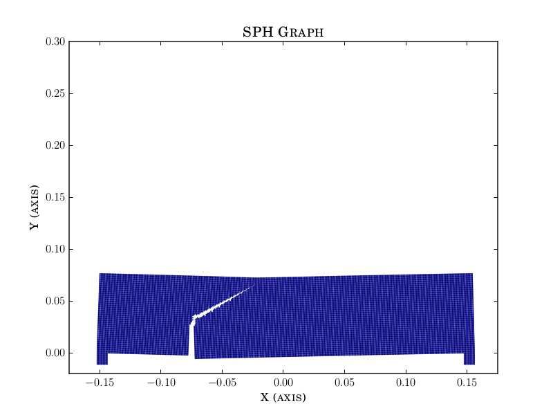
The dynamic crack propagation at different time step is shown in Figure 14. Under the impact
loading, a crack initiates at the tip of the notch and propagates to the edge of the boundary. The
angle of the whole cracking path is approximately 77◦ , close to the cracking angle obtained in the
test and other numerical simulations. The averaged damage index D is also shown in Figure 14,
P
which is obtained as Di = ( j Di j )/n, where Di j is the damage index of the virtual link between
particle i and j, and n is the number of particles in the modified support domain of particle i.
As this cracking problem is investigated using several other numerical methods with various
cracking or damage criterion, the obtained crack path is compared with experimental and other
numerical approaches in Figure 15. In some of the numerical simulations a secondary crack path
is also observed as shown in Figure 15b, 15c, 15f, 15g, which is not present in the experimental ob-
servation (Figure 15a). The present approach captures the crack path without any secondary crack
paths (Figure 15h). Among all the numerical results, there are discrepancies regarding the crack-
ing path and curve shape, which are mainly caused by different cracking criteria. Furthermore,
some of the numerical results are obtained using a crack tracking algorithm, which we do not em-
ploy in this work. Therefore, our numerical results show a certain degree of particle distribution
dependency. Nevertheless, this example demonstrates the capability of the present algorithm to
capture the crack initiation and propagation at low strain rates.
5.4. Crack propagation in deep beams
As the last example, a simply supported deep beam with the notch at different location [64, 33]
is chosen (Figure 16) to demonstrate the capabilities of the present solution to capture the different
crack propagation and failure modes. A beam of 308 mm length and 76 mm depth is considered
under the impact of a projectile with 20 m/s velocity. The material and computational parameters
20(a) Time = 55.0 µs (b) Time = 70.0 µs
(c) Time = 90.0 µs (d) Time = 115.0 µs
Damage: 0.1 0.2 0.3 0.4 0.5 0.6 0.7 0.8 0.9
Figure 14: Damage evolution for the Kalthoff-Winkler experiment at different time step
21(a) Kalthoff-Winkler [56] (b) Kosteski et al. [59]
(c) Dipasquale et al. [60] (d) Huespe et al. [61]
(e) Chakraborty and Shaw [33] (f) Belytschko et al. [62]
22
(g) Zhou et al. [63] (h) Present study
Figure 15: Comparison of fianl crack propagation pathsare shown in Table 6 and 7. The notches are located at the midpoint and a distance of 75 mm from
the left support.
2 5 X mass of target 2 5 X mass of target
76 mm 76 mm
30 mm 30 mm
152 mm 152 mm
34 mm 34 mm
(a) Notch at mid-point (b) Notch away from mid-point
Figure 16: Set-up of the deep beam under impact with the notch at different locations
Table 6: Material parameters for crack propagation in deep beams
Mechanical properties Failure parameter
ρ = 7830kg/m3 ǫmax = 0.03
E = 200GPa (for Rankine criterion)
ν = 0.3
Table 7: Computational parameters used for deep beam
Inter-Particle Smoothing Artificial Viscosity
Spacing (∆ p) Length (h) Parameters (β1 , β2 )
1.0 mm 0.65 mm (2.0,2.0)
As reported in [64, 33], the beam undergoes elastic bending, and as a result, the crack starts
propagation from the notch tip. For the beam with the notch at the midpoint, the crack propagates
vertically leading to mode I failure. The crack propagation at different time step can be observed
in Figure 17. The crack path captured in the present study is compared with the results from [33]
in Figure 18. It can be observed that the crack propagates vertically from the notch edge. On
the other hand, for the beam with the notch away from the midpoint, a mixed mode type of crack
propagation is found due to the combined influence of shear and transverse tension. The mixed
mode crack propagation at different time step is shown in Figure 19. This is found to be consistent
with the observations in [33] as shown in Figure 20. Hence the present observations are consistent
with the results in [64, 33].
6. Conclusion
In TLSPH, the computations are based on the reference framework; thus, it is free from tensile
instability. This makes it a perfect candidate to model crack initiation, propagation and material
23(a) Time = 0.0 ms (b) Time = 0.5 ms
(c) Time = 0.6 ms (d) Time = 0.7 ms
Figure 17: Crack propagation in mode I (notch at mid-point) at different time step
(a) Chakraborty and Shaw [33] (b) Present Study
Figure 18: Comparison of crack path in mode I (notch at mid-point)
(a) Time = 0.0 ms (b) Time = 0.75 ms
(c) Time = 0.6 ms (d) Time = 1.0 ms
Figure 19: Crack propagation in mixed mode (notch away from mid-point) at different time step
(a) Chakraborty and Shaw [33] (b) Present Study
Figure 20: Comparison of crack propagation in mixed mode (notch away from mid-point)
24failure. TLSPH in its original form cannot capture the forming and development of discontinuities
as it is a continuum-based method. To provide a way out, a virtual link approach is proposed in the
framework of TLSPH. In this approach, the particle’s kernel support is modified to its immediate
neighbour. A network of virtual links connects the particles. These links are called virtual as they
do not provide any extra stiffness to the system but only defines the level of interaction between
the connecting particles. Initially, due to the absence of any material damage, the links allows
complete interaction. However, as the damage develops, the level of interaction is reduced between
the connecting particles. When the connection is completely damaged, the interaction between
particles stops, and the link is considered to be broken, implying the generation of a crack surface.
The material constitutive models and cracking criteria guide the damage variables of the links.
The proposed method is employed to model the crack initiation, propagation and failure of
notched beams under impact. The accumulation of plastic strain, initialisation of cracking and
ultimate failure are well captured using the present approach. The proposed model is also able
to simulate the brittle failure at low strain rates (Kalthoff-Winkler experiment) and the different
modes of crack propagations in a deep beam. As the damage and failure are considered using the
virtual links, the method does not need any cracking treatments such as particle deleting, splitting
or visibility criterion. The initialisation and propagation are naturally modelled. The present
method is observed to be stable in all the simulations.
Moreover, the crack path/surfaces can be tracked quite easily by monitoring the broken virtual
links. There is no need for any explicit crack tracking algorithm. Therefore, the computational
cost of the present framework is low, and the implementation is straightforward. Based on the
current investigation, the method seems to be entirely natural in tracking crack paths and failure
of solids. In the future, the approach will be explored for more complex brittle and ductile failure
modes with arbitrary material flaws.
Acknowledgement
This work receives funding from the European Unions Horizon 2020 programme under grant
agreement No. 778627 and the Austrian Research Promotion Agency (FFG) under the project No.
865963.
References
[1] T. Belytschko, On difficulty levels in non linear finite element analysis of solids, IACM expressions 2 (1996)
6–8.
[2] L. F. Martha, P. A. Wawrzynek, A. R. Ingraffea, Arbitrary crack representation using solid modeling, Engineer-
ing with Computers 9 (2) (1993) 63–82.
[3] J. M. Melenk, I. Babuška, The partition of unity finite element method: basic theory and applications, Computer
methods in applied mechanics and engineering 139 (1-4) (1996) 289–314.
[4] A. De-Andrés, J. Pérez, M. Ortiz, Elastoplastic finite element analysis of three-dimensional fatigue crack growth
in aluminum shafts subjected to axial loading, International Journal of Solids and Structures 36 (15) (1999)
2231–2258.
[5] T.-P. Fries, T. Belytschko, The extended/generalized finite element method: an overview of the method and its
applications, International Journal for Numerical Methods in Engineering 84 (3) (2010) 253–304.
[6] S. Li, W. K. Liu, Meshfree and particle methods and their applications, Applied Mechanics Reviews 55 (1)
(2002) 1–34.
25[7] R. A. Gingold, J. J. Monaghan, Smoothed particle hydrodynamics: theory and application to non-spherical stars,
Monthly notices of the royal astronomical society 181 (3) (1977) 375–389.
[8] L. B. Lucy, A numerical approach to the testing of the fission hypothesis, The astronomical journal 82 (1977)
1013–1024.
[9] M. Liu, G. Liu, Smoothed particle hydrodynamics (sph): an overview and recent developments, Archives of
computational methods in engineering 17 (1) (2010) 25–76.
[10] J. J. Monaghan, J. C. Lattanzio, A refined particle method for astrophysical problems, Astronomy and astro-
physics 149 (1985) 135–143.
[11] J. J. Monaghan, An introduction to sph, Computer physics communications 48 (1) (1988) 89–96.
[12] J. Monaghan, On the problem of penetration in particle methods, Journal of Computational physics 82 (1) (1989)
1–15.
[13] J. J. Monaghan, Simulating free surface flows with sph, Journal of computational physics 110 (2) (1994) 399–
406.
[14] L. D. Libersky, A. G. Petschek, Smooth particle hydrodynamics with strength of materials, in: Advances in
the free-Lagrange method including contributions on adaptive gridding and the smooth particle hydrodynamics
method, Springer, 1991, pp. 248–257.
[15] L. D. Libersky, A. G. Petschek, T. C. Carney, J. R. Hipp, F. A. Allahdadi, High strain lagrangian hydrodynamics:
a three-dimensional sph code for dynamic material response, Journal of computational physics 109 (1) (1993)
67–75.
[16] J. Swegle, D. Hicks, S. Attaway, Smoothed particle hydrodynamics stability analysis, Journal of computational
physics 116 (1) (1995) 123–134.
[17] T. Belytschko, Y. Guo, W. Kam Liu, S. Ping Xiao, A unified stability analysis of meshless particle methods,
International Journal for Numerical Methods in Engineering 48 (9) (2000) 1359–1400.
[18] P. Randles, L. Libersky, Normalized sph with stress points, International Journal for Numerical Methods in
Engineering 48 (10) (2000) 1445–1462.
[19] P. Randles, L. Libersky, Smoothed particle hydrodynamics: some recent improvements and applications, Com-
puter methods in applied mechanics and engineering 139 (1-4) (1996) 375–408.
[20] J. J. Monaghan, Sph without a tensile instability, Journal of Computational Physics 159 (2) (2000) 290–311.
[21] J. Gray, J. Monaghan, R. Swift, Sph elastic dynamics, Computer methods in applied mechanics and engineering
190 (49-50) (2001) 6641–6662.
[22] C. Dyka, R. Ingel, An approach for tension instability in smoothed particle hydrodynamics (sph), Computers &
structures 57 (4) (1995) 573–580.
[23] J. Chen, J. Beraun, T. Carney, A corrective smoothed particle method for boundary value problems in heat
conduction, International Journal for Numerical Methods in Engineering 46 (2) (1999) 231–252.
[24] T. Belytschko, S. Xiao, Stability analysis of particle methods with corrected derivatives, Computers & Mathe-
matics with Applications 43 (3-5) (2002) 329–350.
[25] T. Rabczuk, T. Belytschko, S. Xiao, Stable particle methods based on lagrangian kernels, Computer methods in
applied mechanics and engineering 193 (12-14) (2004) 1035–1063.
[26] R. Vignjevic, J. R. Reveles, J. Campbell, Sph in a total lagrangian formalism, CMC-Tech Science Press- 4 (3)
(2006) 181.
[27] J. Bonet, S. Kulasegaram, Alternative total lagrangian formulations for corrected smooth particle hydrodynamics
(csph) methods in large strain dynamic problems, Revue Européenne des Éléments Finis 11 (7-8) (2002) 893–
912.
[28] T. Rabczuk, T. Belytschko, Cracking particles: a simplified meshfree method for arbitrary evolving cracks,
International Journal for Numerical Methods in Engineering 61 (13) (2004) 2316–2343.
[29] T. Rabczuk, T. Belytschko, A three-dimensional large deformation meshfree method for arbitrary evolving
cracks, Computer Methods in Applied Mechanics and Engineering 196 (29-30) (2007) 2777–2799.
[30] T. Rabczuk, G. Zi, S. Bordas, H. Nguyen-Xuan, A simple and robust three-dimensional cracking-particle method
without enrichment, Computer Methods in Applied Mechanics and Engineering 199 (37-40) (2010) 2437–2455.
[31] D. Organ, M. Fleming, T. Terry, T. Belytschko, Continuous meshless approximations for nonconvex bodies by
diffraction and transparency, Computational mechanics 18 (3) (1996) 225–235.
26[32] B. Ren, S. Li, Meshfree simulations of plugging failures in high-speed impacts, Computers & structures 88 (15-
16) (2010) 909–923.
[33] S. Chakraborty, A. Shaw, A pseudo-spring based fracture model for sph simulation of impact dynamics, Inter-
national Journal of Impact Engineering 58 (2013) 84–95.
[34] A. Shaw, S. Reid, D. Roy, S. Chakraborty, Beyond classical dynamic structural plasticity using mesh-free mod-
elling techniques, International Journal of Impact Engineering 75 (2015) 268–278.
[35] S. Chakraborty, A. Shaw, Crack propagation in bi-material system via pseudo-spring smoothed particle hydrody-
namics, International Journal for Computational Methods in Engineering Science and Mechanics 15 (3) (2014)
294–301.
[36] S. Chakraborty, A. Shaw, Prognosis for ballistic sensitivity of pre-notch in metallic beam through mesh-less
computation reflecting material damage, International Journal of Solids and Structures 67 (2015) 192–204.
[37] S. Chakraborty, M. R. I. Islam, A. Shaw, L. Ramachandra, S. Reid, A computational framework for modelling
impact induced damage in ceramic and ceramic-metal composite structures, Composite Structures 164 (2017)
263–276.
[38] M. R. I. Islam, S. Chakraborty, A. Shaw, S. Reid, A computational model for failure of ductile material under
impact, International Journal of Impact Engineering 108 (2017) 334–347.
[39] X. Zhou, Y. Zhao, Q. Qian, A novel meshless numerical method for modeling progressive failure processes of
slopes, Engineering Geology 192 (2015) 139–153.
[40] J. Bi, X.-P. Zhou, X.-M. Xu, Numerical simulation of failure process of rock-like materials subjected to impact
loads, International Journal of Geomechanics 17 (3) (2016) 04016073.
[41] J. Bi, X. Zhou, Numerical simulation of kinetic friction in the fracture process of rocks in the framework of
general particle dynamics, Computers and Geotechnics 83 (2017) 1–15.
[42] P. Yin, H. Ma, X. Liu, J. Bi, X. Zhou, F. Berto, Numerical study on the dynamic fracture behavior of 3d
heterogeneous rocks using general particle dynamics, Theoretical and Applied Fracture Mechanics 96 (2018)
90–104.
[43] M. Liu, G. Liu, Restoring particle consistency in smoothed particle hydrodynamics, Applied numerical mathe-
matics 56 (1) (2006) 19–36.
[44] T. De Vuyst, R. Vignjevic, Total lagrangian sph modelling of necking and fracture in electromagnetically driven
rings, International Journal of Fracture 180 (1) (2013) 53–70.
[45] G. C. Ganzenmüller, An hourglass control algorithm for lagrangian smooth particle hydrodynamics, Computer
Methods in Applied Mechanics and Engineering 286 (2015) 87–106.
[46] S. Leroch, M. Varga, S. Eder, A. Vernes, M. R. Ripoll, G. Ganzenmüller, Smooth particle hydrodynamics
simulation of damage induced by a spherical indenter scratching a viscoplastic material, International Journal of
Solids and Structures 81 (2016) 188–202.
[47] M. Rausch, G. Karniadakis, J. Humphrey, Modeling soft tissue damage and failure using a combined parti-
cle/continuum approach, Biomechanics and modeling in mechanobiology 16 (1) (2017) 249–261.
[48] J. J. Monaghan, Smoothed particle hydrodynamics, Annual review of astronomy and astrophysics 30 (1) (1992)
543–574.
[49] J. Monaghan, R. A. Gingold, Shock simulation by the particle method sph, Journal of computational physics
52 (2) (1983) 374–389.
[50] S. Eliezer, A. Ghatak, H. Hora, E. Teller, An introduction to equations of state: theory and applications, Cam-
bridge University Press, Cambridge, 1986.
[51] J. Campbell, R. Vignjevic, L. Libersky, A contact algorithm for smoothed particle hydrodynamics, Computer
methods in applied mechanics and engineering 184 (1) (2000) 49–65.
[52] T. Belytschko, I. Yeh, The splitting pinball method for contact-impact problems, Computer methods in applied
mechanics and engineering 105 (3) (1993) 375–393.
[53] F. Chen, T. Yu, An experimental study of pre-notched clamped beams under impact loading, International journal
of solids and structures 41 (24-25) (2004) 6699–6724.
[54] J. Liu, N. Jones, Experimental investigation of clamped beams struck transversely by a mass, International
Journal of Impact Engineering 6 (4) (1987) 303–335.
[55] S. Sen, A. Shaw, Analytical model for failure of clamped beam subjected to projectile impact, in: Recent
27Advances in Structural Engineering, Volume 2, Springer, 2019, pp. 161–172.
[56] J. Kalthoff, S. Winkler, Failure mode transition at high rates of shear loading, DGM Informationsgesellschaft
mbH, Impact Loading and Dynamic Behavior of Materials 1 (1988) 185–195.
[57] S. A. Silling, Reformulation of elasticity theory for discontinuities and long-range forces, Journal of the Me-
chanics and Physics of Solids 48 (1) (2000) 175–209.
[58] C. Wu, Y. Wu, Z. Liu, D. Wang, A stable and convergent lagrangian particle method with multiple nodal stress
points for large strain and material failure analyses in manufacturing processes, Finite Elements in Analysis and
Design 146 (2018) 96–106.
[59] L. Kosteski, R. B. DAmbra, I. Iturrioz, Crack propagation in elastic solids using the truss-like discrete element
method, International journal of fracture 174 (2) (2012) 139–161.
[60] D. Dipasquale, M. Zaccariotto, U. Galvanetto, Crack propagation with adaptive grid refinement in 2d peridy-
namics, International Journal of Fracture 190 (1-2) (2014) 1–22.
[61] A. Huespe, J. Oliver, P. Sanchez, S. Blanco, V. Sonzogni, Strong discontinuity approach in dynamic fracture
simulations, Mecánica Computacional 25 (2006) 1997–2018.
[62] T. Belytschko, H. Chen, J. Xu, G. Zi, Dynamic crack propagation based on loss of hyperbolicity and a new
discontinuous enrichment, International journal for numerical methods in engineering 58 (12) (2003) 1873–
1905.
[63] X. Zhou, Y. Wang, Q. Qian, Numerical simulation of crack curving and branching in brittle materials under
dynamic loads using the extended non-ordinary state-based peridynamics, European Journal of Mechanics-
A/Solids 60 (2016) 277–299.
[64] M. Ortiz, A. Pandolfi, Finite-deformation irreversible cohesive elements for three-dimensional crack-
propagation analysis, International journal for numerical methods in engineering 44 (9) (1999) 1267–1282.
28You can also read