Refinement of polygonal grids using Convolutional Neural Networks with applications to polygonal Discontinous Galerkin and Virtual Element methods
←
→
Page content transcription
If your browser does not render page correctly, please read the page content below
Refinement of polygonal grids
                                                   using Convolutional Neural Networks
arXiv:2102.05738v1 [math.NA] 10 Feb 2021

                                                with applications to polygonal Discontinous
                                                  Galerkin and Virtual Element methods∗
                                                                             P. F. Antonietti†
                                                                               E. Manuzzi†
                                                                           February 12, 2021

                                           Abstract
                                           We propose new strategies to handle polygonal grids refinement based on Con-
                                           volutional Neural Networks (CNNs). We show that CNNs can be successfully
                                           employed to identify correctly the “shape” of a polygonal element so as to
                                           design suitable refinement criteria to be possibly employed within adaptive re-
                                           finement strategies. We propose two refinement strategies that exploit the use
                                           of CNNs to classify elements’ shape, at a low computational cost. We test the
                                           proposed idea considering two families of finite element methods that support ar-
                                           bitrarily shaped polygonal elements, namely Polygonal Discontinuous Galerkin
                                           (PolyDG) methods and Virtual Element Methods (VEMs). We demonstrate
                                           that the proposed algorithms can greatly improve the performance of the dis-
                                           cretization schemes both in terms of accuracy and quality of the underlying
                                           grids. Moreover, since the training phase is performed off-line and is problem
                                           independent the overall computational costs are kept low.

                                           1     Introduction
                                           In the last years, there has been a great interest in developing polygonal finite
                                           element methods for the numerical discretizations of partial differential equa-
                                           tions. We mention the mimetic finite difference method [31, 15, 14, 8], the
                                           hybridizable discontinuous Galerkin methods [19, 22, 20, 21], the Polygonal
                                              ∗ P. F. Antonietti has been partially supported by PRIN grant n. 201744KLJL funded by

                                           MIUR. P. F. Antonietti and E. Manuzzi are members of INDAM-GNCS.
                                              † MOX, Dipartimento di Matematica, Politecnico di Milano, I-20133 Milano, Italy (paola.

                                           antonietti@polimi.it, enrico.manuzzi@polimi.it).

                                                                                       1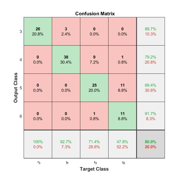
Discontinuous Galerkin (PolyDG) method [6, 1, 16, 3, 17], the Virtual Element
Method (VEM) [9, 10, 11, 7] and the hybrid high-order method [27, 24, 25, 26,
28]. This calls for the need to develop effective algorithms to handle polygonal
and polyhedral grids and to assess their quality (see e.g. [5]). Among the open
problems, there is the issue of handling polytopic mesh refinement [33, 30, 12],
i.e. partitioning mesh elements into smaller elements to produce a finer grid,
and agglomeration strategies [18, 2, 6], i.e. merging mesh elements to obtain
coarser grids. Indeed, during either refinement or agglomeration it is important
to preserve the quality of the underlying mesh, because this might affect the
overall performance of the method in terms of stability and accuracy.
In this work, we propose a new strategy to handle polygonal grid refinement
based on Convolutional Neural Networks (CNNs). CNNs are machine learning
algorithms that are particularly well suited for image classification when clearly
defined rules cannot be deduced. Indeed, they have been successfully applied
in many areas, especially computer vision [34]. In recent years there has been
a great development of machine learning algorithms to enhance and accelerate
numerical methods for scientific computing. Examples include, but are not lim-
ited to, [36, 35, 39, 38, 29, 37].
In this work we show that CNNs can be successfully employed to identify cor-
rectly the “shape” of a polygonal element without resorting to any geometric
property. This information can then be exploited to apply tailored refinement
strategies for different families of polygons. This approach has several advan-
tages:
   • It helps preserving the mesh quality, since it can be easily tailored for
     different types of elements.
   • It can be combined with suitable (user-defined) refinement strategies.
   • It is independent of the numerical method employed to discretize the un-
     derlying differential model.
   • The overall computational costs are kept low, since the training phase of a
     CNN is performed off line and it is independent of the differential problem
     at hand.
In this paper, we show that CNNs can be used effectively to boost either exist-
ing refinement criteria, such as the Mid-Point (MP) strategy, that consists in
connecting the edges midpoints of the polygon with its centroid, and we also
propose a refinement algorithm that employs pre-defined refinement rules on
regular polygons. We refer to these paradigms as CNN-enhanced refinement
strategies. To demonstrate the capabilities of the proposed approach we con-
sider a second-order model problem discretized by either PolyDG methods and
VEMs and we test the two CNN-enhanced refinement strategies based on poly-
gons’ shape recognition. For both the CNNs-enhanced refinement strategies we
demonstrate their effectiveness through an analysis of quality metrics and ac-
curacy of the discretization methods.

                                        2
Figure 1: Refinement strategies for triangular, quadrilateral, pentagonal and
hexagonal polygons. The vertices of the original polygon K are marked with
black dots.
The paper is organized as follows. In Section 2 we show how to classify poly-
gons’ shape using a CNN. In Section 3 we present new CNN-enhanced refine-
ment strategies and different metrics to measure the quality of the proposed
refinement strategies. In Section 4 we train a CNN for polygons classification.
In Section 5 we validate the new refinement strategies on a set of polygonal
meshes, whereas in Section 6 we test them when employed with PolyDG and
Virtual Element discretizations of a second-order elliptic problem. Finally in
Section 7 we draw some conclusions.
2 Polygon classification using CNNs
In this section we discuss the problem of correctly identify the “shape” of a
general polygon, in order to later apply a suitable refinement strategy accord-
ing to the chosen label of the classification. We start by observing that for
polygons with “regular” shapes, e.g. triangles, squares, pentagons, hexagons
and so on, we can define ad-hoc refinement strategies. For example, satisfactory
refinement strategies for triangular and quadrilateral elements can be designed
in two dimensions, as shown in Figure 1 (left). If the element K is a triangle,
the midpoint of each edge is connected to form four triangles; if K is a square,
the midpoint of each edge is connected with the centroid of the vertices of the
polygon (to which we will refer as “centroid”, for short), i.e. the arithmetical
average of the vertices coordinates, to form four squares. For a regular poly-
gon K with more than fours edges, suitable refinement strategies can also be
devised, see e.g. [33] and Figure 1 (right). The idea is to:
1. Construct a suitably scaled and rotated polygon K̂ with centroid that
coincide with the centroid of the initial polygon K.
2. Connect the vertices of K̂ with the midpoints of the edges K, forming a
pentagon for each vertex of the original polygon K.
This strategy induces a partition with as many elements as the number of ver-
tices of the original polygon K plus one. The above refinement strategies for
regular polygons have the following advantages:
• They produce regular structures, thus preserving mesh quality.
3Figure 2: Refinement
using Voronoi tessella-
tion. The vertices of the
original polygon K are
marked with full dots,
while seeds are marked
with empty dots.
• They enforce a modular structure, as the new elements have the same
structure of the original one, easing future refinements.
• They keep mesh complexity low, as they add few vertices and edges.
• They are simple to be applied and have a low computational cost.
The problem of refining a general polygonal element is still subject to ongoing
research. A possible strategy consist of dividing the polygon along a chosen
direction into two sub-elements [12]; this strategy is very simple and has an
affordable computational cost, and it also seems to be robust and to preserve
elements’ regularity. Because of its simplicity, however, this strategy can hardly
exploit particular structures of the initial polygon.
Another possibility is to use a Voronoi tessellation [30], where some points,
called seeds, are chosen inside the polygon K and each element of the new
partition is the set of points which are closer to a specific seed, as shown in
Figure 2. It is not obvious how many seeds to use and where to place them,
but the resulting mesh elements are fairly regular. The overall algorithm has a
consistent but reasonable computational cost.
Another choice is to use the Mid-Point (MP) strategy, which consist in con-
necting the midpoint of each edge of K with the centroid of K, as shown in
Figure 3 (top). This strategy is very simple and has a low computational cost.
Modularity is enforced, in the sense that the resulting elements of the mesh are
all quadrilaterals. However, nodes are added to adjacent elements, as shown in
Figure 4, unless suitable (geometric) checks are included. The main drawback
of this strategy is that it potentially disrupts mesh regularity and the number
of mesh elements increases very rapidly. Therefore, which refinement strategy is
the most effective depends on the problem at hand and the stability properties
of the numerical scheme used for its approximation.
In order to suitably drive these refinement criteria, we propose to use CNNs
to predict to which “class of equivalence” a given polygon belongs to. For ex-
ample in Figure 3 (top) we show two elements refined using the MP strategy.
They are clearly a quadrilateral and a pentagon, respectively, but their shapes
are very similar to a triangle and a square respectively, and hence they should
be refined as in Figure 3 (bottom). Loosely speaking, we are trying to access
4Figure 3: Top: the two polygons have been refined based on employing the
“plain” MP rules. Bottom: the two polygons have been first classified to belong
to the class of “triangular” and “quadrilateral” element, respectively, and then
refined accordingly. The vertices of the original polygons are marked with black
dots.
whether the shape of the given polygon is “more similar” to a triangle, or a
square, or a pentagon, and so on. The general algorithm is the following:
1. Let P = {P1 , P2 , ... Pm } be a set of possible polygons to be refined and
let R = {R1 , R2 , ... Rn } be a set of possible refinement strategies.
2. We build a classifier F : P → R in such a way that suitable mesh quality
metrics are preserved [5, 41] (quality metrics will be described later in
Section 3.3). The set of all polygons mapped into the same refinement
strategy is a “class of equivalence”.
In principle, any classifier F may be used. However, understating the specific
relevance of different geometric features of a general polygon (e.g. number
Figure 4: Left: the initial grid. Middle: the MP refinement strategy has been
applied to the square on the left, therefore adding one node to the adjacent
square on the right. Right: the MP refinement strategy has been applied also
to the square on the right, dividing it into five sub-elements. The vertices of the
grids that are employed to apply the MP refinement strategy of each stage are
marked with black dots.
5Figure 5: Illustrative examples of polygons belonging to the class of “squares”.
They have been obtained by adding small distortions or extra aligned vertices
to the reference square, plus rotations and scalings in some cases. The vertices
are marked with black dots.
Figure 6: Binary image of a pentagon of size 50×50 pixels. Each pixel has value
1 (white pixel) if it is inside the polygon and 0 otherwise (black pixel). The
binary images of each mesh element are then employed to classify the shape of
the element, avoiding the automatic and exclusive use of geometric information.
of edges, area, etc...) might not be enough to operate a suitable classification.
Instead, we can construct a database of polygons that can be used to “train” our
classifier F . In order to construct such database we proceed as follows. Starting
from the “reference” polygon in a class (e.g. the reference triangle for the class
“triangles”, the reference square for the class “squares” and so on) we generate a
set of perturbed elements that still belong to the same class and are obtained by
adding new vertices and/or adding noise to them, introducing rotations and so
on. An illustrative example in the case of the class “squares” is show in Figure 5.
Training a function with labelled data is known as “supervised learning”, and
CNNs are particularly well suited to deal with image classification problems in
this context. Indeed, because of the inherently “image classification” nature of
this problem, polygons can be easily converted into binary images: each pixel
assumes value 1 if it is inside the polygon and 0 otherwise, as shown in Figure 6.
2.1 Supervised learning for image classification
Consider a two dimensional gray-scale image, represented by a tensor B ∈
Rm×n , m, n ≥ 1, and the corresponding label vector y ∈ [0, 1]` , where ` ≥ 2
is the total number of classes, and [y]j is the probability of B to belong to the
class j for j = 1 : `. For the case of polygons classification B ∈ {0, 1}m×n ,
6i.e images are binary. Moreover, in our case the classes are given by the label
“triangle”, “square”, “pentagon” and so on.
In a supervised learning framework, we are given a dataset of desired input-
output couples {(Bi , yi )}N
i=1 , where N is number of labelled data. We consider
then an image classifier represented by a function of the from F : Rm×n → (0, 1)` ,
in our case a CNN, parameterized by w ∈ RM where M ≥ 1 is the number of
parameters. Our goal is to tune w so that F minimizes the data misfit, i.e.
X
min l(F (Bi ), yi ),
w∈RM
i∈I
where I is a subset of {1, 2, ..., N } and l is the cross-entropy loss function defined
as
X`
l(F (B), y) = −[y]j log[F (B)]j .
j=1
This optimization phase is also called “learning” or “training phase”. During
this phase, a known shortcoming is “overfitting”: the model fits very well the
data used in the training phase, but performs poorly on new data. For this
reason, the data set is usually splitted into: i) training set: used to tune the
parameters during the training phase; ii) validation set: used to monitor the
model capabilities on different data during the training phase. The training is
halted if the error on the validation set starts to increase; iii) test set: used to
access the actual model performance on new data after the training.
While the training phase can be computationally demanding, because of the
large amount of data and parameters to tune, it needs to be performed off line
once and for all. Instead, classifying a new image using a pre-trained model
is computationally fast: it requires only to evaluate F on a new input. The
predicted label is the one with the highest estimated probability.
2.2 CNNs
CNNs are parameterized functions, constructed by composition of simpler func-
tions called “layers of neurons”. A typical CNN architecture is as follows
CNN : Rm×n → (0, 1)` ,
CNN = Conv → Norm → ReLU → Pool →
Conv → Norm → ReLU → Pool →
...
Conv → Norm → ReLU → Linear → Softmax,
where Conv, Norm, ReLU, Pool, Linear and Softmax are suitable func-
tions that will be explained in the following, and the arrow notation is defined
as f → g := g ◦ f , being f and g two generic functions. We are now going to
define each of the above mentioned layers.
Convolutional layers are linear mappings of the form Conv : Rm×n×c → Rm×n×h̄
7with m, n, c, h̄ ≥ 1. Consider a two dimensional gray-scale image B ∈ Rm×n and
a kernel matrix K ∈ R(2k+1)×(2k+1) of coefficients to be tuned. We can define
the convolution operator [·]i,j as
k
X
[K ∗ B]i,j = [K]k+1+p,k+1+q [B]i+p,j+q , i = 1 : m, j = 1 : n,
p,q=−k
with zero padding, i.e. Bi+p,j+q = 0 when indexes are out of range. This
operation can be viewed as a filter scanning through the image B, extracting
local features that depend only on small subregions of the image. This is effective
because a key property of images is that close pixels are more strongly correlated
than distant ones. The scanning filter mechanism provides the basis for the
invariance of the output to translations and distortions of the input image [13],
which is fundamental in our setting. Consider now an image with c channels
B ∈ Rm×n×c , e.g. in the input layer c = 1 for gray-scale images and c = 3
for color images, on which we want to apply h̄ different feature maps. This
corresponds to applying a convolutional layer of the form
c
X
[Conv(B)]i = [K]:,:,i,j ∗ [B]:,:,j + [b]i 1, i = 1 : h̄,
j=1
where the colon index denotes that all the indexes along that dimension are
considered, 1 ∈ Rm×n is the m × n matrix with all entries equal to 1, K ∈
R(2k+1)×(2k+1)×h̄×c is a kernel matrix and b ∈ Rh̄ is a bias vector of coefficients
to be tuned.
Non-linearity is introduced using the so-called “activation functions”. A popular
choice is the rectified linear unit ReLU(x) = max(0, x), with x ∈ R. It is applied
element-wise to the output of the previous layer.
Pooling layers are used to perform down-sampling, such as the max pooling
layer that computes the maximum of the input region-wise Pool : Rm×n →
m n
Rd s e×d s e ,
[Pool(B)]i,j = max Bs(i−1)+p,s(j−1)+q ,
p,q=1:k
with s ≥ 1 and zero padding. They are applied to each channel of the input
image. We point out that these layers enforce the invariance of the output with
respect to translations of the input.
In practise, subsequent application of convolutional, activation and pooling lay-
ers may be used to obtain a larger degree of invariance to input transformations
such as rotations, distortions, etc. Then, image features are linearly separated
using a dense layer of the form Linear : Rn → R` ,
Linear(x) = W x + b,
where n ≥ 1 is number of outputs of the previous layer, ` is the total number
of output labels, W ∈ R`×n and b ∈ R` are coefficients to be tuned.
8Figure 7: Simplified scheme of a CNN architecture employed for classification of
the shape of polygons. The little squares applied in every layer represent filters
scanning through the images.
The last layer needs to map the function output into (0, 1)` . A common choice
is the softmax function Softmax : R` → R` ,
exi
[Softmax(x)]i = P` .
j=1 exj
Additionally, batch normalization layers maybe used to speed up training and
reduce the sensitivity to network initialization [32]. A batch normalization ma-
2
nipulates its inputs xi by first calculating the mean µB and variance σB over
a mini-batch and over each input channel. Then, it calculates the normalized
activations as
xi − µB
x̂i = p 2 .
σB +
Here, improves numerical stability when the mini-batch variance is very small.
To allow for the possibility that inputs with zero mean and unit variance are
not optimal for the layer that follows the batch normalization layer, the batch
normalization layer further shifts and scales the activations as yi = Norm(xi ) =
γ x̂i + β. Here, the offset β and scale factor γ are learnable parameters that are
updated during network training, respectively. These layers can be applied
before the activation functions.
A visual representation of a CNN is shown in Figure 7 for the case of regular
polygons classification.
9L = 3 (triangle) L = 4 (quad) L = 5 (pentagon) L = 6 (hexagon)
Figure 8: Samples of polygons refined using the MP (top), CNN-MP (middle)
and CNN-RP (bottom) refinement strategies. The elements have been classified
using the CNN algorithm with labels L = 3, 4, 5, 6, respectively. The vertices of
the original polygons are marked with black dots.
3 CNN-enhanced refinement strategies
In this section we present two strategies to refine a general polygon that exploit a
pre-classification step of the polygon shape. More specifically, we assume that a
CNN for automatic classification of the polygon label is given. The first strategy
consists in enhancing the classical MP algorithm, whereas the second strategy
exploits the refinement criteria for regular polygons illustrated in Section 2.
3.1 A CNN-enhanced MP strategy
Assume we are given a general polygon P to be refined and its label L, obtained
using a CNN for classification of polygon shapes. Here L ≥ 3 is an integer,
where L = 3 corresponds to the label “triangle”, L = 4 corresponds to the label
“square”, and so on. If the polygon P has a large number of (possibly aligned)
vertices, applying the MP strategy may lead to a rapid deterioration of the shape
regularity of the refined elements. In order to reduce the number of elements
produced via refinement and to improve their quality, a possible strategy is to
enhance via CNNs the MP refinement strategy, and apply the MP refinement
strategy not to the original polygon P but to a suitable approximate polygon
P̂ with a number of vertices L identified by the CNN classification algorithm,
as described in Algorithms 1 and 2. Examples of refined polygons using the
MP strategy are shown in Figure 8 (top) whereas the analogous ones obtained
employing the CNN-enhanced Mid-Point (CNN-MP) refinement strategy are
10Algorithm 1: CNN-enhanced Mid-Point (CNN-MP) refinement strat-
egy
Input: polygon P .
Output: partition of P into polygonal sub-elements.
1 Convert P , after a proper scaling, to a binary image as shown in
Figure 6.
2 Apply a CNN for classification of the polygon shape and obtain its
label L ≥ 3.
3 Based on L, identify the refinement points on the boundary of P , as
described in Algorithm 2.
4 Connect the refinement points of P to its centroid cP .
Algorithm 2: Identification of the refinement points
Input: polygon P , label L ≥ 3.
Output: refinement points on the boundary of P .
1 Build a polygon P̂ suitably approximating P : select L vertices
PL
v̂1 , v̂2 , ...v̂L , among the vertices of P , that maximize i,j=1 ||v̂i − v̂j ||.
2 Compute the centroid cP of P , the edge midpoints of P and the edge
midpoints {m̂i }L i=1 of P̂ .
3 For every edge midpoint m̂i of P̂ : find the closest point to m̂i and cP ,
among the vertices and the edges midpoints of P .
shown in Figure 8 (middle). We point out that the computational cost of the
CNN-MP strategy is very low. Moreover, parallelism is enforced in a stronger
sense: the CNN does not distinguish between one edge of a polygon and two
aligned edges, solving the problem of refining adjacent elements pointed out in
Figure 4.
3.2 A new “reference-polygon” refinement strategy
Assume, as before, that we are given a general polygon P to be refined together
with its label L ≥ 3, that can be obtained employing a CNN classification al-
gorithm. If the given polygon is a reference polygon we could refine it based
on employing the refinement strategies described in Section 2 and illustrated
in Figure 1, where the cases L = 3, 4, 5, 6 are reported. Our goal is to extend
these strategies so that they can be applied to general polygons. In order to
do that, the idea of the algorithm is to first compute the refinement points of
P , as before, and then connect them using the refinement strategy for the class
L. More precisely, our new CNN-enhanced Reference Polygon (CNN-RP) re-
finement strategy is described in Algorithms 2 and 3 and illustrated in Figure 8
(bottom). Notice that lines 1-2-3 in Algorithm 3 are the same as in Algorithm
11Algorithm 3: CNN-enhanced Reference Polygon (CNN-RP) refine-
ment strategy
Input: polygon P .
Output: partition of P into polygonal sub-elements.
1 Convert P , after a proper scaling, to a binary image as shown in
Figure 6.
2 Apply a CNN for classification of the polygon shape and obtain its
label L ≥ 3.
3 Based on L, identify the refinement points on the boundary of P , as
described in Algorithm 2.
4 if L = 3 then
5 Connect the refinement points of P so as to form triangular
sub-elements.
6 end
7 if L = 4 then
8 Connect the refinement points of P to its centroid, so as to form
quadrilateral sub-elements.
9 end
10 if L ≥ 5 then
11 Construct inside of P a suitably scaled and rotated regular polygon
with L vertices and with the same centroid of P .
12 Connect the vertices of the inner regular polygon with the
refinement points of the outer polygon P , so as to form
sub-elements as shown in Figure 1.
13 end
1. This strategy can be applied off line with a low computational cost and has
the advantage to enforce parallelism as each mesh element can be refined inde-
pendently.
Notice that for a non-convex polygon, the CNN-RP and the CNN-MP strate-
gies do not guarantee in general to generate a valid refined element, because the
centroid could lie outside the polygon. In practise, they work well even if the
polygon is “slightly” non-convex. However, in case of a non-valid refinement, it
is always possible to first subdivide the polygon into two elements, possibly of
comparable size, by connecting two of its vertices.
3.3 Quality metrics
In order to evaluate the quality of the proposed refinement strategies, we recall
some of the quality metrics introduced in [5]. The diameter of a domain D is
defined, as usual, as diam(D) := sup{|x − y|, x, y ∈ D}. Given a polygonal
12Figure 9: A polygon with
a small edge. Although its
shape is regular, ER and
NPD metrics assume small
values, depending on the
size of the smallest edge.
mesh, i.e. a set of non-overlapping polygonal regions {Pi }N
i=1 , NP ≥ 1, that
P
covers a domain Ω, we can define the mesh size h = maxi=1:NP diam(Pi ). For
a mesh element Pi , the Uniformity Factor (UF) is defined as UFi = diam(P
h
i)
,
i = 1, ..., NP . This metric takes values in [0, 1].
For a polygon P , we also introduce the following quality metrics, taken from
[5]:
diam(P )
1. Uniformity Factor (UF): h .
2. Circle Ratio (CR): ratio between the radius of the inscribed circle and the
radius of the circumscribed circle of P :
max{B(r)⊂P } r
,
diam(P )/2
where B(r) is a ball of radius r.
3. Area-Perimeter Ratio (APR):
4π area(P )
.
perimeter(P )2
4. Minmum Angle (MA): minimum inner angle of P , normalized by 180◦ .
5. Edge Ratio (ER): ratio between the shortest and the longest edge of P .
6. Normalized Point Distance (NPD): minimum distance between any two
vertices of P , divided by the diameter of the circumscribed circle of P .
These metrics are scale-independent and take values in [0, 1]. The more regular
the polygons are, the larger CR, APR and MA are. Large values of ER and NPD
also indicate that the polygon is well proportioned and not skewed. However,
small values of ER and NPD do not necessarily mean that the element is not
shaped-regular, as shown in Figure 9.
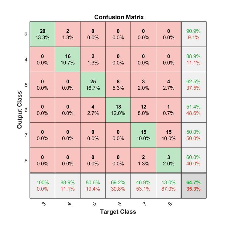
13Figure 10: Confusion matrices for polygons classification. Left: the number of
classes is ` = 6 and the target classes vary from L = 3 (triangles) to L = 8
(octagons). Right: the number of classes is ` = 4 and the target classes vary
from L = 3 (triangles) to L = 6 (hexagons). The prediction accuracy for each
target class decreases as more target classes are considered.
4 CNN training
The CNN architecture we used for polygons classification is given by
CNN : {0, 1}50×50 → (0, 1)` , where
CNN = Conv(k = 1, h̄ = 8) → Norm → ReLU → Pool(k = 2, s = 2) →
Conv(k = 1, h̄ = 16) → Norm → ReLU → Pool(k = 2, s = 2) →
Conv(k = 1, h̄ = 32) → Norm → ReLU → Linear → Softmax,
where k, h̄, s are defined as in Section 2.2. For each class, we generated 125
images transforming regular polygons by adding edges and noise to the vertices.
Scaling and rotations are added randomly every time an image is selected, since
the same image is selected multiple times during training. We set training, val-
idation and test sets equal to 60%-20%-20% of the whole dataset, respectively.
Initially we selected the number of target classes to be equal to ` = 6, i.e. poly-
gons are sampled from triangles to octagons. We show the confusion matrix in
Figure 10 (left). The same results obtained with ` = 6, i.e. target classes vary-
ing from L = 3 (triangles) to L = 6 (hexagons), are shown in Figure 10 (right).
From these results it seems that the prediction accuracy is better in the case of a
14smaller set of target classes. This is expected, as for example a regular octagon
is much more similar, in terms of angles amplitude and edges length, to a regular
heptagon than to a regular triangle. Moreover, for polygons with many edges
more pixels might be required in order to appreciate the differences between
them. In the following numerical experiments we have decided to choose ` = 4,
as this choice seems to balance the effectiveness of our classification algorithm
with the computational cost. We also remark that for the following reasons:
• Refining heptagons and octagons as if they were hexagons does not seem
to affect dramatically the quality of the refinement.
• Ad-hoc refinement strategies for polygons with many edges seem to be
less effective because more sub-elements are produced.
• A considerable additional computational effort might be required to in-
clude more classes.
• The more classes we use, the easier the possibility of a misclassification
error is and hence to end up with a less robust refinement procedure.
Considering polygon classes ranging from triangles to hexagons yields a satisfac-
tory accuracy of 80% as shown in Figure 10 (right). Thanks to the limited num-
ber of dataset samples and network parameters, the whole algorithm (dataset
generation, CNN training and testing) took approximately one minute using
MATLAB2019b on a Windows OS 10 Pro 64-bit, Intel(R) Core(TM) i7-8750H
CPU (2.20GHz / 2.21GHz) and 16 GB RAM memory. Again, notice that the
performance could be improved by considering more data and using an archi-
tecture with more layers. We also point out that our goal is not to optimize
this process, but rather to show the importance of a classification step in the
refinement procedure, and how CNNs can be employed for this purpose.
5 Validation on a set of polygonal meshes
In this section we compare the performance of the proposed algorithms. We
consider four different coarse grids of the domain (0, 1)2 : a grid of triangles, a
Voronoi grid, a smoothed Voronoi grid obtained with Polymesher [42], and a
grid made of non-convex elements. In Figure 11 these grids have been succes-
sively refined uniformly, i.e. each mesh element has been refined, for three times
using the MP, the CNN-MP and the CNN-RP strategies. The final number of
mesh elements is shown in Table 1. We observe that on average the MP strategy
produced 4 times more elements than the CNN-RP strategy, and 6 times more
than CNN-MP strategy.
In Figures 12 we show the computed quality metrics described in Section 3.3
on the grids of Figure 11 (triangles, Voronoi, smoothed Voronoi, non-convex).
Despite the fact that the performance are considerably grid dependent, the
15# mesh elements triangles Voronoi smoothed Voronoi non-convex
initial grid 32 9 10 14
MP 6371 2719 3328 4502
CNN-RP 2048 578 784 1030
CNN-MP 1146 391 666 682
Table 1: Final number of elements for each mesh shown in Figure 11: a grid
of triangles, a Voronoi grid, a smoothed Voronoi grid and a grid made of non-
convex elements have been uniformly refined using the Midp-Point (MP), the
CNN-enhanced Mid-Point (CNN-MP) and the CNN-enhanced Reference Poly-
gon (CNN-RP) strategies. On average, the MP strategy produced 4 times more
elements than the CNN-RP strategy, and 6 times more elements than CNN-MP
strategy.
CNN-RP strategy and the CNN-MP strategy seem to perform in a comparable
way. Moreover, the CNN-RP and the CNN-MP strategies perform consistently
better than the MP strategy, since their distributions are generally more con-
centrated toward the value 1.
6 Testing CNN-based refinement strategies with
PolyDG and Virtual Elements discretizations
In this section we test the effectiveness of the proposed refinement strategies,
to be used in combination with polygonal finite element discretizations. To this
aim we consider PolyDG and Virtual Element discretizations of the following
model problem: find u ∈ H01 (Ω) such that
Z Z
∇u · ∇v = f v ∀v ∈ H01 (Ω), (1)
Ω Ω
2
with f ∈ L (Ω) a given forcing term. The workflow is as follows:
1. Generate a grid for Ω.
2. Compute numerically the solution of problem (1) using either the VEM
[9, 10, 11, 7] or the PolyDG method [6, 1, 16, 3, 17].
3. Compute the error. In the VEM case the error is measured using the H01
norm (see [10] and [40], for details), while in the PolyDG case the error is
computed using the DG norm (see [4, 23], for details)
X X
kvk2DG = k∇vk2L2 (P ) + kγ 1/2 JvKk2L2 (F ) ,
P F
where γ is the stabilization function (that depends on the discretization
parameters and is chosen as in [16]), P is a polygonal mesh element and
F is an element face. The jump operator J·K is defined as in [4].
16initial grid MP CNN-RP CNN-MP
triangles
Voronoi
smoothed Voronoi
non-convex
Figure 11: In the first column, coarse grids of the domain Ω = (0, 1)2 : a grid of triangles, a
Voronoi grid, a smoothed Voronoi grid, and a grid made of non-convex elements. Second to fourth
columns: refined grids obtained after three steps of uniform refinement based on employing the MP
(second column), the CNN-RP (third column) and the CNN-MP (fourth column) strategies. Each
row corresponds to the same initial grid, while each column corresponds to the same refinement
strategy.
17triangles Voronoi smoothed Voronoi non-convex
MP CNN-RP CNN-MP MP CNN-RP CNN-MP MP CNN-RP CNN-MP MP CNN-RP CNN-MP
40 %
Uniformity Factor
20 %
40 % 20 % 30 % 15 %
grid elements
grid elements
grid elements
grid elements
20 % 10 %
20 % 10 %
10 % 5%
0% 0% 0% 0%
0 0.2 0.4 0.6 0.8 1 0 0.2 0.4 0.6 0.8 1 0 0.2 0.4 0.6 0.8 1 0 0.2 0.4 0.6 0.8 1
MP CNN-RP CNN-MP MP CNN-RP CNN-MP MP CNN-RP CNN-MP MP CNN-RP CNN-MP
30 %
30 % 20 %
Circle Ratio
40 %
20 % 15 %
grid elements
grid elements
grid elements
grid elements
20 %
10 %
20 % 10 % 10 %
5%
0% 0% 0% 0%
0 0.2 0.4 0.6 0.8 1 0 0.2 0.4 0.6 0.8 1 0 0.2 0.4 0.6 0.8 1 0 0.2 0.4 0.6 0.8 1
Area-Perimeter Ratio
MP CNN-RP CNN-MP MP CNN-RP CNN-MP MP CNN-RP CNN-MP 40 % MP CNN-RP CNN-MP
60 % 40 %
80 %
30 %
30 % 60 %
grid elements
grid elements
grid elements
grid elements
40 %
20 %
20 % 40 %
20 %
10 % 10 %
20 %
0% 0% 0% 0%
0 0.2 0.4 0.6 0.8 1 0 0.2 0.4 0.6 0.8 1 0 0.2 0.4 0.6 0.8 1 0 0.2 0.4 0.6 0.8 1
MP CNN-RP CNN-MP MP CNN-RP CNN-MP MP CNN-RP CNN-MP MP CNN-RP CNN-MP
60 % 30 % 30 %
Minimum Angle
60 %
grid elements
grid elements
grid elements
grid elements
40 % 20 % 20 %
40 %
20 % 10 % 20 % 10 %
0% 0% 0% 0%
0 0.2 0.4 0.6 0.8 1 0 0.2 0.4 0.6 0.8 1 0 0.2 0.4 0.6 0.8 1 0 0.2 0.4 0.6 0.8 1
MP CNN-RP CNN-MP MP CNN-RP CNN-MP MP CNN-RP CNN-MP 15 % MP CNN-RP CNN-MP
25 %
15 %
30 %
20 %
Edge Ratio
10 %
grid elements
grid elements
grid elements
grid elements
10 % 15 %
20 %
10 %
5%
10 % 5%
5%
0% 0% 0% 0%
0 0.2 0.4 0.6 0.8 1 0 0.2 0.4 0.6 0.8 1 0 0.2 0.4 0.6 0.8 1 0 0.2 0.4 0.6 0.8 1
Normalized Point Distance
MP CNN-RP CNN-MP 25 % MP CNN-RP CNN-MP MP CNN-RP CNN-MP MP CNN-RP CNN-MP
40 % 30 %
20 %
20 %
30 %
15 %
20 %
grid elements
grid elements
grid elements
grid elements
15 %
20 %
10 %
10 %
10 %
10 % 5%
5%
0% 0% 0% 0%
0 0.2 0.4 0.6 0.8 1 0 0.2 0.4 0.6 0.8 1 0 0.2 0.4 0.6 0.8 1 0 0.2 0.4 0.6 0.8 1
Figure 12: Computed quality metrics (Uniformity Factor, Circle Ratio, Minimum Angle, Edge
Ratio and Normalized Point Distance) for the refined grids reported in Figure 11 (second to fourth
column) and obtained based on employing different refinement strategies (MP, CNN-MP, CNN-RP).
184. Use the fixed fraction refinement strategy to refine a fraction r of the
number of elements. To refine the marked elements we employ one of the
proposed strategies. Here, in order to investigate the effect of the proposed
refinement strategies, we did not employ any a posteriori estimator of the
error, but we computed element-wise the local error based on employing
the exact solution.
6.1 Uniformly refined grids
When r = 1, the grid is refined uniformly, i.e. at each step each mesh element
is refined. The forcing term f in (1) is selected in such a way that the exact
solution is given by
u(x, y) = sin(πx) sin(πy).
The grids obtained after three steps of uniform refinement are those already re-
ported in Figure 11. In Figure 13 we show the computed errors as a function of
the number of degrees of freedom. We observe that the CNN-enhanced strate-
gies (both MP and RP ones) outperform the plain MP rule. The difference is
more evident for VEMs than for PolyDG approximations.
6.2 Adaptively refined grids
In this case we selected r = 0.3. The forcing term f in (1) is selected in such a
way that the exact solution is
u(x, y) = (1 − e−10x )(x − 1) sin(πy),
that exhibits a boundary layer along x = 0. Figure 14 shows the computed
grids after three steps of refinement for the PolyDG case. Very similar grids
have been obtained with Virtual Element discretizations.
In Figure 15 we show the computed errors as a function of the number of degrees
of freedom for both Virtual Element and PolyDG discretizations. The CNN-
enhanced strategies (both MP and RP ones) outperform the plain MP rule. The
difference is more evident for VEMs than for PolyDG approximations.
7 Conclusions
In this work, we successfully employed CNNs to enhance both existing refine-
ment criteria and new refinement procedures, withing polygonal finite element
discretizations of partial differential equations. In particular, we introduced two
refinement strategies for polygonal elements, named “CNN-RP strategy” and
“CNN-MP strategy”. The former proposes ad-hoc refinement strategies based
on reference polygons, while the latter is an improved version of the known MP
strategy. These strategies exploit a CNN to suitably classify polygons in order
19VEM PolyDG
0
10
−1/2
−1/2
Triangles grid
10−1
10−2
MP 10−1 MP
CNN-RP CNN-RP
CNN-MP CNN-MP
10−3
102 103 104 102 103 104
Degrees of freedom Degrees of freedom
10−0.5 −1/2 100 −1/2
Voronoi grid
10−1
10−1.5 MP MP
CNN-RP CNN-RP
CNN-MP CNN-MP
10−1
101 102 103 102 103 104
Degrees of freedom Degrees of freedom
Smoothed Voronoi grid
−1/2 −1/2
100
−1
10
10−2
MP MP
CNN-RP 10−1 CNN-RP
CNN-MP CNN-MP
102 103 104 101 102 103 104
Degrees of freedom Degrees of freedom
Non-convex grid
−1/2 100 −1/2
10−1
MP MP
CNN-RP CNN-RP
CNN-MP CNN-MP
10−1
10−2
102 103 104 101 102 103 104
Degrees of freedom Degrees of freedom
Figure 13: Test case of Section 6.1. Computed errors as a function of the number
of degrees of freedom. Each row corresponds to the same initial grid (triangles,
Voronoi, smoothed Voronoi, non-convex) refined uniformly with the proposed
refinement strategies (MP, CNN-RP and CNN-MP), while each column corre-
sponds to a different numerical method (VEM left and PolyDG right).
20initial grid MP CNN-RP CNN-MP
triangles
Voronoi
smoothed Voronoi
non-convex
Figure 14: Adaptively refined grids for the test case of Section 6.2. Each row corresponds to the same
initial grid (triangles, Voronoi, smoothed Voronoi, non-convex), while the second-fourth columns
correspond to the different refinement strategies (MP, CNN-RP, CNN-MP). Three successively
adaptive refinement steps have been performed, with a fixed fraction refinement criterion (refinement
fraction r set equal to 30%).
21VEM PolyDG
100.2
10−0.8 −1/2 −1/2
Triangles grid
100
10−1
10−0.2
10−1.2 10−0.4
MP MP
CNN-RP CNN-RP
−0.6
CNN-MP 10 CNN-MP
10−1.4
102 103 102 102.5 103 103.5
Degrees of freedom Degrees of freedom
10−0.5 −1/2
100 −1/2
Voronoi grid
10−0.2
10−1
10−0.4
MP MP
10−0.6
10−1.5 CNN-RP CNN-RP
CNN-MP CNN-MP
10−0.8 2
102 103 10 102.5 103 103.5
Degrees of freedom Degrees of freedom
100.2
Smoothed Voronoi grid
−1/2
100 −1/2
10−1
10−0.2
10−0.4
10−1.5 MP MP
10−0.6
CNN-RP CNN-RP
CNN-MP CNN-MP
10−0.8
102 103 102 103
Degrees of freedom Degrees of freedom
−1/2 100
Non-convex grid
10−1 −1/2
10−0.2
10−0.4
10−0.6
MP MP
CNN-RP CNN-RP
CNN-MP 10−0.8 CNN-MP
10−2
102.5 103 103.5 103 104
Degrees of freedom Degrees of freedom
Figure 15: Test case of Section 6.2. Computed errors as a function of the number
of degrees of freedom. Each row corresponds to the same initial grid (triangles,
Voronoi, smoothed Voronoi, non-convex) refined adaptively with a fixed frac-
tion refinement criterion (refinement fraction r set equal to 30%) with different
strategies (MP, CNN-RP and CNN-MP), while each column corresponds to a
different numerical method (VEM left and PolyDG right).
22to later apply an ad-hoc refinement strategy. This approach has the advantage
to be made of interchangeable pieces: any algorithm can be employed to classify
mesh elements, as well as any refinement strategy can be employed to refine a
polygon with a given label.
We have shown that correctly classifying elements’ shape based on employing
CNNs can improve consistently and significantly the quality of the grids and the
accuracy of polygonal finite element methods employed for the discretization.
Specifically, this has been measured in terms of less elements produced on aver-
age at each refinement step, in terms of improved quality of the mesh elements
according to different quality metrics, and in terms of improved accuracy using
numerical methods such as PolyDG methods and VEMs. These results show
that classifying correctly the shape of a polygonal element plays a key role in
which refinement strategy to choose, allowing to extend and to boost existing
strategies. Moreover, this classification step has a very limited computational
cost when using a pre-trained CNN. The latter can be made off line once and
for all, independently of the model problem under consideration.
In terms of future research lines, we plan to extend these algorithms to three
dimensional polyhedral grids. The CNN architecture is naturally designed to
handle three dimensional images, while the design of effective refinement strate-
gies in three dimensions is under investigation.
References
[1] P. F. Antonietti, S. Giani, and P. Houston. “hp-version composite discon-
tinuous Galerkin methods for elliptic problems on complicated domains”.
In: SIAM Journal on Scientific Computing 35.3 (2013), A1417–A1439.
[2] P. F. Antonietti et al. “An agglomeration-based massively parallel non-
overlapping additive Schwarz preconditioner for high-order discontinuous
Galerkin methods on polytopic grids”. In: Mathematics of Computation
(2020).
[3] P. F. Antonietti et al. “Review of discontinuous Galerkin finite element
methods for partial differential equations on complicated domains”. In:
Building bridges: connections and challenges in modern approaches to nu-
merical partial differential equations. Springer, 2016, pp. 281–310.
[4] D. N. Arnold et al. “Unified analysis of discontinuous Galerkin methods for
elliptic problems”. In: SIAM Journal on Numerical Analysis 39.5 (2002),
pp. 1749–1779.
[5] M. Attene et al. “Benchmark of Polygon Quality Metrics for Polytopal
Element Methods”. In: arXiv preprint arXiv:1906.01627 (2019).
[6] F. Bassi et al. “On the flexibility of agglomeration based physical space dis-
continuous Galerkin discretizations”. In: Journal of Computational Physics
231.1 (2012), pp. 45–65.
23[7] L. Beirao da Veiga et al. “Mixed virtual element methods for general
second order elliptic problems on polygonal meshes”. In: ESAIM: Mathe-
matical Modelling and Numerical Analysis 50.3 (2016), pp. 727–747.
[8] L. Beirao da Veiga, K. Lipnikov, and G. Manzini. The mimetic finite
difference method for elliptic problems. Vol. 11. Springer, 2014.
[9] L. Beirão da Veiga et al. “Basic principles of virtual element methods”.
In: Mathematical Models and Methods in Applied Sciences 23.01 (2013),
pp. 199–214.
[10] L. Beirão da Veiga et al. “The hitchhiker’s guide to the virtual element
method”. In: Mathematical models and methods in applied sciences 24.08
(2014), pp. 1541–1573.
[11] L. Beirão da Veiga et al. “Virtual element method for general second-
order elliptic problems on polygonal meshes”. In: Mathematical Models
and Methods in Applied Sciences 26.04 (2016), pp. 729–750.
[12] S. Berrone, A. Borio, and A. D’Auria. “Refinement strategies for polygonal
meshes applied to adaptive VEM discretization”. In: Finite Elements in
Analysis and Design 186 (2021), p. 103502.
[13] C. M. Bishop. Pattern recognition and machine learning. springer, 2006.
[14] F. Brezzi, K. Lipnikov, and M. Shashkov. “Convergence of the mimetic
finite difference method for diffusion problems on polyhedral meshes”. In:
SIAM Journal on Numerical Analysis 43.5 (2005), pp. 1872–1896.
[15] F. Brezzi, K. Lipnikov, and V. Simoncini. “A family of mimetic finite dif-
ference methods on polygonal and polyhedral meshes”. In: Mathematical
Models and Methods in Applied Sciences 15.10 (2005), pp. 1533–1551.
[16] A. Cangiani, E. H. Georgoulis, and P. Houston. “hp-version discontinuous
Galerkin methods on polygonal and polyhedral meshes”. In: Mathematical
Models and Methods in Applied Sciences 24.10 (2014), pp. 2009–2041.
[17] A. Cangiani et al. hp-Version discontinuous Galerkin methods on polygonal
and polyhedral meshes. Springer, 2017.
[18] T. F. Chan, J. Xu, and L. Zikatanov. “An agglomeration multigrid method
for unstructured grids”. In: Contemporary Mathematics 218 (1998), pp. 67–
81.
[19] B. Cockburn, B. Dong, and J. Guzmán. “A superconvergent LDG-hybridizable
Galerkin method for second-order elliptic problems”. In: Mathematics of
Computation 77.264 (2008), pp. 1887–1916.
[20] B. Cockburn, J. Gopalakrishnan, and R. Lazarov. “Unified hybridization
of discontinuous Galerkin, mixed, and continuous Galerkin methods for
second order elliptic problems”. In: SIAM Journal on Numerical Analysis
47.2 (2009), pp. 1319–1365.
[21] B. Cockburn, J. Gopalakrishnan, and F.-J. Sayas. “A projection-based
error analysis of HDG methods”. In: Mathematics of Computation 79.271
(2010), pp. 1351–1367.
24[22] B. Cockburn, J. Guzmán, and H. Wang. “Superconvergent discontinuous
Galerkin methods for second-order elliptic problems”. In: Mathematics of
Computation 78.265 (2009), pp. 1–24.
[23] B. Cockburn, G. E. Karniadakis, and C.-W. Shu. Discontinuous Galerkin
methods: theory, computation and applications. Vol. 11. Springer Science
& Business Media, 2012.
[24] D. A. Di Pietro and A. Ern. “A hybrid high-order locking-free method
for linear elasticity on general meshes”. In: Computer Methods in Applied
Mechanics and Engineering 283 (2015), pp. 1–21.
[25] D. A. Di Pietro and A. Ern. “Hybrid high-order methods for variable-
diffusion problems on general meshes”. In: Comptes Rendus Mathématique
353.1 (2015), pp. 31–34.
[26] D. A. Di Pietro, A. Ern, and S. Lemaire. “A review of hybrid high-order
methods: formulations, computational aspects, comparison with other meth-
ods”. In: Building bridges: connections and challenges in modern approaches
to numerical partial differential equations. Springer, 2016, pp. 205–236.
[27] D. A. Di Pietro, A. Ern, and S. Lemaire. “An arbitrary-order and compact-
stencil discretization of diffusion on general meshes based on local recon-
struction operators”. In: Computational Methods in Applied Mathematics
14.4 (2014), pp. 461–472.
[28] D. A. Di Pietro and J. Droniou. The Hybrid High-Order method for poly-
topal meshes. Vol. 19. Springer, 2019.
[29] J. S. Hesthaven and S. Ubbiali. “Non-intrusive reduced order modeling of
nonlinear problems using neural networks”. In: Journal of Computational
Physics 363 (2018), pp. 55–78.
[30] T. Y. Hoshina, I. F. Menezes, and A. Pereira. “A simple adaptive mesh
refinement scheme for topology optimization using polygonal meshes”. In:
Journal of the Brazilian Society of Mechanical Sciences and Engineering
40.7 (2018), p. 348.
[31] J. Hyman, M. Shashkov, and S. Steinberg. “The numerical solution of
diffusion problems in strongly heterogeneous non-isotropic materials”. In:
Journal of Computational Physics 132.1 (1997), pp. 130–148.
[32] S. Ioffe and C. Szegedy. “Batch normalization: Accelerating deep network
training by reducing internal covariate shift”. In: International conference
on machine learning. PMLR. 2015, pp. 448–456.
[33] M.-J. Lai and G. Slavov. “On recursive refinement of convex polygons”.
In: Computer Aided Geometric Design 45 (2016), pp. 83–90.
[34] Y. LeCun, Y. Bengio, and G. Hinton. “Deep learning”. In: nature 521.7553
(2015), pp. 436–444.
[35] M. Raissi and G. E. Karniadakis. “Hidden physics models: Machine learn-
ing of nonlinear partial differential equations”. In: Journal of Computa-
tional Physics 357 (2018), pp. 125–141.
25[36] M. Raissi, P. Perdikaris, and G. E. Karniadakis. “Physics-informed neu-
ral networks: A deep learning framework for solving forward and inverse
problems involving nonlinear partial differential equations”. In: Journal
of Computational Physics 378 (2019), pp. 686–707.
[37] D. Ray and J. S. Hesthaven. “An artificial neural network as a troubled-
cell indicator”. In: Journal of Computational Physics 367 (2018), pp. 166–
191.
[38] F. Regazzoni, L. Dedè, and A. Quarteroni. “Machine learning of multi-
scale active force generation models for the efficient simulation of cardiac
electromechanics”. In: Computer Methods in Applied Mechanics and En-
gineering 370 (2020), p. 113268.
[39] F. Regazzoni, L. Dedè, and A. Quarteroni. “Machine learning for fast and
reliable solution of time-dependent differential equations”. In: Journal of
Computational Physics 397 (2019), p. 108852.
[40] S. Salsa. Partial differential equations in action: from modelling to theory.
Vol. 99. Springer, 2016.
[41] T. Sorgente et al. “The role of mesh quality and mesh quality indica-
tors in the Virtual Element Method”. In: arXiv preprint arXiv:2102.04138
(2021).
[42] C. Talischi et al. “PolyMesher: a general-purpose mesh generator for polyg-
onal elements written in Matlab”. In: Structural and Multidisciplinary
Optimization 45.3 (2012), pp. 309–328.
26You can also read