Evolution of Hard X-ray Sources and Ultraviolet Solar Flare Ribbons for a Confined Eruption of a Magnetic Flux Rope
←
→
Page content transcription
If your browser does not render page correctly, please read the page content below

Evolution of Hard X-ray Sources and Ultraviolet Solar Flare
          Ribbons for a Confined Eruption of a Magnetic Flux Rope
        Y. Guo (郭洋)1,2, M. D. Ding (丁明德)1,2, B. Schmieder3 , P. Démoulin3 , H. Li (黎辉)4
              1
                  Department of Astronomy, Nanjing University, Nanjing 210093, China

                                         guoyang@nju.edu.cn
2
        Key Laboratory for Modern Astronomy and Astrophysics (Nanjing University), Ministry
                               of Education, Nanjing 210093, China
    3
        LESIA, Observatoire de Paris, CNRS, UPMC, Université Paris Diderot, 5 place Jules
                                Janssen, 92190 Meudon, France
    4
         Purple Mountain Observatory, Chinese Academy of Sciences, Nanjing 210008, China

                                             ABSTRACT

               We study the magnetic field structures of hard X-ray sources and flare ribbons
           of the M1.1 flare in active region NOAA 10767 on 2005 May 27. We have found in
           a nonlinear force-free field extrapolation, over the same polarity inversion line, a
           small pre-eruptive magnetic flux rope located next to sheared magnetic arcades.
           Ramaty High Energy Solar Spectroscopic Imager (RHESSI ) and Transition Re-
           gion and Coronal Explorer (TRACE ) observed this confined flare in the X-ray
           bands and ultraviolet (UV) 1600 Å bands, respectively. In this event magnetic
           reconnection occurred at several locations. It first started at the location of the
           pre-eruptive flux rope. Then, the observations indicate that magnetic recon-
           nection occurred between the pre-eruptive magnetic flux rope and the sheared
           magnetic arcades more than 10 minutes before the flare peak. It implied the
           formation of the larger flux rope, as observed with TRACE. Next, hard X-ray
           (HXR) sources appeared at the footpoints of this larger flux rope at the peak
           of the flare. The associated high-energy particles may have been accelerated
           below the flux rope, in or around a reconnection region. Still, the close spa-
           tial association between the HXR sources and the flux rope footpoints favors an
           acceleration within the flux rope. Finally, a topological analysis of a large solar
           region including the active regions NOAA 10766 and 10767 shows the existence of
           large-scale Quasi-Separatrix Layers (QSLs) before the eruption of the flux rope.
           No enhanced emission was found at these QSLs during the flare, but the UV flare
           ribbons stopped at the border of the closest large-scale QSL.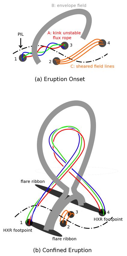
–2–

      Subject headings: Sun: flares — Sun: magnetic topology — Sun: UV radiation
      — Sun: X-rays, gamma rays

                                      1.   Introduction

     The process of a two ribbon flare is usually described by the CSHKP or the standard
flare model (Carmichael 1964; Sturrock 1966; Hirayama 1974; Kopp & Pneuman 1976),
which has been extended in various ways by many authors. The generally accepted view is
summarized below. Before the occurrence of a flare, a core field with highly sheared field
lines or a magnetic flux rope lies below the overlying arched envelope field. Due to the
onset of a magnetic instability, the core field starts to rise and stretches the envelope field to
form a current sheet below it. The magnetic reconnection in the current sheet converts the
magnetic energy into kinetic and thermal energies of plasma and particles, which propagate
along the reconnected field lines below the reconnection site and generate soft X-ray loops
along the magnetic arcades and hard X-ray (HXR) sources at the footpoints of the loops.
The magnetic reconnection site moves upward as the reconnection proceeds, which generates
new soft X-ray loop shells above the older ones that have cooled down to extreme ultraviolet
(EUV) and Hα loops. The intersection of the loop system with the chromosphere and
transition region displays the pattern of flare ribbons. The eruption of the magnetic flux
rope above the reconnection site may propel plasma into the interplanetary space and form
a coronal mass ejection (CME) if the eruption is not confined to the low corona (because of
a too strong overlying magnetic arcade).
     However, there is one puzzling problem in the observations of flare ribbons and HXR
sources at the loop footpoints. While flare ribbons observed in ultraviolet (UV) and Hα
bands appear as elongated brightening structures on both sides of a polarity inversion line of
the associated line-of-sight magnetic field, ribbon-like HXR sources have only been reported
in very rare cases (Masuda et al. 2001; Liu et al. 2007a; Jing et al. 2007). Most HXR sources
appear as compact point-like sources. The problem of lacking ribbon-like HXR sources is
explained by the fact that electrons are most efficiently accelerated in particular loops due to
fast reconnection rate; therefore, weak HXR emissions cannot be recorded by present HXR
instruments with limited dynamic ranges (Asai et al. 2002; Temmer et al. 2007; Miklenic
et al. 2007). But the reason is still not clear why the reconnection rate is faster in that
particular site.
    Magnetic flux ropes serve as a promising candidate to produce HXR sources, since
they play an important role in models of solar active phenomena including flares, fila-
ments/prominences, and CMEs. There is more and more evidence showing that magnetic
–3–
reconnection could also occur in the leading edge of an erupting flux rope, in addition to
the classical current sheet tracing behind and stretched by it, both from observations (Ji
et al. 2003; Wang et al. 2009; Huang et al. 2011) and from numerical simulations (Amari
et al. 2003; Roussev et al. 2003; Török & Kliem 2005). Especially, Wang et al. (2009) found
that EUV brightenings always appear at the two far footpoints of erupting filaments with
the Extreme-ultraviolet Imaging Telescope (EIT; Delaboudinière et al. 1995) on board the
Solar and Heliospheric Observatory (SOHO) in regions of the quiescent Sun. This finding
motivates us to study erupting flux ropes in active regions and to check if any brighten-
ings appear at their footpoints. Moreover, we need to study the relationship between HXR
sources and the flare ribbons.
The HXR and UV emissions in a flare are generated by energetic particles via different
radiation mechanisms. The high energy particles are accelerated in a suitable environment
produced by magnetic reconnection, which occurs preferably at magnetic null points, sepa-
ratrices, or at least Quasi-Separatrix Layers (QSLs). QSLs refer to thin irregular volumes
where the mapping of field lines, e.g. to the photosphere, has a drastic change for a given
three dimensional magnetic field. QSLs divide the magnetic field into different domains.
These domains, however, may be continuously connected at some locations. This is different
from separatrices associated to magnetic null points, where different domains are totally
topologically distinct.
Démoulin et al. (1996) proposed a method to compute the locations of QSLs. Given a
three dimensional magnetic field in a volume, one integrates a field line from P (x, y, z) to
both directions with a distance s on each side. Taking two points (x′ , y ′ , z ′ ) and (x′′ , y ′′, z ′′ )
on both ends of the field line, a vector can be defined as D(x, y, z) = {X1 , X2 , X3 } =
{x′′ − x′ , y ′′ − y ′ , z ′′ − z ′ }. The vector D(x, y, z) changes drastically in QSLs given a small
displacement of point P (x, y, z). Thus, if the norm N is defined as
v "
u 2 2 2 #
uX ∂X i ∂X i ∂X i
N(x, y, z, s) = t + + , (1)
i=1,3
∂x ∂y ∂z
QSLs are field lines with N ≫ 1. In a practical numerical computation, we need to compute
N at each point in a volume, which is very time consuming. Therefore, Démoulin et al.
(1996) suggested to compute a fixed number of points from a coarse grid to finer and finer
grids.
Equation (1) can be further simplified if one limits the positions of the two ends with
more restrictions. For instance, if they are line-tied on the photosphere where z ′ = z ′′ = 0,
the partial derivatives of X3 to any coordinate equal zero, and the footpoints of a field line
only depend on x and y (but not z). Then, the partial derivatives of Xi (i = 1, 2, 3) to z are–4–
zero and Equation (1) is reduced to
s 2 2 2 2
∂X∓ ∂X∓ ∂Y∓ ∂Y∓
N± ≡ N(x± , y± ) = + + + , (2)
∂x± ∂y± ∂x± ∂y±
where {X∓ , Y∓ } = {x∓ − x± , y∓ − y± } (Priest & Démoulin 1995). Titov et al. (2002) pointed
out that N+ does not always equal to N− for the same field line, which are computed at
the footpoints of the same field line, (x+ , y+ ) and (x− , y− ), respectively. They proposed the
squashing degree Q as the measure of field line mapping, and
N+2 N−2
Q= = , (3)
|Bn+ /Bn− | |Bn− /Bn+ |
where Bn+ and Bn− are the normal components of the magnetic field at the two ends of a
field line. The advantage to define the squashing degree Q instead of the norm N is that it
is symmetric in computations at both footpoints of a field line. QSLs are then defined as
those field lines with Q ≫ 2.
The M1.1 flare in active region NOAA 10767 on 2005 May 27 is a good sample for us to
study the relationship between HXR sources and UV ribbons. Guo et al. (2010b) has found
a magnetic flux rope and dipped magnetic arcades coexisting along the Hα filament in the
active region with the nonlinear force-free field model. The chirality of the filament barb
is left bearing in the magnetic arcade section with negative magnetic helicity, which would
induce a filament barb with right bearing in the flux rope section with the same magnetic
helicity. Guo et al. (2010a) found that the eruption of the flux rope was confined in the
corona. With a detailed analysis on the twist number and decay index of the background
magnetic field, Guo et al. (2010a) concluded that the eruption was triggered and initially
driven by the kink instability, but the background magnetic field did not decrease fast enough
with height, thus prevented the occurrence of an ejective eruption with an CME.
In this paper, we study the HXR and UV emissions of the M1.1 flare on 2005 May
27. Particularly, we try to find their temporal and spatial relationships and to link these
emissions with the three dimensional magnetic field structure, i.e. the computed flux rope
and QSLs. Observations and data analysis are described in Section 2. Results are presented
in Section 3. We discuss our findings in Section 4 and draw our conclusions in Section 5.
2. Observations and Data Analysis
The M1.1 flare that occurred in active region NOAA 10767 on 2005 May 27 was observed
uninterruptedly by the Transition Region and Coronal Explorer (TRACE ; Handy et al. 1999)–5–
in the 1600 Å band with a cadence of ∼30 s during the whole flare time. We calibrate the
observed data by subtraction of the detector dark current and normalization with the flat
field and the exposure time. The final derived data are in units of DN s−1 pixel−1 . The X-ray
observations of the M1.1 flare were obtained by the Ramaty High Energy Solar Spectroscopic
Imager (RHESSI ; Lin et al. 2002), which is a space-borne instrument that provides imaging
spectroscopy observations both in X-rays and gamma rays from 3 keV to 17 MeV. Nine
rotating collimators with two grids at both ends of each collimator convert the spatial image
of the Sun into the temporal modulation of the photon counts, which are recorded by nine
germanium detectors respectively with high energy resolution (.1 keV at 3 keV to ∼5 keV
at 5 MeV). The detailed analysis of X-ray data is described in the following section.
2.1. RHESSI Imaging and Imaging Spectroscopy
Figure 1a displays the soft X-ray flux obtained by Geostationary Orbiting Environmental
Satellites (GOES ) 12, showing that the M1.1 flare peaked at ∼12:30 UT on 2005 May 27.
The HXR count rates measured by RHESSI at higher energy bands (i.e., 25.0–50.0 keV)
reached their peaks at ∼12:28 UT as shown in Figure 1b, about 2 minutes earlier than the
peaks at the soft X-ray (SXR) bands. Such a time evolution behavior is due to the Neupert
effect, i.e., the integral of the non-thermal fluxes coincides with the thermal fluxes. We have
checked the time derivative of the GOES flux at 1.0–8.0 Å and the RHESSI flux curve at
25.0–50.0 keV. Their peaks coincide with each other very well, which justifies the Neupert
effect. We fit the spectra with thermal and non-thermal components in fifteen 20-second
accumulation intervals from 12:25:20–12:30:20 UT. It is found that the spectral indices in
the non-thermal component display a typical soft-hard-soft evolution.
We plot the X-ray images reconstructed from RHESSI observations with the clean
method in three energy bands (6.0–12.0, 12.0–25.0, and 25.0–50.0 keV) and three time in-
tervals around the peak of the M1.1 flare in Figure 2. The figure shows that both footpoints
appeared at the middle time. Only the eastern footpoint was present at all the three en-
ergy bands one minute before and after the middle time except the energy band of 6.0–12.0
keV at 12:28:20–12:28:40 U. In each of the three energy bands, the eastern and the western
footpoints display different evolution behaviors in flux. The flux of the eastern footpoint
increases monotonically in all the three energy bands with time, while the flux of the west-
ern footpoint increases monotonically only in the energy band of 6.0–12.0 keV (Figure 2).
Indeed, the flux of the western footpoint first increases and then decreases in the other two
energy bands. Finally, in the time interval of of 12:27:20–12:27:40 UT and in the lower en-
ergy band (6.0–12.0 keV), the flux at the eastern footpoint is larger than that at the western–6–
one, while the situation is reversed in the higher energy band (25.0-50.0 keV, see the central
row in Figure 2).
To give a quantitative measurement of the non-thermal spectra at each footpoint, the
photon fluxes are integrated for sub-regions enclosed by the boxes as shown in the middle
row of Figure 2 for different time intervals and energy bands. We use 20-second accumulation
intervals and 11 energy bands between 10 and 120 keV. We find that the flux versus energy
relationship can be well fitted by a power law for fifteen time intervals within 12:25:20–
12:30:20 UT at the eastern footpoint; but at the western footpoint, it can only be fitted for
six time intervals within 12:26:40–12:28:40 UT. Figure 3 shows the observed X-ray spectra
and their fittings as an example. The non-thermal spectra for both the eastern and the
western footpoints exhibit a soft-hard-soft evolution around the peak of the flare. If we
assume that the photon flux has a power law form, F (E) ∼ E −δ , the power law index δ
reaches the smallest value of 3.9 in the time interval of 12:26:40–12:27:00 UT for the eastern
footpoint, and of 3.6 in the time interval of 12:27:20–12:27:40 UT for the western footpoint.
Therefore, the HXR spectra become the hardest at different times for different footpoints.
2.2. Magnetic Field Extrapolations
In order to compute QSLs, we construct a three dimensional magnetic field as shown
in Figure 4 with the potential field model using the line-of-sight magnetic field observed by
the Michelson Doppler Imager (MDI; Scherrer et al. 1995) on board SOHO. The northern
active region NOAA 10766 and the southern one NOAA 10767 were observed at 11:11 UT
on 2005 May 27. Guo et al. (2010b) have analyzed active region NOAA 10767 by the non-
linear force-free field model. The bottom boundary is the vector magnetic field obtained by
the Télescope Héliographique pour l’Etude du Magnétisme et des Instabilités Solaires/Multi-
Raies (THEMIS /MTR; Bommier et al. 2007). The field lines of the flux rope obtained by
the nonlinear force-free field model are overlaid with the potential field to show both the
large and small scales of the magnetic field structure. Yet, we have not tried to construct a
combined model incorporating both the nonlinear force-free field and the potential field here.
Only selected field lines from both models are overlaid on the same figure for illustration.
As shown in Figure 5, the M1.1 flare occurred in the southern active region, which is
connected to the northern one by the trans-equatorial field lines (Figure 4a). In a thin layer
at the border of this region with trans-equatorial connections, field lines have a drastic change
of their linkages. We show in Figure 6 that this thin layer is a QSL. Finally, from Figure 4b
and 4c, we find that the region with highly twisted field lines is relatively small compared
to the region covered with the surrounding arcade which extends up to the previous QSL.–7–
2.3. Coalignment of the Data
We compare the RHESSI observation with the TRACE 1600 Å image at the peak time
of the M1.1 flare to check if the two HXR sources are conjugate footpoints of a flare. The
two images have to be aligned with each other to compare their features. Because RHESSI
observes the full disk, the coordinates of the observed targets can be computed via the
comparison of the positions of the solar limbs. The accuracy is within the spatial resolution
of RHESSI observations, which is 7′′ for images reconstructed from the six detectors 3F–8F.
MDI also observes the full disk so that the coordinates of MDI observations can be precisely
determined (with an error around its spatial resolution of 2′′ ).
The TRACE image can be aligned with the magnetic field observed by THEMIS by
comparing the positions of the erupting feature in the 1600 Å band before the flare peak with
the pre-eruptive flux rope found by the extrapolation (as shown in Figure 5a). Magnetic
fields observed by THEMIS and MDI are aligned by comparing their common features of
the line-of-sight magnetic field. Thus, the TRACE 1600 Å image is aligned with the MDI
observation. The alignment accuracy is estimated to be about 2′′ , which is roughly the
spatial resolution of MDI; by comparison, TRACE and THEMIS have much higher spatial
resolutions of 0.5′′ and 0.8′′ , respectively. The pointing offset of the TRACE 1600 Å image
can be used through the whole flare process after considering the solar rotation, since the
pointing error was small during such a relatively short time range. Finally, the RHESSI
HXR image is aligned with the TRACE 1600 Å image as shown in Figure 5c. Contours of
the line-of-sight magnetic field, which were observed by THEMIS /MTR at 10:17 UT on 2005
May 27 and differentially rotated to 12:27 UT, are overlaid on both RHESSI and TRACE
images.
3. Results
3.1. Initial Presence and Development of a Flux Rope
Guo et al. (2010b) found a small flux rope in this active region about 2 hours before the
peak of the flare by the nonlinear force-free field extrapolation method (Wheatland et al.
2000; Wiegelmann 2004). The magnetic flux rope corresponded to the eastern part of an
Hα filament, whose western part was found by the magnetic extrapolation to be supported
by sheared magnetic arcades. From the beginning of the flare, a first type of reconnection
(called R1 hereafter) occurred nearby the flux rope. The consequence of such reconnection
is the development of a bright feature along the polarity inversion line (see Figure 5a and
the attached movie). As shown in Figure 5a, we find that the UV brightening generated by–8–
magnetic reconnection appeared nearby the pre-eruptive flux rope.
During the peak time of the confined eruption, the erupting magnetic flux rope, as
suggested by the TRACE 1600 Å observation, was much longer than that at the eruption
onset, as found by the nonlinear force-free field extrapolation. Magnetic reconnection (called
R2 hereafter) might occur between the magnetic flux rope and the sheared arcades to form
a longer flux rope, which facilitated the further eruption and the reconnection in the main
phase. However, the above scenario should be taken with caution, since different nonlinear
force-free field algorithms could not obtain a unique solution with observational data as the
bottom boundary (e.g., DeRosa et al. 2009). Thus, we need to compare an extrapolated
magnetic field with more observations, such as Hα filaments and/or TRACE 171 Å loops.
Guo et al. (2010b) showed that the magnetic dips in the nonlinear force-free field model
coincided with the locations of the associated Hα filament, which is a test of the extrapolation
result.
In order to find the evidence of the reconnection R2, it is better to check the HXR image
evolution. Unfortunately, there were no RHESSI data during 11:54–12:25 UT and there was
no clear evidence showing the onset reconnection at the center of the region in other time
intervals. A bump on the GOES flux curve at 12:15 UT (Figure 1a) shows an indirect
evidence of energy release; however, we do not know where it comes from. Only the TRACE
1600 Å observation covered this active region during the flare. From these observations we
find that there was no brightening at the location where the flux rope contacted with the
sheared arcades before 12:00 UT. Next, we integrate the TRACE 1600 Å flux in the region
surrounded by a box as plotted in Figure 5a. The selected box tracks the region where the
magnetic flux rope and the sheared arcades contacted with each other and follows the solar
rotation. The integrated flux curve is in the time range of 12:00–13:00 UT. As shown in
Figure 5d, a small peak appeared at 12:14 UT before the main peak of the integrated flux.
Recall that at almost the same time, GOES recorded a small bump in the SXR flux. The
coincidence of the peak time suggests that the SXR emission was generated in the same
region as that of the 1600 Å band, implying further that magnetic reconnection R2 possibly
occurred at the center of the region at ∼12:14 UT (refer to Figure 5b) to form the finally
erupted longer flux rope. The magnetic reconnection between the western magnetic arcades
(tether cutting reconnection to build a larger flux rope, called R3 hereafter) may be initiated
immediately after reconnection R2. There is a possible time overlap when both R2 and R3
were in progress.
We have presented a series of figures and a movie of the TRACE 1600 Å observation in
Guo et al. (2010a) to show the evolution of the helical rope-like structure. A movie showing
the evolutions of TRACE 1600 Å images and RHESSI X-ray sources is included in the–9–
electronic edition of the journal (the flux rope in Figure 5a, the arrows with labels in Figures
5a, 5b, and 5c, and Figure 5e are not shown in the movie). Three snapshots are displayed
in Figures 5a, 5b, and 5c, respectively. It is found that the flare initiated at the location
of pre-eruptive magnetic flux rope (Figure 5a). The small pre-eruptive flux rope grew into
a larger one after the reconnection R2 (Figure 5b). Then, the erupting rope-like structure
displayed an ascending and helically deforming evolution, which is a characteristic of the
kink instability (Figure 5c), thus indicating the existence of a magnetic flux rope throughout
the process of the flare. The rope-like structure stopped to ascend at a certain height and
seemed not to evolve to any CME, suggesting that the eruption was confined in the corona.
3.2. HXR Sources and the Magnetic Flux Rope
Figure 5c shows that the two RHESSI HXR footpoints at 25.0–50.0 keV are located
at the two ends of a helical rope-like structure connecting them. We have concluded that
the helical structure is an erupting flux rope that was formed by magnetic reconnection R2.
Therefore, the HXR sources appeared at the footpoints of the erupting magnetic flux rope.
Figure 5e shows the HXR sources overlaid on an Hα image that was observed about two hours
before the flare, which indicates that the western footpoint of the erupted flux rope is more
extended to the west than the western footpoint of the Hα filament. This shift is coherent
with the western extension of the flux rope during the flare. Both reconnections R2 and
R3 contributed to extend the flux rope to locations where no magnetic dips, so no filament,
were present before the flare. Two types of magnetic reconnection could be responsible for
the generation of these HXR sources: reconnection R3 behind or reconnection (called R4
hereafter) within the erupting flux rope (Figure 5c).
HXR sources at 25.0–50.0 keV first appeared at the eastern footpoint, and the energy
spectra at the two footpoints are different from each other (Section 2.1). The time when the
two HXR sources became the hardest (at ∼12:27 UT) was earlier than the HXR flux peak
time (at ∼12:28 UT), the integrated UV flux peak time (at ∼12:28 UT), and the SXR flux
peak time (at ∼12:30 UT). Different HXR fluxes and spectral indices in the conjugate foot-
points, which is usually termed as asymmetric footpoints, arise from the different properties
in the process of particle acceleration and particle transport (e.g., Liu et al. 2009). Inter-
pretations of conjugate HXR footpoints require a detailed study of the particle acceleration
mechanism, magnetic mirroring effect, column density of the flare loops and other effects,
which is out of the scope of this paper.– 10 –
3.3. Flare Ribbons and Quasi-Separatrix Layers
A TRACE 1600 Å image at 12:14 UT, when the flare ribbons clearly appeared, is
overlaid with the potential field lines that are rotated to the TRACE observation time as
shown in Figure 6a. The intersection of computed QSLs and the photosphere is overlaid
on the TRACE 1600 Å image in Figure 6b. The selected TRACE observation time is close
to the first peak of the UV flux (Figure 5d) in the central area, so it was taken when
reconnection R2 was occurring. The northwestern ribbon has a distance of more than 5′′ to
the location of the QSL intersection on the photosphere, which indicates that no field lines
in the QSL computed with the potential field extrapolation were involved in the magnetic
reconnection to produce the flare ribbons, in contrast with many previous studies which
related flare ribbons to QSLs (see, e.g., Démoulin 2007, and references therein). In fact,
the QSLs involved in R1 (and later in R2 and R3) are associated to the presence of the
erupting flux rope, which are not present in the potential field extrapolation of Figure 6.
The potential-field QSLs are privilege locations of the concentrated current layers if there
is enough magnetic field evolution in these regions (Aulanier et al. 2005). The absence of
significant brightenings at the potential-field QSLs implies that the driving force by the
distant erupting flux rope was not enough to build thin enough current layers (to be able to
provide significant reconnection, so significant energy release).
As the flare proceeded, the flare ribbons separated apart. We overlay the potential field
lines and the intersection of the potential-field QSLs on the TRACE 1600 Å image at 12:47
UT, the late phase of the flare (Figures 6c and 6d). The right part of the northwestern ribbon
stopped at the border of the QSL, while the left stopped before reaching it. We interpret
this result as follows. If a magnetic flux rope is ejected into the interplanetary space, the
overlying arcade is fully stretched. Then, this arcade is expected to be fully reconnected and
further build-up the ejected flux rope. In such a case, reconnection is expected to transform
all the arcade magnetic flux to the flux rope, then the flare ribbons separate up to the arcade
extension. However, if the event is confined, it is expected that a part of the overlying arcade
stays (its downward magnetic tension confines the flux rope). Then, in this latter case, the
flare ribbons are expected to stop their progression before reaching the border of the arcade,
so the associated QSL.
3.4. Summary of the Reconnection Steps
We identify four steps of magnetic reconnection in the process of the flux rope erup-
tion. The first reconnection, R1, occurred nearby the pre-eruptive magnetic flux rope. Since
the flare was observed from above and no height information can be obtained, we cannot– 11 –
determine whether R1 occurred below, within, or above the flux rope from the present ob-
servation. There are some possible reconnection mechanisms for R1. First, It fits the general
picture of the tether-cutting model with the progressive transformation of sheared arcades to
a flux rope. This process is related to the work of Green et al. (2011), where they presented a
detailed study on the flux rope formation and eruption through flux cancellation in another
active region. They showed that a flux rope can be formed by magnetic reconnection before
its eruption. Secondly, magnetic reconnection R1 may occur within the erupting flux rope.
Or finally, the real case can also be the combination of the above two possibilities.
The second reconnection, R2, happened between the small flux rope in the eastern part
of the active region and the sheared magnetic arcades in the western part (Figure 7a). This
step started more than 10 minutes before the main UV and X-ray peaks of the flare. It built
up a longer flux rope and probably stimulated the reconnection within the western sheared
arcades (R3). It implied a western propagation of the flare brightenings along the polarity
inversion line. Such propagation was previously reported in another event (Goff et al. 2007),
and their conclusion (e.g., their Figure 9) is similar to the one presented above.
The fourth step reconnection, R4, is pointed out by the presence of the HXR emission
only at the footpoints of the erupting flux rope. While the spatial resolution and the intensity
saturation of the observations do not permit to exclude that these HXR sources can be formed
by reconnection at the periphery of the growing flux rope (so by reconnection R3), the UV
observations point to a strong energy release within the erupting flux rope.
Finally, the confined eruption of the flux rope did not have a large enough effect on the
large-scale QSLs (computed with a potential field) to build thin enough current layers, so
to induce significant reconnection in the potential-field QSLs (called R5 hereafter), as there
was no significant brightenings associated to these QSLs.
4. Discussion
We summarize the full scenario with a schematic picture in Figure 7, where both the
onset eruption and the final confined eruption are depicted. At the onset of the eruption
as shown in Figure 7a, the magnetic flux rope found by the nonlinear force-free field model
built a highly non-potential state with a twist number exceeding the one suitable for the
helical kink instability, which has been quantitatively analyzed in Guo et al. (2010a). The
helical kink instability is suggested to trigger and drive the eruption. In Guo et al. (2010a),
the authors also found that the final eruption was a confined one, i.e., the eruption of the
magnetic flux rope was constrained within the corona due to the large restoring force of the– 12 –
overlying magnetic field as shown in Figure 7b. In this paper, we have mainly three findings.
First, the HXR sources appeared at the footpoints of a flux rope (as in the events studied
by Liu & Alexander (2009) and Xu et al. (2010)). Secondly, the magnetic reconnection R2
occurred more than 10 minutes before the main peak of the flare. And thirdly, the UV
flare ribbons stopped at the border of the potential-field QSLs. These findings have great
implications on the mechanism and process of the M1.1 flare on 2005 May 27, as discussed
below.
First, we find that the conjugate HXR footpoints at the peak time of the flare were
located at the two footpoints of a magnetic flux rope. This finding is different from the usual
viewpoint, in particular what is based on the two dimensional flare models, where HXR
footpoints are always located at the footpoints of magnetic arcades below the reconnection
site. These arcades are formed by magnetic reconnection of the envelope field, which is
stretched by the erupting flux rope. Such post flare magnetic arcades are mostly potential
and perpendicular to the polarity inversion line, and so cannot provide a magnetic connection
between the two HXR footpoints (Figure 5c and 7b). Such connection can only be provided
by the flux rope connectivity (as deduced from TRACE observations). It implies that high
energy particles are preferably accelerated along the magnetic flux rope. The above results
are related to the results of Cheng et al. (2011). They found in another flare a very hot (∼11
MK) ejected flux rope, which also suggests that a fast and effective heating mechanism is
working.
Does magnetic reconnection only occur at the border of the flux rope or could it occur in
the flux rope body? For the border reconnection case, tether cutting magnetic reconnection
progressively transforms the surrounding arcade field lines to flux rope ones (e.g., Török et al.
2004). So high energy particles and heating are input on all these newly formed field lines.
If the initial flux rope has a small extension compare to the one built up during the eruption,
then most of the erupting flux rope would be filled with hot plasma and high energy particles.
In this process, most energy is provided only at the periphery of the flux rope at a given
time (some energy will be further provided by the latter relaxation of the magnetic field).
Alternately, reconnection within the flux rope could happen with an internal kink instability
Galsgaard & Nordlund (1997); Haynes & Arber (2007). It requires that the twist is large
enough within the flux rope so that the core becomes kink unstable. So far, this internal
kink instability has been proposed only for the heating of coronal loops since the instability
does not affect much the external field (see above references). In the eruption of the flare
on 2005 May 27, an external kink instability is plausibly the cause of the flux rope writhing
as observed by TRACE (Guo et al. 2010a). We further propose here that an internal kink
instability could drive internal reconnection which accelerate high energy particles. In this
case, the HXR sources could be present within the flux rope footpoints, while in the case of– 13 –
tether cutting reconnection they should appear at the border of the footpoints. Due to the
limitation of the spatial resolution of both UV and HXR observations in this study, these
two cases cannot be discriminated.
Next, it is worthwhile to compare our findings with other studies on HXR sources and
UV ribbons in flares. Liu & Alexander (2009) studied the HXR emissions in kinking filaments
for three cases on 2002 May 27, 2003 June 12, and 2004 November 10, respectively. They
found that there are two phases of eruptions, where compact HXR sources appear. In the
first phase the sources appear at the endpoints of the associated filament, and in the second
phase elongated ribbons appear at the footpoints of the magnetic arcades. The authors
proposed that magnetic reconnection occurs between the two writhing filament legs, and
later between the two envelope field legs (in the vertical current sheet) in the two phases,
respectively. Our results are different from Liu & Alexander (2009) in two points. First,
reconnection R1, R2, and R3 lead to the formation of a larger flux rope that caused a confined
eruption later; while in the events of Liu & Alexander (2009), both phases of reconnection
occurred at the time when the flux ropes have fully developed and writhed. Secondly, we
find that the HXR sources coincided with the footpoints of the flux rope at the HXR peak
time. These sources did not move to the footpoints of magnetic arcades formed by magnetic
reconnection in the vertical current sheet as they were observed in the events on 2002 May
27 and 2004 November 10 as shown in Liu & Alexander (2009).
Recently, Xu et al. (2010) found four HXR sources with RHESSI at the onset stage of
an X10 flare on 2003 October 29. The four sources are two conjugate pairs similar to the
ones shown in Figure 7a. This study provides additional evidence for the onset stage with
two steps of magnetic reconnection. However, in our case, there was no observation with
RHESSI at the onset time of the M1.1 flare. The difference between the two studies lies
mainly in the behavior of the HXR sources. In the events of Xu et al. (2010), the two outer
sources (Sources 1 and 4 in Figure 7a) disappeared at the peak time; while in our event, the
two outer sources are the strongest and the two inner sources (Sources 2 and 3) were absent
at the peak time. This difference implies that HXR sources could be formed both at the
footpoints of the flare loops and/or of the erupted flux rope in different environments.
Finally, the northwestern ribbon in the UV 1600 Å band appeared at a location with
a detectable distance to the location of the intersection of the potential-field QSL, and it
stopped nearby the footpoints of the QSL. The intersection of the potential-field QSL on
the photosphere was relatively stable during the impulsive energy release process, since the
shape of flare ribbons during the flaring time still mimic the shape of the QSL intersection
on the photosphere that was observed about one hour before the flare. This is linked to
the confined nature of this eruption, with a flux rope that did not succeed to overcome the– 14 –
downward magnetic tension of its overlying magnetic arcades.
The UV flare ribbons were produced by magnetic reconnection R1, R2, and R3, which
is expected to occur in newly formed current layers during the eruption of the flux rope
(Figure 7b). As pointed out by Chen et al. (2011), the QSLs associated to the above current
layers are difficult to find with the present magnetic field extrapolation method (because it
represents, at best, only the initial configuration). Finally, the erupting field was pushed
close to the large-scale potential-field QSL as the magnetic reconnection proceeded.
5. Conclusions
We study the magnetic field structures of hard X-ray sources and flare ribbons of the
M1.1 flare in active region NOAA 10767 on 2005 May 27. Guo et al. (2010b) has found a
small pre-eruptive magnetic flux rope coexisting with sheared magnetic arcades in a non-
linear force-free field extrapolation. The observations indicate that this flare involved a
multi-reconnection sites, as follows. First, TRACE 1600 Å and GOES SXR fluxes suggest
that an onset magnetic reconnection occurred nearby the flux rope. This reconnection was
triggered and driven by the activation of the pre-eruptive magnetic flux rope, and it further
facilitated the flux rope eruption. Secondly, later on reconnection occurred between the
pre-eruptive magnetic flux rope and sheared magnetic arcades more than 10 minutes before
the flare peak time. Magnetic reconnection steps R2 and R3 provide a possible explana-
tion for the formation of the larger flux rope observed by TRACE. But we cannot exclude
other possibilities due to the limitation of the data available and the nonlinear force-free
field extrapolation. On one hand, there were no HXR observations at the early phase of the
eruption, neither were there any EUV and SXR observations at this phase. On the other
hand, the magnetic filed configuration obtained from the nonlinear force-free field should be
taken with caution as we have discussed in Section 3.1.
RHESSI and TRACE observations show that HXR sources appeared at the footpoints
of the larger flux rope at the peak of the flare. We could not determine whether these sources
were created by particles accelerated within or nearby the border of the large flux rope. Still,
the spatial coincidence between the HXR sources and the footpoints of the flux rope favors
particle acceleration within the flux rope. A possible mechanism could be the development
of an internal kink instability, since it would induce the formation of a thin current layer,
then of reconnection, within the flux rope.
Finally, a topological analysis of a large solar region including the active regions NOAA
10766 and 10767 shows the existence of large-scale QSLs before the eruption of the flux rope.– 15 –
Such QSLs did not participate in the flare, but the extension of the flare ribbons is found to
be confined inside the closest large-scale QSL computed from a potential field extrapolation.
We conclude that the reconnection, involved in the confined eruption of the flux rope, was not
involving larger scale structures than the arcade overlying the flux rope. The northwestern
ribbon ended along the closest QSL computed with the potential field from a magnetogram
taken before the flare. Such spatial coincidence indicates that the magnetic field should not
deviate much from the potential field in the envelope field far from the core field region.
The nonlinear force-free field model from the optimization method as derived in Guo et al.
(2010b) has a smaller spatial extention than the above potential field extrapolation because
of the limited field of view of the vector magnetogram available. Still, the nonlinear model
indicates that the magnetic field gradually gets closer to the potential field as the distance
from the center of the active region increases. Together with the good correspondence found
previously between the extensions of the computed magnetic dips and the Hα filament, this
is a confirmation that the nonlinear force-free field model provides a reliable approximation
of the coronal field.
The authors thank the referee for helpful comments that improved the clarity of the
paper. Y.G. thanks Pengfei Chen very much for useful discussions. We are grateful to the
GOES, RHESSI, SOHO, THEMIS, and TRACE teams for providing the valuable data. Y.G.
and M.D.D. are supported by NSFC under grants 10828306 and 10933003, and by NKBRSF
under grant 2011CB811402. The research leading to these results has received funding from
the European Commission’s Seventh Framework Programme (FP7/2007-2013) under the
grant agreement No. 218816 (SOTERIA project, www.soteria-space.eu). H.L. is supported
by NSFC under grants 10873038 and 10833007, and by NKBRSF under grant 2011CB811402.
REFERENCES
Amari, T., Luciani, J. F., Aly, J. J., Mikic, Z., & Linker, J. 2003, ApJ, 595, 1231
Asai, A., Masuda, S., Yokoyama, T., Shimojo, M., Isobe, H., Kurokawa, H., & Shibata, K.
2002, ApJ, 578, L91
Aulanier, G., Pariat, E., & Démoulin, P. 2005, A&A, 444, 961
Bommier, V., Landi Degl’Innocenti, E., Landolfi, M., & Molodij, G. 2007, A&A, 464, 323
Carmichael, H. 1964, NASA Special Publication, 50, 451
Chen, P. F., Su, J. T., Guo, Y., & Deng, Y. Y. 2011, ArXiv e-prints– 16 –
Cheng, X., Zhang, J., Liu, Y., & Ding, M. D. 2011, ApJ, 732, L25
Delaboudinière, J. et al. 1995, Sol. Phys., 162, 291
Démoulin, P. 2007, Advances in Space Research, 39, 1367
Démoulin, P., Hénoux, J. C., Priest, E. R., & Mandrini, C. H. 1996, A&A, 308, 643
DeRosa, M. L. et al. 2009, ApJ, 696, 1780
Galsgaard, K. & Nordlund, Å. 1997, J. Geophys. Res., 102, 219
Goff, C. P., van Driel-Gesztelyi, L., Démoulin, P., Culhane, J. L., Matthews, S. A., Harra,
L. K., Mandrini, C. H., Klein, K. L., & Kurokawa, H. 2007, Sol. Phys., 240, 283
Green, L. M., Kliem, B., & Wallace, A. J. 2011, A&A, 526, A2
Guo, Y., Ding, M. D., Schmieder, B., Li, H., Török, T., & Wiegelmann, T. 2010a, ApJ, 725,
L38
Guo, Y., Schmieder, B., Démoulin, P., Wiegelmann, T., Aulanier, G., Török, T., & Bommier,
V. 2010b, ApJ, 714, 343
Handy, B. N. et al. 1999, Sol. Phys., 187, 229
Haynes, M. & Arber, T. D. 2007, A&A, 467, 327
Hirayama, T. 1974, Sol. Phys., 34, 323
Huang, J., Démoulin, P., Pick, M., Auchère, F., Yan, Y. H., & Bouteille, A. 2011, ApJ, 729,
107
Ji, H., Wang, H., Schmahl, E. J., Moon, Y., & Jiang, Y. 2003, ApJ, 595, L135
Jing, J., Lee, J., Liu, C., Gary, D. E., & Wang, H. 2007, ApJ, 664, L127
Kopp, R. A. & Pneuman, G. W. 1976, Sol. Phys., 50, 85
Lin, R. P. et al. 2002, Sol. Phys., 210, 3
Liu, C., Lee, J., Gary, D. E., & Wang, H. 2007a, ApJ, 658, L127
Liu, C., Lee, J., Yurchyshyn, V., Deng, N., Cho, K.-S., Karlický, M., & Wang, H. 2007b,
ApJ, 669, 1372
Liu, R. & Alexander, D. 2009, ApJ, 697, 999– 17 –
Liu, W., Petrosian, V., Dennis, B. R., & Holman, G. D. 2009, ApJ, 693, 847
Masuda, S., Kosugi, T., & Hudson, H. S. 2001, Sol. Phys., 204, 55
Miklenic, C. H., Veronig, A. M., Vršnak, B., & Hanslmeier, A. 2007, A&A, 461, 697
Moore, R. L., Sterling, A. C., Hudson, H. S., & Lemen, J. R. 2001, ApJ, 552, 833
Priest, E. R. & Démoulin, P. 1995, J. Geophys. Res., 100, 23443
Roussev, I. I., Forbes, T. G., Gombosi, T. I., Sokolov, I. V., DeZeeuw, D. L., & Birn, J.
2003, ApJ, 588, L45
Scherrer, P. H. et al. 1995, Sol. Phys., 162, 129
Sturrock, P. A. 1966, Nature, 211, 695
Temmer, M., Veronig, A. M., Vršnak, B., & Miklenic, C. 2007, ApJ, 654, 665
Titov, V. S., Hornig, G., & Démoulin, P. 2002, J. Geophys. Res. (Space Phys.), 107, 1164
Török, T. & Kliem, B. 2005, ApJ, 630, L97
Török, T., Kliem, B., & Titov, V. S. 2004, A&A, 413, L27
Wang, Y., Muglach, K., & Kliem, B. 2009, ApJ, 699, 133
Wheatland, M. S., Sturrock, P. A., & Roumeliotis, G. 2000, ApJ, 540, 1150
Wiegelmann, T. 2004, Sol. Phys., 219, 87
Xu, Y., Jing, J., Cao, W., & Wang, H. 2010, ApJ, 709, L142
This preprint was prepared with the AAS LATEX macros v5.2.– 18 – Fig. 1.— (a) Soft X-ray flux from the GOES 12 satellite of the M1.1 flare on 2005 May 27. Dashed and dash-dotted lines indicate two peaks of the X-ray flux. The two arrows denote the time range of the RHESSI light curve shown below. (b) Corrected X-ray light curve obtained by RHESSI. The peaks at different energy bands started at around 12:35, 12:40, and 12:44 UT are instrumental artifacts caused by removing the thicker attenuator before the detectors.
– 19 –

Fig. 2.— X-ray images reconstructed from RHESSI observations with the clean method in
three energy bands (6.0–12.0, 12.0–25.0, and 25.0–50.0 keV) and three time intervals close to
the peak of the M1.1 flare on 2005 May 27. The color-flux scale is the same in each column,
but different within each row. Six detectors (3F–8F) are selected to reconstruct the images.
The white boxes in the middle row enclose the regions in which the photon flux is integrated
to build the spectra (Figure 3).
– 20 –

Fig. 3.— Observed hard X-ray spectra with vertical and horizontal error bars showing the
errors in the flux and the width of energy bins, respectively. The spectra are constructed in
the regions enclosed by the rectangular boxes as shown in Figure 2. They are fitted by a
power law function (solid line), with the absolute value of the power index δ shown in each
panel. Top and bottom rows show the spectra at two time intervals, i.e., 12:26:40–12:27:00
UT and 12:27:20–12:27:40 UT, respectively. The two vertical dashed lines in each panel
indicate the fitting energy ranges. The normalized residuals are shown at the bottom of each
panel.
– 21 –

Fig. 4.— Potential field extrapolation using MDI line-of-sight magnetogram observed at
11:11 UT on 2005 May 27. The flux rope is extrapolated by the nonlinear force-free field
model with the vector magnetic fields observed by THEMIS /MTR at 10:17 UT on 2005
May 27. The field lines of the flux rope are overlaid with the potential field after rotating
the coordinates to the MDI observation time. Different panels show different fields of views
and viewing angles.
– 22 –

Fig. 5.— (a) TRACE 1600 Å image (the gray scale is reversed) at 12:07 UT overlaid by
the pre-eruptive flux rope and some selected sheared field lines, which have been rotated
to the observation time of the TRACE image. Solid, dashed, and dash-dotted contours
denote respectively the positive, negative polarities, and the polarity inversion line of the
line-of-sight magnetic field observed by THEMIS /MTR at 10:17 UT on 2005 May 27 and
rotated differentially to the observation time of the TRACE image. The arrow points to a
brightening region in the TRACE 1600 Å image. The labels Ri (i = 1–4) are reconnection
steps defined in Section 3.4. (b) TRACE 1600 Å image at 12:14 UT. (c) TRACE 1600 Å
image at the HXR peak time of the M1.1 flare overlaid by the RHESSI X-ray contours. The
integration time interval for the X-ray image is 12:27:20–12:27:40 UT. (d) TRACE 1600 Å
flux integrated in the rectangular box as shown in previous panels. Dashed and dash-dotted
lines indicate the two peaks of the integrated flux. (e) An Hα filament overlaid by the
RHESSI X-ray contours as that in panel (c) and being rotated to the observation time of
the Hα filament. (f) The Hα filament observed by THEMIS /MTR on 2005 May 27.

(An mpeg animation is available in the electronic edition of the journal.)
– 23 –

Fig. 6.— (a) TRACE 1600 Å image at 12:14 UT overlaid with potential field lines at 11:11
UT, which have been rotated to the TRACE observation time. (b) TRACE 1600 Å image
at 12:14 UT overlaid with the intersection of QSLs with the photosphere. The QSLs are
calculated with the potential field extrapolated with the MDI line-of-sight magnetogram at
11:11 UT. Only the QSL intersections with Q ≥ 104 are shown as the hatched area. (c)
TRACE 1600 Å image at 12:47 UT overlaid with potential field lines at 11:11 UT, which
have been rotated to the TRACE observation time. (d) TRACE 1600 Å image at 12:47 UT
overlaid with the intersection of QSLs with the photosphere. The QSLs are the same to that
in panel (b).
– 24 –

Fig. 7.— Schematic picture of the onset and final stage of the confined eruption. The idea
is based on the tether-cutting model of Moore et al. (2001). This picture can be compared
with the one for the ejective eruption in Liu et al. (2007b).
You can also read