Understanding performance and obtaining hardware information - December 11, 2018 Robert Sinkovits - San Diego ...
←
→
Page content transcription
If your browser does not render page correctly, please read the page content below

Understanding performance and obtaining
         hardware information
                       December 11, 2018
                        Robert Sinkovits

     SAN DIEGO SUPERCOMPUTER CENTER

                                      at the UNIVERSITY OF CALIFORNIA; SAN DIEGO
Code of Conduct

XSEDE has an external code of conduct for XSEDE sponsored events
which represents XSEDE's commitment to providing an inclusive and
harassment-free environment in all interactions regardless of gender,
sexual orientation, disability, physical appearance, race, or religion. The
code of conduct extends to all XSEDE-sponsored events, services, and
interactions.

Code of Conduct: https://www.xsede.org/codeofconduct

Contact:
• Event organizer: Robert Sinkovits (sinkovit@sdsc.edu)
• XSEDE ombudspersons:
    • Linda Akli, Southeastern Universities Research Association,
       (akli@sura.org)
    • Lizanne Destefano, Georgia Tech
       (lizanne.destefano@ceismc.gatech.edu)
    • Ken Hackworth, Pittsburgh Supercomputing Center,
       (hackworth@psc.edu)

        SAN DIEGO SUPERCOMPUTER CENTER
                                                                                        2
                                           at the UNIVERSITY OF CALIFORNIA; SAN DIEGO
Background and clarifications

The material for this webinar was adapted from presentations at the 2018
SDSC Summer Institute. Total presentation time was about five hours and
this webinar distills some of the key points into a 75 minute time slot. For
the full presentations, please see

https://github.com/sdsc/sdsc-summer-institute-2018

https://github.com/sdsc/sdsc-summer-institute-
2018/tree/master/6_software_performance

https://github.com/sdsc/sdsc-summer-institute-
2018/tree/master/hpc1_performance_optimization

         SAN DIEGO SUPERCOMPUTER CENTER
                                                                                       3
                                          at the UNIVERSITY OF CALIFORNIA; SAN DIEGO
Background and clarifications (part 2)

And I realized belatedly that there is some discrepancy between the title,
abstract and what I intended to cover in this webinar. Today, we’ll focus
more on obtaining hardware information (per the title) and touch lightly on
optimization

• Why would I want to obtain hardware and system information?
• How do I get info such as CPU specs, memory quantity, cache
  configuration, file systems, OS version, GPU properties, etc?
• Two simple tools for profiling codes and monitoring system usage
• The memory hierarchy
• An example of optimizing for cache

         SAN DIEGO SUPERCOMPUTER CENTER
                                                                                       4
                                          at the UNIVERSITY OF CALIFORNIA; SAN DIEGO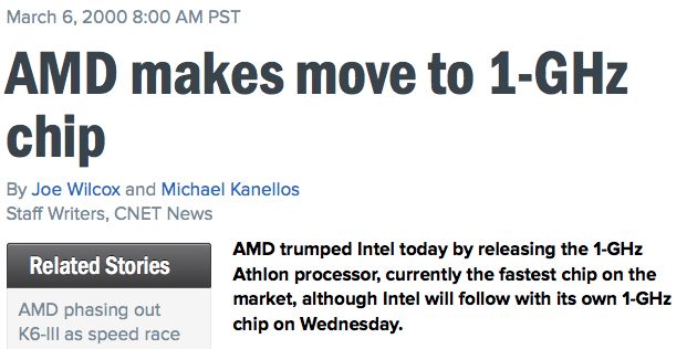
Introduction

• Most of you are here because you are computational scientists and
  users of HPC systems (i.e. software rather than hardware people)
• But it’s still worth an hour of your time to learn something about
  hardware since it will help you become a more effective computational
  scientist
• As a bonus, just about everything that we cover today will be widely
  applicable, from most XSEDE resources to your local Linux cluster

        SAN DIEGO SUPERCOMPUTER CENTER
                                                                                      5
                                         at the UNIVERSITY OF CALIFORNIA; SAN DIEGO
Getting hardware info – why should I care?
•   You may be asked to report the details of your hardware in a manuscript,
    presentation, proposal or request for computer time. This is especially important
    if you’re discussing application performance

•   You’ll know exactly what you’re running on. Can answer questions like “Is the
    login node the same as the compute nodes?” or “How does my local cluster
    compare to the nodes on the supercomputers”

•   It will give you a way of estimating performance, or at least bounds on
    performance, on another system. All else being equal, jobs will run at least as
    fast on hardware that has
       • Faster CPU clock speeds
       • Larger caches
       • Faster local drives

•   You’ll sound smart when you talk to other technical people ;)

           SAN DIEGO SUPERCOMPUTER CENTER
                                                                                            6
                                               at the UNIVERSITY OF CALIFORNIA; SAN DIEGO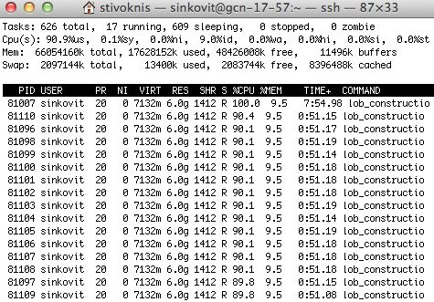
Getting processor information (/proc/cpuinfo)
On Linux machines, the /proc/cpuinfo pseudo-file lists key processor information.
Mostly cryptic hardware details, but also some very helpful data
processor        :   0 (processor number, actually refers to core)
vendor_id        :   GenuineIntel
cpu family       :   6
model            :   63
model name       :   Intel(R) Xeon(R) CPU E5-2680 v3 @ 2.50GHz (processor type)
stepping         :   2
Microcode        :   50
cpu MHz          :   2501.000 (nominal clock speed)
cache size       :   30720KB
physical id      :   0
siblings         :   12
core id          :   0
cpu cores        :   12 (number of cores in processor)
apicid           :   0
initial apicid   :   0
fpu              :   yes
fpu_exception    :   yes
cpuid level      :   15
wp               :   yes
flags            :   fpu vme de … avx … avx2 (AVX/AVX2 capable processor)

          SAN DIEGO SUPERCOMPUTER CENTER
                                                                                             7
                                                at the UNIVERSITY OF CALIFORNIA; SAN DIEGO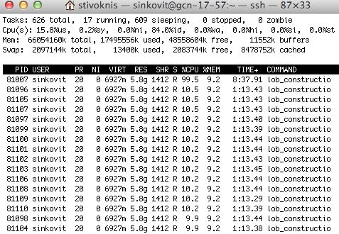
Getting processor information (/proc/cpuinfo)
If you want to find out how many processors or cores you have on the compute
node, grep for ‘processor’ or ‘physical id’
  $ grep processor /proc/cpuinfo              $ grep 'physical id' /proc/cpuinfo
  processor : 0                               physical id : 0
  processor : 1                               physical id : 0
  processor : 2                               physical id : 0
  processor : 3                               physical id : 0
  processor : 4                               physical id : 0
  processor : 5                               physical id : 0
  processor : 6                               physical id : 0
  processor : 7                               physical id : 0
  processor : 8                               physical id : 0
  processor : 9                               physical id : 0
  processor : 10                              physical id : 0     cores 0-11 are on
  processor : 11                              physical id : 0     socket 0 and 12-23
  processor : 12                              physical id : 1     are on socket 1
  processor : 13                              physical id : 1
  processor : 14                              physical id : 1
  processor : 15                              physical id : 1
  processor : 16                              physical id : 1
  processor : 17                              physical id : 1
  processor : 18                              physical id : 1
  processor : 19                              physical id : 1
  processor : 20                              physical id : 1
  processor : 21                              physical id : 1
  processor : 22                              physical id : 1
  processor : 23                              physical id : 1

                                   Results shown are for Comet standard compute node

           SAN DIEGO SUPERCOMPUTER CENTER
                                                                                              8
                                                 at the UNIVERSITY OF CALIFORNIA; SAN DIEGO
Getting processor information (/proc/cpuinfo)
If you want to find out how many processors or cores you have on the compute
node, grep for ‘processor’ or ‘physical id’
$ grep processor /proc/cpuinfo $ grep 'physical id' /proc/cpuinfo
processor : 0 physical id : 0
processor : 1 physical id : 1
processor : 2 physical id : 0
processor : 3 physical id : 1
processor : 4 physical id : 0
processor : 5 physical id : 1
processor : 6 physical id : 0
processor : 7 physical id : 1
processor : 8 physical id : 0
processor : 9 physical id : 1
processor : 10 physical id : 0
cores are assigned
processor : 11 physical id : 1 round-robin to
processor : 12 physical id : 0 sockets
processor : 13 physical id : 1
processor : 14 physical id : 0
processor : 15 physical id : 1
processor : 16 physical id : 0
processor : 17 physical id : 1
processor : 18 physical id : 0
processor : 19 physical id : 1
processor : 20 physical id : 0
processor : 21 physical id : 1
processor : 22 physical id : 0
processor : 23 physical id : 1
Results shown are for Comet GPU node
SAN DIEGO SUPERCOMPUTER CENTER
9
at the UNIVERSITY OF CALIFORNIA; SAN DIEGOGetting processor information (/proc/cpuinfo)
If you want to find out how many processors or cores you have on the compute
node, grep for ‘processor’ or ‘physical id’
$ grep processor /proc/cpuinfo $ grep 'physical id' /proc/cpuinfo
processor : 0 physical id : 0
processor : 1 physical id : 1
processor : 2 physical id : 2
processor : 3 physical id : 3
processor : 4 physical id : 0
processor : 5 physical id : 1
processor : 6 physical id : 2 cores are assigned
processor : 7 physical id : 3 round-robin to
sockets
... ...
Processor : 60 physical id : 0
processor : 61 physical id : 1
processor : 62 physical id : 2
processor : 63 physical id : 3
Results shown are for Comet large memory node
SAN DIEGO SUPERCOMPUTER CENTER
10
at the UNIVERSITY OF CALIFORNIA; SAN DIEGOGetting processor information (/proc/cpuinfo)
So, why do we care how cores are assigned to sockets? Recall, on Comet
• Standard nodes: cores numbered contiguously
• GPU nodes: cores assigned round robin to sockets
• Large memory nodes: cores assigned round robin to sockets
It turns out that this could affect the performance of hybrid codes that mix thread-
level and process-level parallelism (e.g. MPI + OpenMP) if the threads and
processes are not mapped to cores as expected.
For example, consider MPI job on Comet with four processes and six threads per
process. If mapping done incorrectly, can end up with all four processes on a single
socket and each core within the socket running four threads. Ugh!
Fortunately, we’ve thought about that and provide a utility called ibrun that already
accounts for the way cores are numbered.
SAN DIEGO SUPERCOMPUTER CENTER
11
at the UNIVERSITY OF CALIFORNIA; SAN DIEGOWhat do we mean by a pseudo-file system?
/proc and /sys are not real file systems. Instead, they’re just interfaces to Linux
kernel data structures in a convenient and familiar file system format.
$ ls -l /proc/cpuinfo
-r--r--r-- 1 root root 0 Aug 3 20:45 /proc/cpuinfo
[sinkovit@gcn-18-32 ~]$ head /proc/cpuinfo
processor : 0
vendor_id : GenuineIntel
cpu family : 6
model : 45
model name : Intel(R) Xeon(R) CPU E5-2670 0 @ 2.60GHz
stepping : 6
cpu MHz : 2593.861
cache size : 20480 KB
physical id : 0
siblings : 8
SAN DIEGO SUPERCOMPUTER CENTER
12
at the UNIVERSITY OF CALIFORNIA; SAN DIEGOAdvanced Vector Extensions (AVX, AVX2, AVX512)
• The Advanced Vector Extensions (AVX) are an extension to the x86
microprocessor architecture that allows a compute core to perform up
to 8 floating point operations per cycle. Previous limit was 4/core/cycle
• AVX2 improves this to 16 flops/cycle/core
• Partial response to challenges in increasing clock speed (we’re now
stuck around 2.5 – 3.0 GHz)
1996 Intel Pentium 150 MHz
SAN DIEGO SUPERCOMPUTER CENTER
13
at the UNIVERSITY OF CALIFORNIA; SAN DIEGOAdvanced Vector Extensions (AVX)
• Keeping to the theme of “Am I making effective use of hardware?”,
should ideally observe a 2x speedup when going from a non-AVX
processor to an AVX capable processor (all else being equal)
• Recent generations of processors have the AVX2 instructions. As you
might have guessed, AVX2 cores are capable of 16 floating point
operations per cycle per core.
• Don’t get too excited. It’s difficult enough to make good use of AVX and
even harder to make good use of AVX2. Need long loops with
vectorizable content. Memory bandwidth not keeping up with gains in
computing power.
...
flags : fpu vme de … avx2 … (AVX2 capable processor)
...
SAN DIEGO SUPERCOMPUTER CENTER
14
at the UNIVERSITY OF CALIFORNIA; SAN DIEGOGetting memory information (/proc/meminfo)
On Linux machines, the /proc/meminfo pseudo-file lists key memory specs. More
information than you probably want, but at least one bit of useful data
MemTotal: 66055696 kB (total physical memory)
MemFree: 3843116 kB
Buffers: 6856 kB
Cached: 31870056 kB
SwapCached: 1220 kB
Active: 7833904 kB
Inactive: 25583720 kB
Active(anon): 593252 kB
Inactive(anon): 949000 kB
Active(file): 7240652 kB (pretty good approximation to used memory)
Inactive(file): 24634720 kB
Unevictable: 0 kB
Mlocked: 0 kB
SwapTotal: 2097144 kB
SwapFree: 902104 kB
Dirty: 17772 kB
Writeback: 32 kB Results shown are for Gordon standard node
AnonPages: 1540768 kB
...
For more details, see http://www.redhat.com/advice/tips/meminfo.html
SAN DIEGO SUPERCOMPUTER CENTER
15
at the UNIVERSITY OF CALIFORNIA; SAN DIEGOGetting memory information (/proc/meminfo)
On Linux machines, the /proc/meminfo pseudo-file lists key memory specs. More
information than you probably want, but at least one bit of useful data
MemTotal: 1588229376 kB (total physical memory)
MemFree: 1575209968 kB
Buffers: 281396 kB
Cached: 1334596 kB
SwapCached: 0 kB
Active: 648320 kB
Inactive: 1027324 kB
Active(anon): 59872 kB (pretty good approximation to used memory)
Inactive(anon): 4 kB
Active(file): 588448 kB
Inactive(file): 1027320 kB
Unevictable: 0 kB
Mlocked: 0 kB
SwapTotal: 0 kB
SwapFree: 0 kB
Dirty: 56 kB
Writeback: 0 kB Results shown are for Comet large memory node
AnonPages: 61744 kB
...
For more details, see http://www.redhat.com/advice/tips/meminfo.html
SAN DIEGO SUPERCOMPUTER CENTER
16
at the UNIVERSITY OF CALIFORNIA; SAN DIEGOGetting GPU information
If you’re using GPU nodes, you can use nvidia-smi (NVIDIA System Management
Interface program) to get GPU information (type, count, utilization, etc.)
[sinkovit@comet-34-09 ~]$ nvidia-smi
Tue Jul 25 13:59:31 2017
+-----------------------------------------------------------------------------+
| NVIDIA-SMI 367.48 Driver Version: 367.48 |
|-------------------------------+----------------------+----------------------+
Tesla P100 | GPU Name Persistence-M| Bus-Id Disp.A | Volatile Uncorr. ECC |
| Fan Temp Perf Pwr:Usage/Cap| Memory-Usage | GPU-Util Compute M. |
|===============================+======================+======================|
| 0 Tesla P100-PCIE... On | 0000:04:00.0 Off | 0 |
| N/A 37C P0 45W / 250W | 337MiB / 16276MiB | 44% Default |
+-------------------------------+----------------------+----------------------+
| 1 Tesla P100-PCIE... On | 0000:05:00.0 Off | 0 | 44% utilization
| N/A 39C P0 47W / 250W | 337MiB / 16276MiB | 44% Default |
4 GPUs +-------------------------------+----------------------+----------------------+
| 2 Tesla P100-PCIE... On | 0000:85:00.0 Off | 0 |
| N/A 37C P0 45W / 250W | 337MiB / 16276MiB | 44% Default |
+-------------------------------+----------------------+----------------------+
| 3 Tesla P100-PCIE... On | 0000:86:00.0 Off | 0 |
| N/A 37C P0 46W / 250W | 337MiB / 16276MiB | 44% Default |
+-------------------------------+----------------------+----------------------+
+-----------------------------------------------------------------------------+
| Processes: GPU Memory |
| GPU PID Type Process name Usage |
|=============================================================================|
| 0 12750 C java 335MiB |
| 1 12750 C java 335MiB |
| 2 12750 C java 335MiB |
| 3 12750 C java 335MiB |
+-----------------------------------------------------------------------------+
SAN DIEGO SUPERCOMPUTER CENTER
17
at the UNIVERSITY OF CALIFORNIA; SAN DIEGOGetting GPU information
If you’re using GPU nodes, you can use nvidia-smi (NVIDIA System Management
Interface program) to get GPU information (type, count, etc.)
[sinkovit@comet-30-04 ~]$ nvidia-smiTue Jul 25 14:10:19 2017
+-----------------------------------------------------------------------------+
| NVIDIA-SMI 367.48 Driver Version: 367.48 |
Tesla K80 |-------------------------------+----------------------+----------------------+
| GPU Name Persistence-M| Bus-Id Disp.A | Volatile Uncorr. ECC |
| Fan Temp Perf Pwr:Usage/Cap| Memory-Usage | GPU-Util Compute M. |
|===============================+======================+======================|
| 0 Tesla K80 On | 0000:05:00.0 Off | Off |
| N/A 49C P0 60W / 149W | 905MiB / 12205MiB | 0% Default |
+-------------------------------+----------------------+----------------------+
| 1 Tesla K80 On | 0000:06:00.0 Off | Off |
0% utilization
| N/A 54C P0 148W / 149W | 1926MiB / 12205MiB | 100% Default |
4 GPUs +-------------------------------+----------------------+----------------------+ 100% utilization
| 2 Tesla K80 On | 0000:85:00.0 Off | Off |
| N/A 63C P0 147W / 149W | 1246MiB / 12205MiB | 100% Default |
+-------------------------------+----------------------+----------------------+
| 3 Tesla K80 On | 0000:86:00.0 Off | Off |
| N/A 27C P8 30W / 149W | 0MiB / 12205MiB | 0% Default |
+-------------------------------+----------------------+----------------------+
+-----------------------------------------------------------------------------+
| Processes: GPU Memory |
| GPU PID Type Process name Usage |
|=============================================================================|
| 0 192045 C python 905MiB |
| 1 44610 C /home/sallec/kronos_sarah/kronos_gpu_dp 1924MiB |
| 2 148310 C /opt/amber/bin/pmemd.cuda 1244MiB |
+-----------------------------------------------------------------------------+
SAN DIEGO SUPERCOMPUTER CENTER
18
at the UNIVERSITY OF CALIFORNIA; SAN DIEGOFinding cache information
On Linux systems, can obtain cache properties through the /sys pseudo filesystem.
Details may vary slightly by O/S version and vendor, but basic information should
be consistent
$ pwd
/sys/devices/system/cpu
$ ls
cpu0 cpu12 cpu2 cpu6 cpufreq online probe
cpu1 cpu13 cpu3 cpu7 cpuidle perf_events release
cpu10 cpu14 cpu4 cpu8 kernel_max possible sched_mc_power_savings
cpu11 cpu15 cpu5 cpu9 offline present sched_smt_power_savings
$ cd cpu0/cache
$ ls
index0 index1 index2 index3
$ cd index0
$ ls
coherency_line_size physical_line_partition size
level shared_cpu_list type
number_of_sets shared_cpu_map ways_of_associativity
SAN DIEGO SUPERCOMPUTER CENTER
19
at the UNIVERSITY OF CALIFORNIA; SAN DIEGOComet Cache properties – Intel Haswell
(Intel Xeon E5-2680)
level type line size sets associativity size (KB)
L1 data 64 64 8 32
L1 instruction 64 64 8 32
L2 unified 64 512 8 256
L3 unified 64 24576 20 30720
L1 and L2 caches are per core
L3 cache shared between all 12 cores in socket
sanity check: line size x sets x associativity = size
L2 cache size = 64 x 512 x 8 = 262144 = 256 K
SAN DIEGO SUPERCOMPUTER CENTER
20
at the UNIVERSITY OF CALIFORNIA; SAN DIEGOGordon Cache properties – Intel Sandy Bridge
(Intel Xeon E5-2670)
level type line size sets associativity size (KB)
L1 data 64 64 8 32
L1 instruction 64 64 8 32
L2 unified 64 512 8 256
L3 unified 64 16384 20 20480
L1 and L2 caches are per core
L3 cache shared between all 8 cores in socket
sanity check: line size x sets x associativity = size
L2 cache size = 64 x 512 x 8 = 262144 = 256 K
SAN DIEGO SUPERCOMPUTER CENTER
21
at the UNIVERSITY OF CALIFORNIA; SAN DIEGOTrestles Cache properties – AMD Magny-Cours
(AMD Opteron Processor 6136)
level type line size sets associativity size (KB)
L1 data 64 512 2 64
L1 instruction 64 512 2 64
L2 unified 64 512 16 512
L3 unified 64 1706 48 5118
L1 and L2 caches are per core
L3 cache shared between all 8 cores in socket
sanity check: line size x sets x associativity = size
L2 cache size = 64 x 512 x 16 = 524288= 512K
SAN DIEGO SUPERCOMPUTER CENTER
22
at the UNIVERSITY OF CALIFORNIA; SAN DIEGOImpact of cache size on performance
Based on the clock speed and instruction set, program run on single core of Gordon
should be 2.26x faster than on Trestles. The larger L1 and L2 cache sizes on
Trestles mitigate performance impact for very small problems.
DGSEV (Ax=b) wall times as function of problem size
N t (Trestles) t (Gordon) ratio KB
62 0.000117 0.000086 1.36 30
125 0.000531 0.000384 1.38 122
250 0.002781 0.001542 1.80 488
500 0.016313 0.007258 2.24 1953
1000 0.107222 0.046252 2.31 7812
2000 0.744837 0.331818 2.24 31250
4000 5.489990 2.464218 2.23 125000
SAN DIEGO SUPERCOMPUTER CENTER
23
at the UNIVERSITY OF CALIFORNIA; SAN DIEGOFinding SCSI device information
SCSI (Small Computer System Interface) is a common interface for mounting
peripheral, such as hard drives and SSDs. The /proc/scsi/scsi file will provide info
on SCSI devices
[sinkovit@comet-13-65 ~]$ cat /proc/scsi/scsi
Attached devices:
Host: scsi4 Channel: 00 Id: 00 Lun: 00
Vendor: ATA Model: INTEL SSDSC2BB16 Rev: D201
Type: Direct-Access ANSI SCSI revision: 05
Host: scsi5 Channel: 00 Id: 00 Lun: 00
Vendor: ATA Model: INTEL SSDSC2BB16 Rev: D201
Type: Direct-Access ANSI SCSI revision: 05
SAN DIEGO SUPERCOMPUTER CENTER
24
at the UNIVERSITY OF CALIFORNIA; SAN DIEGO/etc/mtab lists mounted file systems
SSD scratch file system
[sinkovit@comet-13-65 ~]$ more /etc/mtab
/dev/md2 /scratch ext4 rw,nosuid,nodev 0 0
172.25.33.53@tcp:172.25.33.25@tcp:/meerkat /oasis/projects/nsf lustre ...
192.168.16.6@tcp:192.168.24.6@tcp:/panda /oasis/scratch/comet lustre ...
10.22.10.14:/export/nfs-32-4/home/sinkovit /home/sinkovit nfs ...
[ plus other file systems not shown ]
SAN DIEGO SUPERCOMPUTER CENTER
25
at the UNIVERSITY OF CALIFORNIA; SAN DIEGO/etc/mtab lists mounted file systems
Oasis projects - persistent
[sinkovit@comet-13-65 ~]$ more /etc/mtab
/dev/md2 /scratch ext4 rw,nosuid,nodev 0 0
172.25.33.53@tcp:172.25.33.25@tcp:/meerkat /oasis/projects/nsf lustre ...
192.168.16.6@tcp:192.168.24.6@tcp:/panda /oasis/scratch/comet lustre ...
10.22.10.14:/export/nfs-32-4/home/sinkovit /home/sinkovit nfs ...
[ plus other file systems not shown ]
SAN DIEGO SUPERCOMPUTER CENTER
26
at the UNIVERSITY OF CALIFORNIA; SAN DIEGO/etc/mtab lists mounted file systems
[sinkovit@comet-13-65 ~]$ more /etc/mtab
/dev/md2 /scratch ext4 rw,nosuid,nodev 0 0
172.25.33.53@tcp:172.25.33.25@tcp:/meerkat /oasis/projects/nsf lustre ...
192.168.16.6@tcp:192.168.24.6@tcp:/panda /oasis/scratch/comet lustre ...
10.22.10.14:/export/nfs-32-4/home/sinkovit /home/sinkovit nfs ...
[ plus other file systems not shown ]
Oasis scratch - volatile
SAN DIEGO SUPERCOMPUTER CENTER
27
at the UNIVERSITY OF CALIFORNIA; SAN DIEGO/etc/mtab lists mounted file systems
[sinkovit@comet-13-65 ~]$ more /etc/mtab
/dev/md2 /scratch ext4 rw,nosuid,nodev 0 0
172.25.33.53@tcp:172.25.33.25@tcp:/meerkat /oasis/projects/nsf lustre ...
192.168.16.6@tcp:192.168.24.6@tcp:/panda /oasis/scratch/comet lustre ...
10.22.10.14:/export/nfs-32-4/home/sinkovit /home/sinkovit nfs ...
[ plus other file systems not shown ]
Home directory
SAN DIEGO SUPERCOMPUTER CENTER
28
at the UNIVERSITY OF CALIFORNIA; SAN DIEGOdf provides information on filesystem usage
[sinkovit@comet-13-65 ~]$ df -h
Filesystem Size Used Avail Use% Mounted on
/dev/md1 79G 54G 22G 72% /
tmpfs 63G 0 63G 0% /dev/shm
/dev/md0 239M 106M 117M 48% /boot
/dev/md2 214G 60M 203G 1% /scratch
172.25.33.53@tcp:172.25.33.25@tcp:/meerkat
1.4P 798T 530T 61% /oasis/projects/nsf
192.168.16.6@tcp:192.168.24.6@tcp:/panda
2.5P 765T 1.8P 31% /oasis/scratch/comet
10.22.10.14:/export/nfs-32-4/home/sinkovit
71T 33G 71T 1% /home/sinkovit
SAN DIEGO SUPERCOMPUTER CENTER
29
at the UNIVERSITY OF CALIFORNIA; SAN DIEGOFinding network information
The ip command (/sbin/ip) is normally used by sys admins, but regular users can
use it to learn about networking information
$ /sbin/ip link
1: lo: mtu 16436 qdisc noqueue state UNKNOWN
link/loopback 00:00:00:00:00:00 brd 00:00:00:00:00:00
2: eth0: mtu 1500 qdisc mq state UP qlen 1000
link/ether 00:1e:67:29:5f:02 brd ff:ff:ff:ff:ff:ff
3: eth1: mtu 1500 qdisc mq state UP qlen 1000
link/ether 00:1e:67:29:5f:03 brd ff:ff:ff:ff:ff:ff
4: ib0: mtu 1500 qdisc pfifo_fast state UP qlen
256
link/infiniband 80:00:00:48:fe:80:00:0a:aa:aa:aa:aa:00:1e:67:03:00:29:5f:07
brd 00:ff:ff:ff:ff:12:40:1b:ff:ff:00:00:00:00:00:00:ff:ff:ff:ff
5: ib1: mtu 1500 qdisc pfifo_fast state UP qlen
256
link/infiniband 80:00:00:48:fe:8b:bb:bb:bb:bb:bb:b1:00:02:c9:03:00:2f:7b:21
brd 00:ff:ff:ff:ff:12:40:1b:ff:ff:00:00:00:00:00:00:ff:ff:ff:ff
SAN DIEGO SUPERCOMPUTER CENTER
30
at the UNIVERSITY OF CALIFORNIA; SAN DIEGOFinding OS and kernel information
Use uname to get information on the Linux kernel
[sinkovit@comet-ln2 ~]$ uname –r
2.6.32-696.3.2.el6.x86_64
[sinkovit@comet-ln2 ~]$ uname –o
GNU/Linux
[sinkovit@comet-ln2 ~]$ uname –a
Linux comet-ln2.sdsc.edu 2.6.32-696.3.2.el6.x86_64 #1 SMP Tue Jun 20 01:26:55 UTC
2017 x86_64 x86_64 x86_64 GNU/Linux
Look in /etc/centos-release to get the Linux distribution (will vary by Linux distro
[sinkovit@comet-ln2 ~]$ cat /etc/centos-release
CentOS release 6.7 (Final)
SAN DIEGO SUPERCOMPUTER CENTER
31
at the UNIVERSITY OF CALIFORNIA; SAN DIEGOMachine info - overkill?
• We’ve probably gone a little deeper than is necessary for you to be an
effective supercomputer user.
• Think of this as a way to round out your HPC knowledge. You’re
learning a little bit about the tools of the trade, getting comfortable
poking around on a system, acquiring the knowledge that will make it
easier to work with your sys admin and picking up the background that
will help you to make intelligent decisions in the future.
• Homework: login to any Linux box and experiment with what we’ve
covered. Cheat sheet on the next slide.
SAN DIEGO SUPERCOMPUTER CENTER
32
at the UNIVERSITY OF CALIFORNIA; SAN DIEGOMachine info – cheat sheet
File or command Information provided
less /proc/cpuinfo CPU specs
less /proc/meminfo Memory specs and usage
nvidia-smi GPU specs and usage
cd /sys/devices/system/cpu/cpu0/cache Cache configuration
… then look at directory contents
less /proc/scsi/scsi Peripherals (e.g. SSDs)
less /etc/mtab Mounted file systems
df -h File system usage (readable format)
/sbin/ip link Networking information
uname -a OS information
less /etc/centos-release Centos version
SAN DIEGO SUPERCOMPUTER CENTER
33
at the UNIVERSITY OF CALIFORNIA; SAN DIEGOMaking effective use of hardware
Up to this point, we discussed how to obtain hardware information and
why it is important. We’ll now switch gears and cover a set of topics
related to performance
• top – monitoring usage of the system
• gprof – profiling your code
• Using timers – manually instrumenting your code
SAN DIEGO SUPERCOMPUTER CENTER
34
at the UNIVERSITY OF CALIFORNIA; SAN DIEGOUsing the Linux top utility
The top utility is found on all Linux systems and provides a high level view
of running processes. Does not give any information at the source code
level (profiling), but can still be very useful for answering questions such
as
• How many of my processes are running?
• What are the states of the processes (running, sleeping, etc.)?
• Which cores are being utilized?
• Are there any competing processes that may be affecting my
performance?
• What fraction of the CPU is each process using?
• How much memory does each process use?
• Is the memory usage growing over time? (Useful for identifying memory
leaks)
• How many threads are my processes using?
SAN DIEGO SUPERCOMPUTER CENTER
35
at the UNIVERSITY OF CALIFORNIA; SAN DIEGOCustomizing top
Top has the following defaults, but is easily customizable
• Processes only (no threads)
• To toggle threads display, type “H” while top is running
• Information for all users
• Can restrict to a single user by launching with “top -u $USER”
• Process ID, priority, ‘nice’ level, virtual memory, physical memory,
shared memory, state, %CPU, %memory, CPU time, command
• To modify, type “f” while top is running and toggle fields using letters
• Update information every 3 seconds
• Change refresh rate by launching with “top -d n”
• Ordered by CPU usage
• Type “M” to order by memory usage
SAN DIEGO SUPERCOMPUTER CENTER
36
at the UNIVERSITY OF CALIFORNIA; SAN DIEGONon-threaded code
16 processes, each using
anywhere from 21.3% to
100% of a compute core.
Memory footprint (RES) is
minimal, with each
process only using up to
76 MB.
CPU times ranging from
0.11s (just started) to 1:31
SAN DIEGO SUPERCOMPUTER CENTER
37
at the UNIVERSITY OF CALIFORNIA; SAN DIEGOThreaded code (thread display off)
Threaded code with thread display toggled to the “off” position. Note
the heavy CPU usage, very close to 1600%
SAN DIEGO SUPERCOMPUTER CENTER
38
at the UNIVERSITY OF CALIFORNIA; SAN DIEGOThreaded code (thread display on)
16 threads, with only one
thread making good use
of CPU
Total memory usage 5.8
GB (9.2% of available)
SAN DIEGO SUPERCOMPUTER CENTER
39
at the UNIVERSITY OF CALIFORNIA; SAN DIEGOThreaded code (thread display on)
16 threads, all making
good (but not ideal) use
of the compute cores
SAN DIEGO SUPERCOMPUTER CENTER
40
at the UNIVERSITY OF CALIFORNIA; SAN DIEGOProfiling your code with gprof
gprof is a profiling tool for UNIX/Linux applications. First developed in
1982, it is still extremely popular and very widely used. It is always the first
tool that I use for my work.
Universally supported by all major C/C++ and Fortran compilers
Extremely easy to use
1. Compile code with -pg option: adds instrumentation to executable
2. Run application: file named gmon.out will be created.
3. Run gprof to generate profile: gprof a.out gmon.out
Introduces virtually no overhead
Output is easy to interpret
SAN DIEGO SUPERCOMPUTER CENTER
41
at the UNIVERSITY OF CALIFORNIA; SAN DIEGO1982!
Worth reflecting on the fact that gprof goes back to 1982. Amazing when
considered in context of the leading technology of the day
Michael Douglas as Gordon
Gecko in Wall Street, using an
early 1980s cell phone. List price Cray X-MP with 105 MHz processor. High end
~ $3000 configuration (four CPUs, 64 MB memory) has
800 MFLOP theoretical peak. Cost ~ $15M
SAN DIEGO SUPERCOMPUTER CENTER
42
at the UNIVERSITY OF CALIFORNIA; SAN DIEGOgprof flat profile
The gprof flat profile is a simple listing of functions/subroutines ordered by their
relative usage. Often a small number of routines will account for a large majority of
the run time. Useful for identifying hot spots in your code.
Flat profile:
Each sample counts as 0.01 seconds.
% cumulative self self total
time seconds seconds calls ms/call ms/call name
68.60 574.72 574.72 399587 1.44 1.44 get_number_packed_data
13.48 687.62 112.90 main
11.60 784.81 97.19 182889 0.53 0.53 quickSort_double
2.15 802.85 18.04 182889 0.10 0.63 get_nearest_events
1.52 815.56 12.71 __c_mcopy8
1.28 826.29 10.73 _mcount2
0.96 834.30 8.02 22183 0.36 0.36 pack_arrays
0.12 835.27 0.97 __rouexit
0.08 835.94 0.66 __rouinit
0.06 836.45 0.51 22183 0.02 5.58 Is_Hump
0.05 836.88 0.44 1 436.25 436.25 quickSort
SAN DIEGO SUPERCOMPUTER CENTER
43
at the UNIVERSITY OF CALIFORNIA; SAN DIEGOgprof call graph
The gprof call graph provides additional levels of detail such as the exclusive time
spent in a function, the time spent in all children (functions that are called) and
statistics on calls from the parent(s)
index % time self children called name
[1] 96.9 112.90 699.04 main [1]
574.72 0.00 399587/399587 get_number_packed_data [2]
0.51 123.25 22183/22183 Is_Hump [3]
0.44 0.00 1/1 quickSort [11]
0.04 0.00 1/1 radixsort_flock [18]
0.02 0.00 2/2 ID2Center_all [19]
-----------------------------------------------
574.72 0.00 399587/399587 main [1]
[2] 68.6 574.72 0.00 399587 get_number_packed_data [2]
-----------------------------------------------
0.51 123.25 22183/22183 main [1]
[3] 14.8 0.51 123.25 22183 Is_Hump [3]
18.04 97.19 182889/182889 get_nearest_events [4]
8.02 0.00 22183/22183 pack_arrays [8]
0.00 0.00 22183/22183 pack_points [24]
SAN DIEGO SUPERCOMPUTER CENTER
44
at the UNIVERSITY OF CALIFORNIA; SAN DIEGOThe value of re-profiling
After optimizing the code, we find that the function main() now accounts for 40% of
the run time and would be a likely target for further performance improvements.
Flat profile:
Each sample counts as 0.01 seconds.
% cumulative self self total
time seconds seconds calls ms/call ms/call name
41.58 36.95 36.95 main
26.41 60.42 23.47 22183 1.06 1.06 get_number_packed_data
11.58 70.71 10.29 __c_mcopy8
10.98 80.47 9.76 182889 0.05 0.05 get_nearest_events
8.43 87.96 7.49 22183 0.34 0.34 pack_arrays
0.57 88.47 0.51 22183 0.02 0.80 Is_Hump
0.20 88.65 0.18 1 180.00 180.00 quickSort
0.08 88.72 0.07 _init
0.05 88.76 0.04 1 40.00 40.00 radixsort_flock
0.02 88.78 0.02 1 20.00 20.00 compute_position
0.02 88.80 0.02 1 20.00 20.00 readsource
SAN DIEGO SUPERCOMPUTER CENTER
45
at the UNIVERSITY OF CALIFORNIA; SAN DIEGOLimitations of gprof
• grprof only measures time spent in user-space code and does not
account for system calls or time waiting for CPU or I/O
• gprof can be used for MPI applications and will generate a gmon.out.id
file for each MPI process. But for reasons mentioned above, it will not
give an accurate picture of the time spent waiting for communications
• gprof will not report usage for un-instrumented library routines
• In the default mode, gprof only gives function level rather than
statement level profile information. Although it can provide the latter by
compiling in debug mode (-g) and using the gprof -l option, this
introduces a lot of overhead and disables many compiler optimizations.
In my opinion, I don’t think this is such a bad thing. Once a function has
been identified as a hotspot, it’s usually obvious where the time is being
spent (e.g. statements in innermost loop nesting)
SAN DIEGO SUPERCOMPUTER CENTER
46
at the UNIVERSITY OF CALIFORNIA; SAN DIEGOgprof for threaded codes
gprof has limited utility for threaded applications (e.g. parallelized with
OpenMP, Pthreads) and only reports usage for the main thread
But … there is a workaround
http://sam.zoy.org/writings/programming/gprof.html
“gprof uses the internal ITIMER_PROF timer which makes the kernel
deliver a signal to the application whenever it expires. So we just need to
pass this timer data to all spawned threads”
http://sam.zoy.org/writings/programming/gprof-helper.c
gcc -shared -fPIC gprof-helper.c -o gprof-helper.so -lpthread -ldl
LD_PRELOAD=./gprof-helper.so
… then run your code
SAN DIEGO SUPERCOMPUTER CENTER
47
at the UNIVERSITY OF CALIFORNIA; SAN DIEGOManually instrumenting codes
• Performance analysis tools ranging from the venerable (gprof) to the
modern (TAU) are great, but they all have several downsides
• May not be fully accurate
• Can introduce overhead
• Sometimes have steep learning curves
• Once you really know your application, your best option is to add your
own instrumentation. Will automatically get a performance report every
time you run the code.
• There are many ways to do this and we’ll explore portable solutions in
C/C++ and Fortran. Note that there are also many heated online
discussions arguing over how to properly time codes.
SAN DIEGO SUPERCOMPUTER CENTER
48
at the UNIVERSITY OF CALIFORNIA; SAN DIEGOLinux time utility
If you just want to know the overall wall time for your application, can use
the Linux time utility. Reports three times
• real – elapsed (wall clock) time for executable
• user – CPU time integrated across all cores
• sys – system CPU time
$ export OMP_NUM_THREADS=16 ; time ./lineq_mkl 30000
Times to solve linear sets of equations for n = 30000
t = 70.548615
real 1m10.733s ß wall time
user 17m23.940s ß CPU time summed across all cores
sys 0m2.225s
SAN DIEGO SUPERCOMPUTER CENTER
49
at the UNIVERSITY OF CALIFORNIA; SAN DIEGOManually instrumenting C/C++ codes
The C gettimeofday() function returns time from start of epoch (1/1/1970)
with microsecond precision. Call before and after the block of code to be
timed and perform math using the tv_sec and tv_usec struct elements
struct timeval tv_start, tv_end;
gettimeofday(&tv_start, NULL);
// block of code to be timed
gettimeofday(&tv_end, NULL);
elapsed = (tv_end.tv_sec - tv_start.tv_sec) +
(tv_end.tv_usec - tv_start.tv_usec) / 1000000.0;
printf(“Elapsed time = %8.2f“, elapsed)
SAN DIEGO SUPERCOMPUTER CENTER
50
at the UNIVERSITY OF CALIFORNIA; SAN DIEGOManually instrumenting Fortran codes
The Fortran90 system_clock function returns number of ticks of the
processor clock from some unspecified previous time. Call before and
after the block of code to be timed and perform math using the
elapsed_time function (see next slide)
integer clock1, clock2;
double precision elapsed_time
call system_clock(clock1)
// block of code to be timed
call system_clock(clock2)
elapsed = elapsed_time(clock1, clock2)
write(*,’(F8.2)’) elapsed
SAN DIEGO SUPERCOMPUTER CENTER
51
at the UNIVERSITY OF CALIFORNIA; SAN DIEGOManually instrumenting Fortran codes (cont.)
Using system_clock can be a little complicated since we need to know the
length of a processor cycle and have to be careful about how we handle
overflows of counter. Write this once and reuse everywhere.
double precision function elapsed_time(c1, c2)
implicit none
integer, intent(in) :: c1, c2
integer ticks, clockrate, clockmax
call system_clock(count_max=clockmax, count_rate=clockrate)
ticks = c2-c1
if(ticks < 0) then
ticks = clockmax + ticks
endif
elapsed_time = dble(ticks)/dble(clockrate)
return
end function elapsed_time
SAN DIEGO SUPERCOMPUTER CENTER
52
at the UNIVERSITY OF CALIFORNIA; SAN DIEGOA note on granularity Don’t try to time at too small a level of granularity, such as measuring the time associated with a single statement within a loop elapsed = 0.0; for (i=0; i
Why optimize your code
• Computer time is a limited resource. Time on XSEDE systems is
  free**, but awarded on a competitive basis – very few big users get
  everything they want. Time on Amazon Web Services or other cloud
  providers costs real dollars. Maintaining your own cluster/workstation
  requires both time and money.
• Optimizing your code will reduce the time to solution. Challenging
  problems become doable. Routine calculations can be done quickly
  enough to allow time for exploration and experimentation. In short, you
  can get more science done in the same amount of time.
• Even if computer time was free, running a computation still
  consumes energy. There’s a lot of controversy over how much energy
  is used by computers and data centers, but estimates are that they
  account for 2-10% of total national energy usage.
** XSEDE resources are not really free since someone has to pay. The NSF directly, tax payers
indirectly. Average US citizen paid about $0.07 to deploy and operate Comet over it’s lifetime

           SAN DIEGO SUPERCOMPUTER CENTER
                                                                                                 54
                                                    at the UNIVERSITY OF CALIFORNIA; SAN DIEGO
… but I have a parallel code and processors are getting
faster, cheaper and more energy efficient
• There will always be a more challenging problem that you want to solve
in a timely manner
• Higher resolution (finer grid size, shorter time step)
• Larger systems (more atoms, molecules, particles …)
• More accurate physics
• Longer simulations
• More replicates, bigger ensembles, better statistics
• Most parallel applications have a limited scalability
• For the foreseeable future, there will always be limitations on availability
of computation and energy consumption will be an important
consideration
SAN DIEGO SUPERCOMPUTER CENTER
55
at the UNIVERSITY OF CALIFORNIA; SAN DIEGOGuidelines for software optimization
The prime directive of software optimization: Don’t break anything!
Getting correct results slowly is much better than getting wrong results quickly
• Don’t obfuscate your code unless you have a really good reason (e.g. kernel
in a heavily used code accounts for a lot of time)
• Clearly document your work, especially if new code looks significantly different
• Optimize for the common case
• Know when to start/stop
• Maintain portability. If you need to include modifications that are architecture or
environment specific, use preprocessor directives to isolate key code
• Profile, optimize, repeat – new hotspots may emerge
• Make use of optimized libraries. Unless you are a world-class expert, you are
not going to write a faster matrix multiply, FFT, eigenvalue solver, etc.
• Understand capabilities and limitations of your compiler. Use compiler
options (e.g. -O3, -xHost) for best performance
SAN DIEGO SUPERCOMPUTER CENTER
56
at the UNIVERSITY OF CALIFORNIA; SAN DIEGOKnow when to start / stop
Knowing when to start
• Is the code used frequently/widely enough to justify the effort?
• Does the code consume a considerable amount of computer time?
• Is time to solution important?
• Will optimizing your code help you solve new sets of problems?
Knowing when to stop
• Have you reached the point of diminishing returns?
• Is most of the remaining time spent in routines beyond your control?
• Will your limited amount of brain power and/or waking hours be better
spent doing your research than optimizing the code?
SAN DIEGO SUPERCOMPUTER CENTER
57
at the UNIVERSITY OF CALIFORNIA; SAN DIEGOIntel’s Math Kernel Library (MKL)
Highly optimized mathematical library. Tuned
to take maximum advantage of Intel
processors. This is my first choice when
running on Intel hardware.
Linear algebra (including implementations of
BLAS and LAPACK), eigenvalue solvers,
sparse system solvers, statistical and math
functions, FFTs, Poisson solvers, non-linear
optimization
Many of the routines are threaded. Easy way
to get shared memory parallelism for running
on a single node.
Easy to use. Just build executable with -mkl
flag and add the appropriate include
statement to your source (e.g. mkl.h)
https://software.intel.com/en-us/mkl_11.1_ref
SAN DIEGO SUPERCOMPUTER CENTER
58
at the UNIVERSITY OF CALIFORNIA; SAN DIEGOMemory hierarchy Fast
< ns Small
Registers
$$$$
O(ns) O(10 KB) L1 cache
O(10 ns) O(100 KB) L2 cache
O(10 ns) O(10 MB) L3 cache
Slow
O(100 ns) O(10-100 GB) DRAM Large
Cheap
O(100 µs SSD) Disk
O(TB - PB)
O(ms HDD)
SAN DIEGO SUPERCOMPUTER CENTER
59
at the UNIVERSITY OF CALIFORNIA; SAN DIEGOCache essentials
Temporal locality: Data that was recently accessed is likely to be used
again in the near future. To take advantage of temporal locality, once data
is loaded into cache, it will generally remain there until it has to be purged
to make room for new data. Cache is typically managed using a variation
of the Least Recently Used (LRU) algorithm.
Spatial locality: If a piece of data is accessed, it’s likely that neighboring
data elements in memory will be needed. To take advantage of spatial
locality, cache is organized into lines (typically 64 B) and an entire line is
loaded at once.
Our goal in cache level optimization is very simple – exploit the principles
of temporal and spatial locality to minimize data access times
SAN DIEGO SUPERCOMPUTER CENTER
60
at the UNIVERSITY OF CALIFORNIA; SAN DIEGOOne-dimensional arrays
One-dimensional arrays are stored as blocks of contiguous data in memory.
int *x, n=100;
x = (int *) malloc(n * sizeof(int))
0 4 8 12 16 20 24 relative address
x[0] x[1] x[2] x[3] x[4] x[5] x[6] …
Cache optimization for 1D arrays is pretty straightforward and you’ll
probably write optimal code without even trying. Whenever possible, just
access the elements in order.
for (int i=0; iOne-dimensional arrays
What is our block of code doing with regards to cache?
for (int i=0; iMultidimensional arrays
From the computer’s point of view, there is no such thing as a two-
dimensional array. This is just syntactic sugar provided as a convenience
to the programmer. Under the hood, array is stored as linear block of data
Column-major order: First or leftmost index varies the fastest. Used
in Fortran, R, MATLAB and Octave (open-source MATLAB clone)
1 2 3
1 4 2 5 3 6
4 5 6
Row-major order: Last or rightmost index varies the fastest. Used in
Python, Mathematica and C/C++
1 2 3
1 2 3 4 5 6
4 5 6
SAN DIEGO SUPERCOMPUTER CENTER
63
at the UNIVERSITY OF CALIFORNIA; SAN DIEGOMultidimensional arrays
Properly written Fortran code
do j=1,n ! Note loop nesting
do i=1,n
z(i,j) = x(i,j) + y(i,j)
enddo
enddo
Properly written C code
for (i=0; iMatrix addition exercise
• The dmadd_good.f and dmadd_bad.f files programs perform 2D matrix
addition using optimal/non-optimal loop nesting. Inspect the code and
make sure you understand logic.
• Compile programs using the ifort compiler with default optimization
level and explicitly stating -O0, -O1, -O2 and -O3
• On a Comet compute node, run with matrix ranks 30,000 (Programs
accept single command line argument specifying the matrix rank)
• Examples: (feel free to use your own naming conventions)
• ifort -xHost -o dmadd_good_df dmadd_good.f
• ifort -xHost -O3 -o dmadd_bad_O3 dmadd_bad.f
• ./dmadd_good_df 30000
• ./dmadd_bad_O3 30000
• Keep track of the run times (reported by code)
SAN DIEGO SUPERCOMPUTER CENTER
65
at the UNIVERSITY OF CALIFORNIA; SAN DIEGOMatrix addition N = 30000
Optimzation dmadd_goo dmadd_bad
d
default 2.74 2.75
-O0 9.64 26.75
-O1 2.75 11.48
-O2 2.75 2.75
-O3 2.75 2.75
SAN DIEGO SUPERCOMPUTER CENTER
at the UNIVERSITY OF CALIFORNIA; SAN DIEGOMatrix addition exercise
• Try to explain the timings. Under what optimization levels was
there a big difference between the optimal/non-optimal versions
of the codes?
• What do you think the compiler is doing?
• Why do we have that mysterious block of code after the matrix
addition? What possible purpose could it serve?
• Can you make an educated guess about the default optimization
level?
SAN DIEGO SUPERCOMPUTER CENTER
67
at the UNIVERSITY OF CALIFORNIA; SAN DIEGOSummary
• The Linux pseudo file systems make it easy to obtain the
hardware information
• The Linux top utility makes it easy to monitor the utilization of
your system
• Even though it’s nearly 40 years old, gprof is an excellent,
lightweight tool for profiling your code
• MKL should be your first choice for linear algebra, eigenvalue
solvers and other commonly used math routines
• Understanding the memory hierarchy and the principles of
temporal and spatial locality are key to optimizing your code
SAN DIEGO SUPERCOMPUTER CENTER
68
at the UNIVERSITY OF CALIFORNIA; SAN DIEGOLinks and contact info
SDSC Webinars
• https://www.sdsc.edu/education_and_training/webinars.html
GitHub repositories SDSC Summer Institute 2018
• https://github.com/sdsc/sdsc-summer-institute-2018
• https://github.com/sdsc/sdsc-summer-institute-
2018/tree/master/6_software_performance
• https://github.com/sdsc/sdsc-summer-institute-
2018/tree/master/hpc1_performance_optimization
XSEDE Code of Conduct
• https://www.xsede.org/codeofconduct
Contact info
• Robert Sinkovits, San Diego Supercomputer Center, sinkovit@sdsc.edu
SAN DIEGO SUPERCOMPUTER CENTER
69
at the UNIVERSITY OF CALIFORNIA; SAN DIEGOYou can also read