School of science and engineering Time series analysis of Tesla index - Capstone design Awasser El-haddadi Supervised by : Dr. Lahcen Laayouni ...
←
→
Page content transcription
If your browser does not render page correctly, please read the page content below
1

School of science and engineering

Time series analysis of Tesla index

            Capstone design

           Awasser El-haddadi

   Supervised by : Dr. Lahcen Laayouni

     Date of submission : 22/01/2019
2
Table of contents
List of figures ...........................................................................................................................3
Acknowledgments ……………………………….....……………………………………..............................…….…4
Abstract (English) ……………………………………………………………………………......................................5
Abstract (French) ………………………………………………………………………….....................................….6
Introduction …………………………………………………………………………...................................…….....…7
Definitions.....................................................................................................................7
Initial specification........................................................................................................9
The history of TESLA Motors........................................................................................10
Methodology ……………………………………………………………………………....................................……..13
Overview of ARIMA model...........................................................................................13
Overview of TESLA’s index...........................................................................................15
STEEPLE Analysis ………………………………………………………………….......................................………..18
Social aspect.................................................................................................................19
Technological aspect....................................................................................................19
Economic aspect...........................................................................................................19
Environmental Aspect..................................................................................................20
Political and Legal.........................................................................................................20
Ethical aspect...............................................................................................................20
Time series analysis..................................................................................................................20
Gathering the data.......................................................................................................20
Importing data into R Studio........................................................................................20
Plotting the time series data........................................................................................22
Data smoothing............................................................................................................243
Data forecasting...........................................................................................................29
Forecasting using a different ARIMA model.............................................................................33
Conclusion.............................................................................................................................................37
Recommendations.................................................................................................................................38
References ………………………………………………………………………….......................................…………394
List of figures
Figure 1 : Tesla Index 2018
Figure 2 : Snapshot of the sudden decrease in the TESLA index during April 2018.
Figure 3 : Snapshot of the sudden increase in the TESLA index during April 2018.
Figure 4: Part of the imported data from yahoo Finance
Figure 5 : Part of the finalized set of data
Figure 6: Data plot of stock prices of TESLA for the year 2018
Figure 7: The moving averages compared to the original data of TESLA
Figure 8: The representation of the seasonality of the TESLA Stock prices
Figure 9: The plot of TESLA stock prices and the forecasted values
Figure 10: Table of real values and forecasted valued and the percent error
Figure 11: The plot of TESLA stock prices and the forecasted values using manual ARIMA
Figure 12: AIC and BIC values for each model
Figure 13: The plot of TESLA stock prices and the forecasted values AIC and BIC
Figure 14: TESLA stock prices and the forecasted values of the first quarter of 2019
Figure 15: visual representation of the trial on IQ Option5
Acknowledgments
I would like to express my thanks and deep gratitude to Dr. Lachen Laayouni for
supervising my capstone project , as he helped me through the whole process, from
choosing my capstone project to understanding the challenging steps of it. His continuous
support helped me through this journey.
I would also like to thank my parents for encouraging me every step of the way and
for believing in me since the beginning, as well as my fellow students who stood by me
during this time and motivated me to and pushed me to do my best.6
Abstract(English)
The aim of this capstone project is to use time series analysis in order to analyze data
of TESLA Motors to understand and forecast the trends. The time series analysis of TESLA
index will be done over two parts. The first part will consist of the analysis of available data
of TESLA industries over the chosen time order to understand the reasons behind the
recorded fluctuations, and the second part will consist of analyzing previous data in the aim
of forecasting and generate predictions of future trends. The time used for this analysis is
one year(2018). The next step is to analyze the data and implement in R language using
ARIMA (Autoregressive integrated moving average) Models.7
Abstract (French)
L'objectif de ce projet consiste à utiliser l'analyse de séries chronologiques afin
d'analyser les données de TESLA Motors dans le but de comprendre et de prévoir les
tendances. L’analyse de la série chronologique de l’indice TESLA se fera en deux parties. La
première partie consistera en une analyse des données disponibles des industries TESLA sur
l’ordre temporel choisi pour comprendre les raisons des fluctuations enregistrées, et la
seconde partie consistera en une analyse des données antérieures dans le but de prévoir et
de générer des prévisions des tendances futures. Le temps utilisé pour cette analyse est d'un
an (2018). L'étape suivante consiste à analyser les données et à les implémenter en langage
R à l'aide de modèles ARIMA (Autoregressive integrated moving average)8
I. Introduction
1. Definitions
Finance is a field of study that deals with the matters related to study and management
of money, it is divided into three categories: corporate, public and personal finance.
Financial assets such as cash, stocks, bonds… can be traded in financial markets (financial
term used to describe any place where buyers and sellers trade assets), and these daily
trading are mostly based on the analysis of companies indexes, which are statistical
measures of change in a securities market. These indexes show how the company did and is
doing using its stock prices.
In this capstone project, we will try to make use of the index of Tesla Motors in order
to analyze past trends and forecast future ones using a statistical technique called : time
series analysis. Stock market prediction is trying to know the future value of a company’s
stock, if the person succeeds in the predictions and forecasts close values to the real ones, it
could yield for a great profit for him or for the organization he or she works for.
Financial analysts compete to get hold of the latest financial information about the
listed companies they are interested in so that the forecast quickly and trade efficiently. That
is why there are many techniques that one can use for this purpose, but not all the
techniques are a hundred percent accurate, they give the closest estimation they can get
depending on past trends and information given. The choice of the right model and9
technique can be very difficult, especially in a fast trading world like the largest stock
exchanges in the world.
Time series is a sequence of numerical data in chronological order over a particular
period of time, it is used to track securities prices over time, and it can be used to analyze
how a variable is changing over time , and uses the historical values of the variable to get a
pattern and hence, predict future activity of that variable. In this case, the data points that
we will chose are the stock prices of TESLA Motors that are recorded daily listed on NASDAQ
stock market index.
The NASQDAQ stock market stands for “National Association of Securities Dealers
Automated Quotations”. It is an American stock exchange, and is classified as the second
largest stock exchange after the New York Stock Exchange, it was founded in 1971 and its
headquarters are located in One Liberty Plaza with a market capital of 10 Trillion Dollars and
3,900 numbers of listings.
In this capstone project, we will be using software called R Studio which is software
and a programming language used for graphics and computations of statistics, it is very
known and used by data miners and statisticians .we will use the time series and R language
to try we will depict the general trend based on the behavior of the data points after plotting
the data and based on our resulted plots, we will implement some statistical models to
predict a future set of stock prices values.
There are different models that can be used in time series analysis and forecasting
and the most used ones are as follow :
• Simple Moving Average (SMA)10 • Exponential Smoothing (SES) • Autoregressive Integration Moving Average (ARIMA) • Neural Network (NN) • Croston But the one we will be using in this project is the autoregressive integrated moving average since it is the simplest and easiest model to work with. 2. Initial specification The object of this capstone project is to use different methods to analyze time series data of TESLA industries in order to understand and forecast the trends. The time series analysis of TESLA INDEX will be done over two parts. The first part will consist of the analysis of available data of TESLA industries over the years in order to understand the reasons behind the recorded fluctuations, and the second part will consist of analyzing previous data in the aim of forecasting and generate predictions of future trends. For the first part of my capstone projects, I will use different methods such as Trend Analysis as for the second part, I will be using ARIMA methodology (which stands for autoregressive and moving average models), using its two methods of modeling which are differencing and auto regression. One of the objectives of this study is to give an idea about the future of the car industries in order to encourage people to opt for an eco-friendly option when it comes to cars. This project will be conducted ethically since the use of RSTUDIO is free. 3. The history of TESLA Motors
11

   Tesla Motors is an American energy and automotive company situated in Pato Alto in

California. It was created in July of the year 2003 by two engineers named Martin

Eberhard and Marc Tarpenning and gave it the name “TESLA Motors” , it was named after

the famous physicist Nikola Tesla. The company designs and manufactures electric cars and

it owns a subsidiary called Solar City that specializes in manufacturing solar panels as well.

The Company owns its sales and service network and sells electric power train components

to other automobile manufacturers.

   On June 2010, Tesla launched its initial public offering (IPO) and by 2014, it had a market

value half that of FORD. Tesla’s current CEO is Elon Reeve Musk. Elon is an American

Canadian engineer, investor and business man , who was born in South Africa. He is

currently the chief product architect and CEO of TESLA Motors as well as the CEO and CTO of

Space X which stands for the Space Exploration Technologies Corporation, and it is an

American private company that specializes in Aerospace manufacturing and transportation

services. He is also the chairman of Solar City which I mentioned above (the TESLA’s

subsidiary).

   Elon Musk joined TESLA Motors in 2005 after making a fortune at PayPal. He first

invested about $6.35 million from his own money, and by doing that he next became the

chairman of TESLA Motors. In the same year, TESLA Motors signed a contract with Lotus Cars

which is a British car manufacturing company, it specializes in the manufacturing of racing

and sports cars. Lotus cars provided TESLA Motors with its first vehicle design called “The

Roadster”. In 2006, during the round B of the company’s funding series that was led by Elon

Musk, the GOOGLE founders Sergey Brin and Larry Page invest a great amount in the

company.
12

    In August 2006, Elon Musk published his “secret” plan for TESLA Motors which was to

start making and selling sports car, and then using the profits, build an affordable car, and

use again the money profited to make an even more affordable car, and at the same time,

use zero emission electric power generation options. During the following year, Eberhard

steps down from his position as CEO and an early investor named Michael Marks took his

place as interim CEO until the entrepreneur Ze'ev Drori became permanent CEO. In 2008,

both the co-founders of TESLA Motors Martin Eberhard and Marc Tarpenning left the

company.

   Later that same year, Elon Musk becomes CEO of TESLA and one of his first actions as

CEO, he lays off about 25% of the work force of the company. But the company was unable

to deliver the roadster cars to its customers who already paid about $109,000 for these cars,

and since the company had only $9 million, it had to avoid bankruptcy by issuing convertible

debt and gathers about $40 million in funding from interested investors.

   In 2009, TESLA delivers the first prototype of the Model S which is a luxury car with 518

horse power and the prices of this model started from 76,000 USD. After the financial crisis

that led to the 2009 recession, TESLA was in need of funding money, so Daimler AG buys a

10% stake in the company at the price of $50 million. But the trouble didn’t stop then, more

financial problems rose in the company, so it was obliged to take a $465 million loan from

the US Department of Energy, and moves its power plant to a new and better location in

Palo Alto, California.

   In the second quarter of the year 2010, TESLA Motors goes public on NASDAQ with 17

USD per share, and the total amount that the company raised was $226 million. After that,
13 TOYOTA Motors enters in a joint venture with the company in order to be part of the development of electric cars by investing about $50 million. In 2012, TESLA launches a project in which they built charging stations that any TESLA car owner can use to charge their car for free, and it showcased the Model X to the public. Earlier during the following year, TESLA went through hard times and its stock prices fell drastically, but later in the same year, the company made 11millions dollars and used it repay part of its debts. In 2014? Tesla SELL 2 million in bonds in order to raise capital to build a giga factory and it introduced for the first time, the semi autonomous driving idea. In 2016, TESLA sold again the amount of $1.46 billion as stocks in order to meet its production goals of manufacturing Model 3 and by 2017, TOYOTA sales out from TESLA. Last year, TESLA Motors with the partnership of Space X under the supervision of Elon Musk launches a rocket to the space, and in the same year TESLA finally meets its goals and TESLA’s Model 3 was nominated the first car in the world. In the 7th of August of 2018, Elon Musk tweeted about considering making TESLA Motors private again with 420 USD per share, and funding secured. That news sparked the world of trading and the stock price took a big jump in the market since people wanted to make fast money by buying the stocks cheap and selling them back to the company at the price Offered. But the SEC which stands for the Securities and Exchange Commission sues Elon Musk for this tweet on the charge of spreading false information and misleading the investors, it resulted in Elon paying $20 million as a fine and he steps down as chairman of the company.
14

       With the new year coming in, TESLA cuts of about 7% of its work force, and Elon Musk

reveals his plans of selling the Model 3 with only 35,000 USD, and lately , the company

unveils its latest model, Model Y SUV, and it is expected to be the best selling model of

TESLA Motors.

       Tesla’s mission is to accelerate the world’s transition to sustainable energy and Musk is

working on offering electric cars at prices affordable to the average consumer. The

company’s overall employee count is about 45,000 employees around the world.

 II.      Methodology

              1. Overview of ARIMA model

          The methodology we opted for in this study is ARIMA ( Auto Regressive Integrated

Moving Average) models. They are an adaptation of discrete-time filtering methods

developed in 1930’s-1940 by electrical engineers .This model consists of two methods which

are the auto regression and the differencing. The differencing method is a method that turns

a non- stationary data into a stationary data. The data is stationary if the mean,

autocorrelation and mean stay constant over time. So the perfect way to know that a set of

data needs differencing or not, is to plot the data and see if there is a constant mean and

variance, if not we difference the values again, if their mean and variance are constant, we

stop the differencing process.

          The variance in statistics refers to the measurement of the spread in between values

in any data; it calculates how far each value is close or far from the mean of the data set and

we can calculate it by subtracting the values from the mean and make them positive by

squaring them and dividing the resultant by the number of values in our data set.
15
The autocorrelation is how values from the same data set are similar in a given time
series, it is also referred to as the serial correlation and it measures the relationship between
a variable’s past and current values. An autocorrelation of +1 means that its it a perfect
positive correlation, and a an autocorrelation of -1 means perfect negative correlation and
an auto correlation between +1 and -1 means that there is partial correlation between the
values of the same time series.
In addition to that, the ARIMA model is divided into a seasonal part and non seasonal
part. It has been proven many times that this model is very effective in the domain of
forecasting stock prices of different companies.
To construct an ARIMA model, we should make the data stationary in case of
necessity by differencing, then study the patterns of autocorrelations (correlations with its
own prior deviations from the mean) to see if they are constant over time . To know if a
variable is stationary or not, we should see if its statistical properties are constant over time
or not, a stationary series doesn’t have a trend . In more depth, the Auto Regressive term
refers to the lags in the series (after being differenced), and the Moving Average part of the
series refers to the lags of error and the term I refers to how many times the data were
differenced.
As we have mentioned before, there are two parts in any data, the seasonal part and
the non seasonal part. We deseasonalize the data in order to work with non-seasonal data
and better forecasts. This model has three variables to account for; each of these variables is
specified in the model as a parameter.
p = represents the lag order which is the number of lag observations.16
d = represents the number of times the data are differenced.
q = represents the order of the moving average.
In order to get these parameters, we can either generate them by using direct
functions in R Studio that can run the ARIMA model automatically, or we can use the ACF
and PACF plots.
The ACF plot stands for the Autocorrelation Function, this plot is used to see if a time series
data values are correlated with their past values. In the plot, the y-axis represents the
number of lags and x-axis represents the correlation coefficient, and it is used in the MA
(moving average) model which means that it gives the third parameter “q” in the ARIMA
model.
The PACF plot stands for the Partial Autocorrelation Function, this plot is used to get
the relationship between a time series observation with observations at step before .It is
used in the AR (auto regressive) model which means that it gives the first parameter “p”
needed in the ARIMA model. And finally, in order to get the second parameter “d” of the
ARIMA model, we count how many time we have to difference the time series until it
became stationary.
2. Overview of the Tesla’s index:
Before starting with the models, we first gathered the needed data in this capstone project.
What we will need in this study is the index of TESLA over the past year (2018) :17
Figure 1 : Tesla Index 2018
Then we picked out the sudden big fluctuations that happened over that year by analyzing
the index. We can see that there are two drastic and unexpected fluctuations which are :
April 2018 and August 2018. In order to better understand these changes , we looked for
possible reasons that may have influenced the trend. After reading some articles, we found
the reasons behind them :
i. April 2018 :18
Figure 2 : Snapshot of the sudden decrease in the TESLA index during April 2018.
The major reason behind the stock price drop from 304.28 USD on the 26th of March
to 252.48 USD is the breaking news about multiple Tesla car crushes that involved the Tesla
autopilot feature which resulted in a major recall of that model.
ii. August 2018 :
Figure 3 : Snapshot of the sudden increase in the TESLA index during April 201819
The reason behind the sudden big increase of the TESLA Index on the 7th of August is
that Tesla’s CEO Elon Musk announced on Twitter the news of considering to take the
company private at 420 USD , that made the stock prices of Tesla go up on that same day.
But once Musk retracted that statement the stock prices went back to their normal trend as
seen in the index above.
III. STEEPLE Analysis
1. Social aspect
One of the main purposes of this project is to get people to make good investment
choices by choosing the right tools and models to predict the stock prices of companies they
want to invest in. And it will also encourage the Moroccan investors to invest in TESLA Inc.
after seeing the results of our time series analysis.
2. Technological aspect
This is a project that is computer based, its aim is to forecast future stock prices of a
company based on previous data points using a computer software named R programming
language that will help us find the best approximation of future predictions.
3. Economic aspect
This capstone project is directly related to the economy since it is studying the fluctuations
of stock prices of a very big listed company that attracts millions of investors around the
world .20
4. Environmental aspect
This project has a very big impact on the environmental side since it concerns an eco-
friendly product that will have change our way of life. TESLA manufactures electric cars,
which work on electricity and not fuel. This will reduce immensely the pollution that normal
and fuel traditional cars cause everyday .
5. Political and Legal aspect:
In this project, there is no illegal acts related to the time series analysis and the model
we used, and even if it has a direct relation with trading, it doesn’t incite people-in any way-
to break any laws like inside trading.
6. Ethical aspect
This project will be conducted ethically since the only software we are using are RSTUDIO
which has a free version and this version is enough to complete our analysis.
Procedure undertaken in the study
IV. Time series analysis
1. Gathering the data:
The first step taken in order to start our analysis is to gather the data related to
TESLA , we chose this company because it has good historical data, it is a very known
company and because of their field of activity since it is first and foremost a company that
manufactures electrical cars, which makes it even more interesting since its products are eco21
friendly and thus, represent the future of the automobile. There are many ways and sources
from which we can gather the data from the internet, we can look into one of the websites
like NASDAQ’s official website where you can specify the time interval of the wanted
historical data, and you can also see the real time stock prices with the open price, close
price, the volume and the exact times of transactions, and we can also access the data from
YAHOO finance.
2. Importing data into R Studio :
There are various ways that we can use in order to import the needed data into R
Studio, and the very basic one is to export the data from YAHOO Finance of NASDAQ’s
official website in the form of an excel sheet, then download it, and import it to R Studio
afterwards, and you can also import the data directly using the package QUANTMOD which
stands for Quantitative Financial Modeling Framework. Then use the built-in function
getSymbols(). It enables the user to extract the financial data directly from various chosen
sources. The code used to extract the historical TESLA data from Yahoo Finance is:
The inputs of this code are both the date of the beginning of the specified year –which is in
this case 2018- and the ending date as well as the open , close stock prices as well as the
volume and other variables.22
Figure 4: Part of the imported data from yahoo Finance
But in this analysis we only need the close price which is the final price at which a
security is traded in the stock market. In order to get rid of all the other information, we
implemented a code that will only extract the wanted variables – which are the date and the
close price in our case-.
In order to read and view the data , the following code view(TSLA) was implemented
and then we tried to rename the two columns to ‘Date’ and ‘Price’ to be better understood
and set the first column to date and the second column to numeric in order for the data to
be maneuverable and we did that using the “haven” library which is a library that enables us
to manipulate the data using R language and the outcome is represented the following
table:23
Figure 5 : Part of the finalized set of data
Now the data are manageable and ready to be used in this time series analysis
without problems any kind of problems.
3. Plotting the time series data :
The next step in this analysis is to plot the data we gathered in the previous section
using R language. First, we have to create a time series object in R Studio using the libraries
“xts” and “zoo” that will make handling the coding in the time series data easier , and using
these libraries , we can access many built-in functions.
For plotting the times series data, we will use the built-in function plot() in order to
get a chart with the stock prices vs time. This function takes as arguments the variables we
want to plot as well as the titles we want to have written in the plot for each variable. The
following is the whole code used to plot the historical data:24
As a result, we got the following plot of stock prices versus time :
Figure 6: Data plot of stock prices of TESLA for the year 2018
After observing this plot, we can confirm that that fluctuations are the same as the
ones we extracted directly from NASDAQ’s official website, which means that there was no
error in the extracted historical data nor is there an error in the implemented code. We can
see the two big fluctuations that we talked about earlier during April and August. As a
general observation, the prices of the stock follow a steady flow if we don’t take into
account the sudden increase or decrease that could be explained by particular events that
occurred at that time. At this point we can’t draw any conclusions because we still did not25
work on it well enough to start predicting. The next step in the analysis is the data
smoothing.
4. Data smoothing:
Data smoothing is a method used in this kind of analysis to help predict various
trends, it works on eliminating any noise or important patterns that could affect the results
of predictions or forecasts. The data can comprise many components like trend, seasonality,
cyclicity... These components will influence the analysis to return inconclusive forecasts.
There are different methods used in order to get rid of the noise that a set of data might
comprise: the two most common techniques are : Loving Averages and Seasonality
Adjustment.
a. Moving Averages :
Moving averages is one among many data smoothing techniques, it is designed to
reduce any short term volatility in the given data. It works where the seasonal adjustment
does not work. It reduces or eliminates any irregular factors that may have affected the
stock price during a period of time. What we mean by irregular factors , unusual events that
happened but we can’t predict due to its irregularity, we can take as an example all weather
conditions and natural phenomena.
In order to begin with the analysis , we had to install the “forecast” library that will
enable us to access all the built-in functions related to the forecasting. Since our data is
daily, and the stock exchange market does not work during the weekends, we will be using
only 5 observations per week instead of 7 observations for the weekly moving average and
20 observations per month instead of 30 observations for the monthly moving average with26 a total of 250 observations per year. The function used to compute the moving averages in R Studio is a built-in function called: ma () which stands for moving average. The following piece of code was used to compute weekly and monthly moving averages: In order to plot the weekly and monthly moving averages in the same plot as the the original stock prices in one plot , we called for the “ggplot2” library and used the built-in function : “ggplot” following this code : The following plot is the final plot of the weekly and monthly moving averages in the same plot of the original stock prices :
27

            Figure 7: The moving averages compared to the original data of TESLA

Even if the monthly moving average (red curve) cancels a lot of noise, we will be using the

weekly moving averages in this study because even if the weekly moving average does not

reduce a lot of irregularities, it is the closest one to the original data, and thus, we would

have better results by preserving the main information needed for the prediction process.

   b. Seasonal Adjustment :

Seasonal Adjustment method is one of the most common methods used in economic

research , its main purpose is to separate out fluctuations in the data that occur repeatedly

during the same time of month of the year, it cancels out any noise related to events that

happen monthly or yearly, to understand better the seasonality component, we will give a

simple example . During winter, the sales of warm clothes increase every winter of the year.

This is an example of yearly seasonality. To implement the seasonal adjustment on our data,
28
we will use the built in function: slt () in the forecast library, this function will enable us to
decompose the data in order to sort out the seasonality, and then we will use the function:
seasadj () in order to eliminate these seasonal components from our original data and lastly,
we will use the function : plot () in order to plot the adjusted data . The following code was
used :
The following graph represents the different seasonality and the trend of our data :
Figure 8: The representation of the seasonality of the TESLA Stock prices29
From this graph, we can see that there is a seasonal component in our data and that we
should remove it in order to have more accurate data that we can use in the future have
better predictions to our data.
The following is the plot of the adjusted values of TESLA :
Figure 8: The plot of TESLA stock prices without the seasonal component
After plotting the graph of the stock prices without the seasonal component , we can now
move on to the forecasting part since we have tried to eliminate some noise that could have
affected the model when we start forecasting.
5. Data forecasting :30
• In this part of the analysis, we will try a model on the data we got after the data smoothing
step, in furtherance of our forecasting goal. As said in the beginning of this report, the model
chosen for this study is ARIMA model which stands for Auto Regressive Integrated Moving
Average. We chose this model because it is a common and easy model to work with, and it is
a flexible model in terms of the parameters mentioned before (p,d,q). W can manipulate
these parameters in order to get the best fit for the model and thus, get the best forecast
values. The function used to find the best parameters of the ARIMA model is a built-in
function that belongs to the forecast library which is called : auto.arima () . y. Tise function
runs the autocorrelation function and detects automatically where the lags stand out which
generates the number of lags until it cuts off, and record those values and then use these
values as the ARIMA parameters. The following code will give us the parameters and plot the
forecasted values:
After running this piece of code we got the parameters (1,0,0) with the following plot of the
forecasted values using this auto.arima () function :31
Figure 9: The plot of TESLA stock prices and the forecasted values
Now, we have the forecasted value of the month of January 2019, using the model
ARIMA (1,0,0). We can see in this plot that the forecasted value maybe not the best fit and
thus we will start by comparing the forecasted values with the real values which are the
TESLA stock prices of January 2019 and then calculate the percent difference .The table
below shows the forecasted values and the real values as well as the percent difference for
each day.32
Predicted values Real values Percent error
1 329.8391 310.12 6%
2 329.0027 300.36 10%
3 328.2269 317.69 3%
4 327.5072 334.96 -2%
5 326.8397 335.35 -3%
6 326.2204 338.53 -4%
7 325.6460 344.97 -6%
8 325.1132 347.26 -6%
9 324.6189 334.4 -3%
10 324.1604 344.43 -6%
11 323.7351 346.05 -6%
12 323.3406 347.31 -7%
13 322.9747 302.26 7%
14 322.6352 298.92 8%
15 322.3203 287.59 12%
16 322.0283 291.51 10%
17 321.7573 297.04 8%
18 321.5060 296.38 8%33
19 321.2728 297.46 8%
20 321.0566 308.77 4%
21 320.8560 307.02 5%
22 320.6699 312.21 3%
23 320.4973 312.89 2%
24 320.3371 321.35 0%
25 320.1886 317.22 1%
26 320.0508 307.51 4%
27 319.9230 305.8 5%
28 319.8045 312.84 2%
29 319.6945 311.81 3%
30 319.5925 310.24 3%
Figure 10: Table of real values and forecasted valued and the percent error
We observe from the table above that most predicted values are close enough to the
real values which means that the function auto.arima () returned good forecasted values, as
for the few values that are not close to the real values is because of the news that TESLA will
drop the prices for all its cars in order to keep the volume of sales high, and to make sure
TESLA does not lose its dominance over the electrical cars market.
After this step, we tried to see if there is a better fit using this model, so we started
by differencing the data using the ACF and PACF plots in order to make the data stationary
and manually select the number of lags in order to get the values of the ARIMA parameters.
After the analysis of the ACF and the PACF we got the values where the lags cut off for the34
parameters q and p respectively , and the value of d is 1 since we differenced the series one
time , and it returned the parameters (3,1,1).
Figure 11: The plot of TESLA stock prices and the forecasted values using manual
ARIMA
But the results were not as good as the first values generated by the auto.arima ()
function. When we compared the real values with the ones we got using manual entered
parameters, the percent error was slightly bigger, which means that the first predicted
values are better.
6. Forecasting using a different ARIMA model :
The purpose of this study is to get the best fit and forecast that we can possibly
obtain, that is why we will try another ARIMA model that will take into consideration the
previous parameters that resulted from using the built in function auto.arima () that are (1,35
0, 0), in this analysis , we will consider the seasonal part and then compare different models
using different parameters and try to get the forecast values closer to the real TESLA stock
prices. To do that, we will use two evaluation criterions which are: AIC (which stands for
AKAIKE Information criterion) and the other criterion is : BIC ( which stands for BAYESIAN
Information Criterion).
The use of these couple of criterions is very simple, we start by trying different
parameters and then get the value of the AIC and BIC for each try, and the smaller they are,
the better the forecast is going to be. So we tried different parameters until we found the
smallest AIC and BIC and then we plotted the forecasted values.
AIC BIC
(1,0,0)(1,1,1) 1808.25 1822.002
(1,0,0)(1,2,1) 1792.49 1805.879
(1,0,0)(2,2,1) 1779.656 1796.392
(1,0,0)(2,2,2) 1780.035 1800.118
Figure 12: AIC and BIC values for each model
From the results we have got from the BIC and the BIC values of each model, and
after observing the graphs , we conclude that the parameters (1,0,0) (2,2,1) are the best fit for
this model and the plot of this forecast is :36
Figure 13: The plot of TESLA stock prices and the forecasted values AIC and BIC
After comparing the Real and the predicted values for the second ARIMA model, we
found out the values are also close, but this model has an advantage which is that it shows
as fluctuations that we can base our decision on, so the first ARIMA model gave us the
general trend and the second gave us fluctuations.
In order to test the accuracy of our model, we generated the TESLA stock prices of
January, February, March, and half of April in order to use the first and second ARIMA
models to forcast about 10 days from haolf of April and the following graph is the output :37
*
Figure 14: The plot of TESLA stock prices and the forecasted values of the first quarter
of 2019
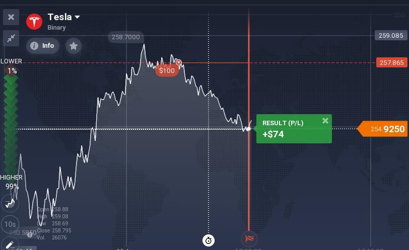
Then we tried the online trading platform called IQ option, by doing that, we invested
about 100$ (virtually), and since from our ARIMA model above we observed that the general
trend is going downwards, we we invested in the lower, which means that we predict that
the stock prices are going to decrease, and at the end of the day, we made about 74$
dollars, which means that our predictions are accurate and that in this trial, we made virtual
money out of the outcome of these ARIMA models
The figure below is the visual representation of the trial we did on IQ Option, we can
see the 100$ invested at the price of 257.865$ and the market closed at the price of
254.925$:38 Figure 15: visual representation of the trial on IQ Option
39

                                     Conclusion
       In this capstone project, we studied the index of the company TESLA Motors in order

to find mathematical models that we could use as a way to predict future values of the stock

prices. We chose this company because it is very interesting and unique since it

manufactures electrical cars , which makes it the future of the car industry since it is eco-

friendly and because sooner or later, natural resources will all be used. The model we chose

to use in order to predict the

        TESLA stock prices is the ARIMA model which stands for Auto Regressive Integrated

Moving Average, after using R Studio and ARIMA model on our data, we concluded that

most the predictions are close to the real values and that the percent difference between

the values is very small. We took into consideration all the news related to TESLA Motors

during that time in order to explain better the sudden fluctuations in the index, and since

the model cannot predict these kind of events, it will not be a hundred percent accurate, but

the results we got are close enough to build on.
40
Recommendations
After using the ARIMA model on the available data in order to forecast future stock
prices values, we conclude that it is a very simple and easy model to deal with, and it gives
very close predictions to real stock prices .As for the TESLA Motors investing matter, and
after taking into consideration recent event, I think it is best to wait for all these problems
that TESLA is facing to be solved and then invest in it, because as much as the index drops,
the overall yearly performance of the company keeps on increasing.41
References
[1]"R Time Series Analysis", www.tutorialspoint.com, 2019. [Online]. Available:
https://www.tutorialspoint.com/r/r_time_series_analysis.htm. [Accessed: 20- Mar- 2019].
[2]2019. [Online]. Available: https://www.nasdaq.com/symbol/tsla/interactive-
chart?timeframe=1y. [Accessed: 21- Apr- 2019].
[3]"Introduction to ARIMA models", People.duke.edu, 2019. [Online]. Available:
https://people.duke.edu/~rnau/411arim.htm. [Accessed: 21- Apr- 2019].
[4]S. Chatterjee, "Time Series Analysis Using ARIMA Model In R", DataScience+, 2019.
[Online]. Available: https://datascienceplus.com/time-series-analysis-using-arima-model-in-
r/. [Accessed: 21- Apr- 2019].
[5]"Arima function | R Documentation", Rdocumentation.org, 2019. [Online]. Available:
https://www.rdocumentation.org/packages/forecast/versions/8.5/topics/Arima. [Accessed:
21- Apr- 2019].
[6]"Lesson 3: Identifying and Estimating ARIMA models; Using ARIMA models to forecast
future values | STAT 510", Newonlinecourses.science.psu.edu, 2019. [Online]. Available:
https://newonlinecourses.science.psu.edu/stat510/node/49/. [Accessed: 21- Apr- 2019].
[7]"Yahoo is now part of Oath", Finance.yahoo.com, 2019. [Online]. Available:
https://finance.yahoo.com/news/average-car-prices-more-4-42 110000138.html?guccounter=1&guce_referrer=aHR0cHM6Ly9zZWFyY2gueWFob28uY29tL3 NlYXJjaD9mcj1tY2FmZWUmdHlwZT1FMjEwVVM5MTEwNUcwJnA9dGVzbGErbmV3cytqYW51 YXJ5KzIwMTk&guce_referrer_sig=AQAAAFCPTQwk_yU_c_jyEPVM- xBfqnY22SJWRJAZ9T6QaycRIsQLbxsSWTHfFTFh9JDILNjqRnf0SyPRAPdMu39pqwfCsAJaoFeNR eL9eRE6mM5Q8Wb5dCQPADATxdOYLKwb4nxVmmGjAE_F2erP4HqCX7p5qnBvGjdkQLyo8cR AsmI. [Accessed: 21- Apr- 2019]. [8]"Tesla, Inc. | History, Cars, Elon Musk, & Facts", Encyclopedia Britannica, 2019. [Online]. Available: https://www.britannica.com/topic/Tesla-Motors. [Accessed: 21- Apr- 2019]. [9]"The Making Of Tesla: Invention, Betrayal, And The Birth Of The Roadster", Business Insider, 2019. [Online]. Available: https://www.businessinsider.com/tesla-the-origin-story- 2014-10. [Accessed: 21- Apr- 2019]. [10]"Elon Musk's Tesla Roadster", En.wikipedia.org, 2019. [Online]. Available: https://en.wikipedia.org/wiki/Elon_Musk%27s_Tesla_Roadster. [Accessed: 21- Apr- 2019]. [11]"The history of Tesla and Elon Musk: A radical vision for the future of autos", Edition.cnn.com, 2019. [Online]. Available: https://edition.cnn.com/interactive/2019/03/business/tesla-history-timeline/index.html. [Accessed: 21- Apr- 2019]. [12]"Elon Musk", Biography, 2019. [Online]. Available: https://www.biography.com/business-figure/elon-musk. [Accessed: 21- Apr- 2019].
You can also read


