Situational awareness and forecasting for Norway - Situational awareness ...

Situational awareness and forecasting for Norway
 FHI COVID-19 modelling team

 Week 29, 11 August 2021

Highlights:
 • National epidemiological situation: According to our changepoint model, the estimated effec-
 tive reproduction number is 1.22 (median, 95% CI 0.96 - 1.51), on average since 15 July. Before
 that, from 15 June to 14 July, the estimated effective reproduction number was 0.89 (median, 95%
 CI 0.78-1.0). The estimated probability of the effective reproduction number to be above 1 since 15
 July is 94.5%. The SMC model estimates the 7-days averaged effective reproduction number during
 week 31 to be 1.19 (mean, 95% CI 0.97-1.47). In the SMC model, the estimated probability that
 the daily reproduction number one week ago was above 1 is 95%. The Epiestim model, which uses
 only test data, estimates the effective reproduction number as 1.17 (95% CI 1.11-1.24). Hence, all
 our national estimates of the recent transmissibility agree that the current reproduction number is
 around 1.2. There is a clear increase in recent cases, while the hospitalisation incidence is currently
 more stable. This is likely an effect of the vaccination, which protects more from severe disease.
 Since the start of the epidemic, we estimate that in total, 261.000 (95% CI 232.000- 287.000)
 individuals in Norway have been infected. The current estimate of the detection probability is
 around ∼58%, with a slight increasing tendency in recent weeks.
 • National forecasting: In one week, on 15 August, we estimate approximately 1095 new cases per
 day (median; 95% CI 488-1987), and a prevalence (total number of presently infected individuals
 in Norway) of 6143 (median; 95% CI 2938-10402). The number of COVID-19 patients in hospital
 (daily prevalence) on 15 August is estimated to be 50 (median 95% CI 27-76), and the number
 of patients on ventilator treatment is estimated to be 9 (median 95% CI 3-15); the corresponding
 predictions in three weeks (29 August) are 77 (95% CI 32 - 149) and 13 (95% CI 5 - 25). These
 predictions are, as usual, under the assumption that nothing is changed since today, so no changes
 in interventions, no changes in mobility and in people’s behaviour. In particular, we assume no
 changes in future hospitalisation risks, even though the hospitalisation risks are expected to decrease
 further in the short term because of vaccination. Incorporating this trend would have resulted in
 lower hospitalisation predictions. However, we have chosen not to do it, as we would have to make
 speculative and ad hoc guesses about how much the hospitalisation risks will decrease, as we cannot
 base the estimate on data yet. We get an excellent fit to the hospital incidence data. The model
 also captures the recent hospital prevalence data well.
 Long-term scenarios with vaccination suggest show that further reopening is possible during the
 coming months. Given the assumption of a high seasonality effect of 50%, the model expects some
 resurgence in the coming autumn and winter months. Because of vaccination, the probability that
 the surge capacity will exceed 500 ventilator beds is extremely low.

 • Regional epidemiological situation and forecasting: This week, there are large discrepancies
 between the regional estimates obtained from our changepoint model, the SMC model and the
 EpiEstim. There has been a recent increase in the number of imported cases, and testing has been
 irregular due to the vacation, which complicates the estimation of local reproduction numbers.
 We are currently working to understand better the sources of inconsistencies. Therefore, we don’t
 present any regional estimates this week but hope to produce results next week.

 1

• Telenor mobility data and the number of foreign visitors: Inter-municipality mobility lev-
 els are similar or higher in all counties, compared to that of the previous summer, one year ago.
 The number of foreign visitors to Norway has increased substantially in the the last couple of weeks,
 most noticeably visitors from Germany and Sweden. There is also an increase in visitors from the
 Netherlands. The rise in visitors is non-uniform across the country; for example the number of
 foreign roamers in Oslo is high but relatively constant.

 2

What this report contains:
This report presents results based on a mathematical infectious disease model describing the geographical
spread of COVID-19 in Norway. We use a metapopulation model (MPM) for situational awareness and
short-term forecasting and an individual-based model (IBM) for long-term predictions. The metapopu-
lation model (MPM) consists of three layers:
 • Population structure in each municipality.
 • Mobility data for inter-municipality movements (Telenor mobile phone data).

 • Infection transmission model (SEIR-model)
The MPM model produces estimates of the current epidemiological situation at the municipality, county
(fylke), and national levels, a forecast of the situation for the next three weeks. We run three different
models built on the same structure indicated above: (1) a national changepoint model, (2) a regional
changepoint model and (3) a national Sequential Monte Carlo model, named SMC model.

How we calibrate the model: The national changepoint model is fitted to Norwegian COVID-19
hospital incidence data from March 10 until yesterday and data on the laboratory-confirmed cases from
May 1 until yesterday. We do not use data before May 1, as the testing capacity and testing criteria
were significantly different in the early period.
Note that the the national changepoint model results are not a simple average or aggregation of the
results of the regional changepoint model because they use different data. The estimates and predictions
of the regional model are more uncertain than those of the national model. The regional model has more
parameters to be estimated and less data in each county; lack of data limits the number of changepoints we
can introduce in that model. In the regional changepoint model, each county has its own changepoints and
therefore a varying number of reproduction numbers. Counties where the data indicate more variability
have more changepoints.
The national SMC model is also calibrated to the hospitalisation incidence data (same data as described
above) and the laboratory-confirmed cases.

Telenor mobility data: The mobility data account for the changes in the movement patterns between
municipalities that have occurred since the start of the epidemic.

How you should interpret the results: The model is stochastic. To predict the probability of various
outcomes, we run the model multiple times to represent the inherent randomness.
We present the results in terms of mean values, 95% credibility intervals, medians, and interquartile
ranges. We emphasise that the credibility bands might be broader than what we display because there
are several sources of additional uncertainty which we currently do not fully explore Firstly, there are
uncertainties related to the natural history of SARS-CoV-2, including the importance of asymptomatic
and presymptomatic infection. Secondly, there are uncertainties associated with the hospitalisation
timing relative to symptom onset, the severity of the COVID-19 infections by age, and the duration
of hospitalisation and ventilator treatment in ICU. We continue to update the model assumptions and
parameters following new evidence and local data as they become available. A complete list of all updates
can be found at the end of this report.
Estimates of all reproductive numbers are uncertain, and we use their distribution to assure appropriate
uncertainty of our predictions. Uncertainties related to the model parameters imply that the reported
effective reproductive numbers should be interpreted with caution.

When we forecast beyond today, we use the most recent reproduction number for the whole future, if
not explicitly stated otherwise.
In this report, the term patient in ventilator treatment includes only those patients that require either
invasive mechanical ventilation or ECMO (Extracorporeal membrane oxygenation).

 3

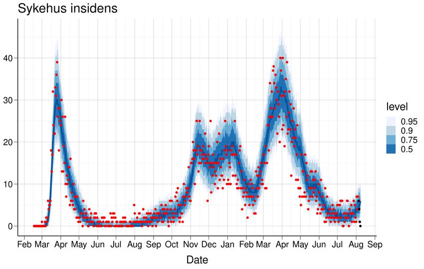
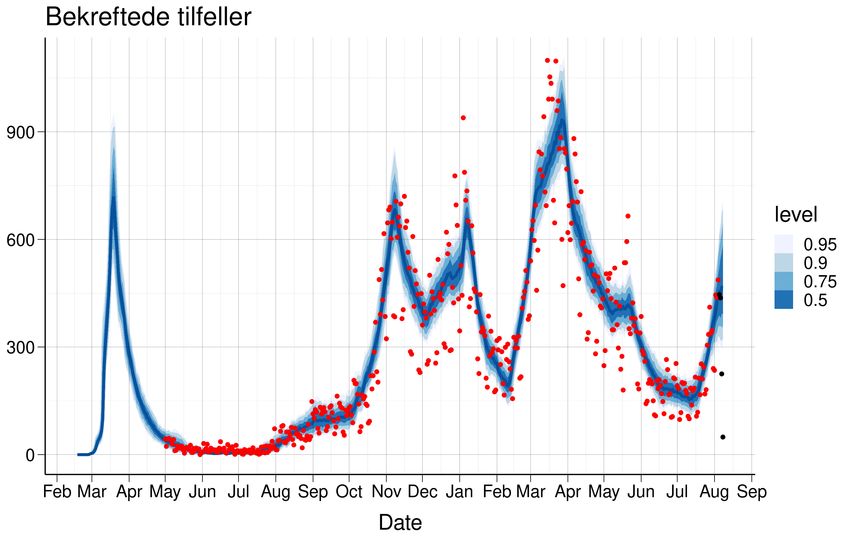
1 Estimated national reproduction numbers
Calibration of our national changepoint model to hospitalisation incidence data and test data leads to
the following estimates provided in table 1. Figure 1 shows the estimated daily number of COVID-19
patients admitted to hospital (1a) and the estimated daily number of laboratory-confirmed SARS-CoV-2
cases (1b), with blue medians and interquantile bands, which are compared to the actual true data,
provided in red. The uncertainty captures the uncertainty in the calibrated parameters in addition to
the stochastic elements of our model and the variability of other model parameters.

 Table 1: Calibration results

 Reff Period
 3.24/3.27(2.6-3.92) From Feb 17 to Mar 14
 0.55/0.53(0.41-0.63) From Mar 15 to Apr 19
 0.56/0.58(0.31-1.03) From Apr 20 to May 10
 0.48/0.5(0.07-0.91) From May 11 to Jun 30
 1.1/1.07(0.54-1.55) From Jul 01 to Jul 31
 1.05/1.08(0.76-1.42) From Aug 01 to Aug 31
 0.98/0.97(0.82-1.1) From Sep 01 to Sep 30
 1.24/1.24(1.04-1.42) From Oct 01 to Oct 25
 1.37/1.37(1.1-1.64) From Oct 26 to Nov 04
 0.82/0.82(0.76-0.87) From Nov 05 to Nov 30
 1.05/1.05(1-1.09) From Dec 01 to Jan 03
 0.63/0.63(0.52-0.73) From Jan 04 to Jan 21
 0.74/0.74(0.62-0.89) From Jan 22 to Feb 07
 1.45/1.45(1.32-1.56) From Feb 08 to Mar 01
 1.08/1.08(1.01-1.17) From Mar 02 to Mar 24
 0.79/0.79(0.73-0.84) From Mar 25 to Apr 15
 0.84/0.84(0.76-0.93) From Apr 16 to May 05
 1/1(0.88-1.12) From May 06 to May 19
 0.75/0.74(0.63-0.85) From May 20 to Jun 14
 0.89/0.89(0.78-1) From Jun 15 to Jul 14
 1.22/1.23(0.96-1.51) From Jul 15
 Median/Mean (95% credible intervals)

 4

(a) Hospital admissions (b) Test data

Figure 1: A comparison of true data (red) and predicted values (blue) for hospital admissions and test data. The last four
data points (black) are assumed to be affected by reporting delay. B) Comparison of our simulated number of positive cases,
with blue median and interquartile bands to the actual true number of positive cases, provided in red. The uncertainty
captures the uncertainty in the calibrated parameters, in addition to the stochastic elements of our model and the variability
of other model parameters. Note that we do not capture all the uncertainty in the test data–our blue bands are quite narrow.
This is likely because we calibrate our model parameters on a 7-days moving average window of test data, instead of daily.
This is done to avoid overfitting to random daily variation. Moving averages over 7 days are less variable than the daily
data.

 5

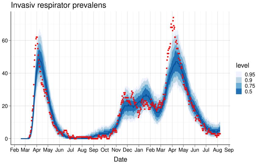
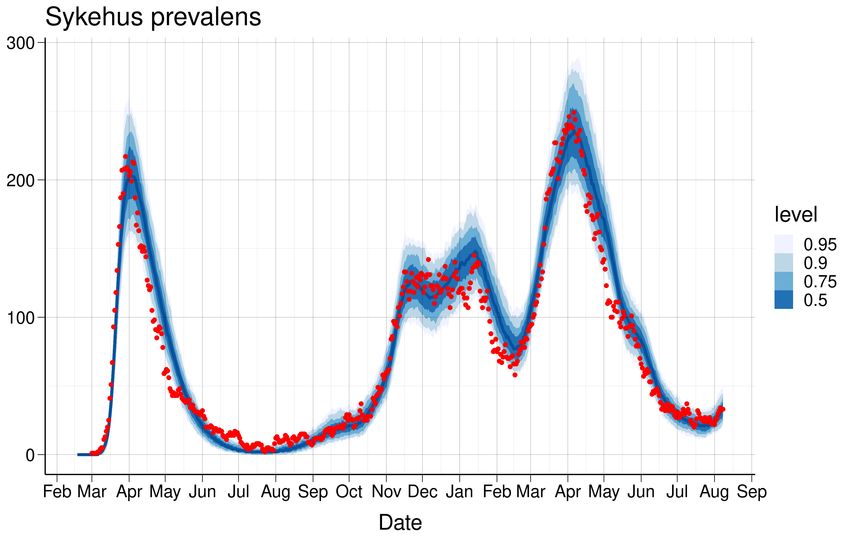
1.1 National SMC-model: Estimated daily reproduction numbers

 In figure 2, we show how our national model fits the national hospital prevalence data (2a) and the
daily number of patients receiving ventilator treatment (2b). Those data sources are not used to estimate
the parameters, and can therefore be seen as a validation of the model assumptions.

 (a) Hospital prevalence (b) Ventilator prevalence

Figure 2: A comparison of true data (red) and predicted values (blue) for hospital and respirator prevalence. Prevalence
data is based on NIPaR and may be different to the data from Helsedirektoratet.

1.1 National SMC-model: Estimated daily reproduction numbers
In the SMC-model, we allow for estimation of a different reproduction number for each day t. To reduce
spurious fluctuation, we report a 7-days moving average, R(t), representing the average reproduction
number for the whole week before day t. However, until March 8 we keep the reproduction number con-
stant. By assuming a time varying reproduction number R(t), we can detect changes without introducing
explicit changepoints. Thus, we can easier detect unexpected changes.

The SMC model uses the daily number of new admissions to hospital and the daily number of positive
and negative lab-confirmed tests, to estimate all its parameters. Because of the time between infection
and the possibility to be detected as positive by a test, and because if a delay in reporting tests, the data
contain information on the transmissibility until a week before the end of the data (today).

The parameters π0 and π1 related to the probability to detect a positive case by testing are estimated
off-line.

Figure 3 shows the SMC estimate of the 7-day-average daily reproduction number R(t) from the start of
the epidemic in Norway and until today. In the figure we plot the 95% credibility interval and quantiles
of the estimated posterior distribution of R(t).

 6

1.1 National SMC-model: Estimated daily reproduction numbers

Figure 3: R(t) estimates using a Sequential Monte Carlo approach calibrated to hospitalisation incidence and test data.
The large uncertainty during the last 7 days reflects the lack of available data due to the transmission delay, test delay,
time between symptoms onset and hospitalisation. The green band shows the 95% posterior credibility interval. As we use
test data only from 1 August, the credibility interval becomes more narrow thereafter.

 7

2 National estimate of cumulative (total) number of infections
The national changepoint model estimates the total number of infections and the symptomatic cases that
have occurred (Table 2).
Figure 4a shows the modelled expected daily incidence (blue) and the observed daily number of laboratory-
confirmed cases (red). When simulating the laboratory-confirmed cases, we also model the detection
probability for the infections (both symptomatic, presymptomatic and asymptomatic), Figure 4b. There
are two differences between this estimate of the detection probability and the previous one provided in
figure 4a. In figure 4b, we calibrate our model to the true number of positive cases, instead of using
the test data directly. Furthermore, in figure 4a we use a parametric model to estimate the detection
probability that depends on the true total number of tests performed.

 Table 2: Estimated cumulative number of infections, 2021-08-08

 Region Total No. confirmed Fraction reported Min. fraction
 Norway 260967 (231677; 287111) 138738 53% 48%
 Fraction reported=Number confirmed/number predicted; Minimal fraction reported=number confirmed/upper CI

(a) Number of laboratory-confirmed cases vs model-based esti-(b) Estimated detection probability for an infected case per cal-
mated number of new infected individuals endar day

 Figure 4

 8

3 National 3-week predictions: Prevalence, Incidence, Hospital
 beds and Ventilator beds
The national changepoint model estimates the prevalence and daily incidence of infected individuals
(asymptomatic, presymptomatic and symptomatic) for the next three weeks, aggregated to the whole
of Norway (table 3). In addition, the table shows projected national prevalence of hospitalised patients
(hospital beds) and prevalence of patients receiving ventilator treatment (ventilator beds). The projected
epidemic and healthcare burden are illustrated in figure 5.

 Table 3: Estimated national prevalence, incidence, hospital beds and ventilator beds. Median/Mean (CI)

 1 week prediction (Aug 15) 2 week prediction (Aug 22) 3 week prediction (Aug 29)
 Prevalence 6143/5625 (2938-10402) 7610/6629 (2885-15017) 9500/7996 (2861-21509)
 Daily incidence 1095/981 (488-1987) 1358/1164 (460-2893) 1697/1376 (445-4013)
 Hospital beds 50/50 (27-76) 63/57 (30-102) 77/70 (32-149)
 Ventilator beds 9/8 (3-15) 11/10 (3-19) 13/13 (5-25)

Figure 5: National 3 week predictions for incidence (top left), prevalence (bottom left), hospital beds (top right) and
ventilator beds (bottom right)

 9

4 National long-term scenarios with vaccination plans and fu-
 ture interventions: Infections, hospitalisations and ventilator
 treatments (updated 30th June 2021)
We present long-term scenarios from the individual-based model with vaccination including the vaccines
from Pfizer and Moderna, which are currently in the programme. In the model, the vaccines are offered
to everyone 18 years or older, as vaccination of 16- and 17-year olds has not yet been finally decided.
We present results with a seasonal effect of 50%. The seasonal effect is implemented by varying the
transmission rate in accordance with the mean daily temperature for Norway; hence, the transmission
rate varies by 50% between the coldest and warmest day during the year. We do not take into account
any potential increase in transmissibility or severity due to the introduction of the Delta variant, which
is believed to be gradually taking over in the coming months.
We use data from the Norwegian Immunisation Registry (SYSVAK) on the number of vaccinations car-
ried out up until 25th July 2021 1 . Vaccine deliveries in the future are based on the Norwegian Institute
of Public Health’s realistic (”nøktern”) scenario, last updated 18th June 2021. The roll-out accounts for
regional prioritisation with 45% additional vaccines to 24 municipalities: Oslo, Halden, Moss, Sarpsborg,
Fredrikstad, Drammen, Indre Østfold, Råde, Vestby, Nordre Follo, Ås, Frogn, Bærum, Asker, Rælingen,
Enebakk, Lørenskog, Lillestrøm, Nittedal, Gjerdrum, Ullensaker, Eidsvoll, Nannestad, and Lier.
We assume regional differences in the reproduction number between municipalities by estimating a scal-
ing factor for the reproduction number in each municipality. The scaling factor is calculated from the
local proportion of the population who has tested positive, compared to the national one. The initial
conditions in the municipalities are set following the results of the regional changepoint model. The
simulations until the end of March 2022 are based on the national reproduction number (Table 1) from
the national changepoint model, adjusted per municipality as described above. The long-term scenario
results are based on 100 simulations and account for stochasticity within the IBM model; however, the
uncertainty in the changepoint models is not accounted for, neither the uncertainty in the estimated
reproduction number, nor the uncertainty in the initial conditions.

4.1 Scenarios and how to interpret them
The future course of the epidemic will depend on the national and local control measures that the
authorities impose to curb the transmission in the current and future waves of the epidemic. In addition,
the epidemiological situation is highly uncertain. Therefore, the scenarios shown are not predictions but
are the modelled outcomes of a specific set of assumptions about the epidemic and how the government
and local authorities are assumed to act. We present results from two different scenarios:
Constant Scenario: In this scenario, we assume that the national vaccine roll-out continues as planned
and that the current epidemiological situation remains unchanged. In this scenario, the epidemic will
evolve according to the current reproduction number, and the government will make no changes to
the current interventions. We use three different assumptions for the national reproduction number:
R ∈ [1.1, 1.2, 1.3]. This is done to account for the spread in the estimates of R from the national
changepoint model (1.22), SMC model (1.19) and EpiEstim model (1.17).
Controlled Scenario: In this alternative scenario, we assume that the national vaccine roll-out will
continue as planned. We assume the national reproduction number of R = 1.2 on 8th August. However,
the government chooses to actively control the reopening of the society in relation to the prevalence of
hospital admissions at a given time. We set an upper threshold of 200 admitted patients nationally. If
this threshold is reached, contact-reducing measures are triggered. In the model, we assume that the
contact-reducing measures will reduce the reproduction number to 0.8. We also include a lower threshold
of 50 hospital admissions nationally. If this threshold is reached, a lowering of contact-reducing measures
is triggered. In this case, increase the reproduction number in the model to 1.2. We also have a middle
threshold of 125 hospital admissions nationally. If the prevalence of hospital admissions is between 50
 1 Weuse a two-week period from 26th July to 8th August to initialize the model – results here are shown starting from
26th July.

 10

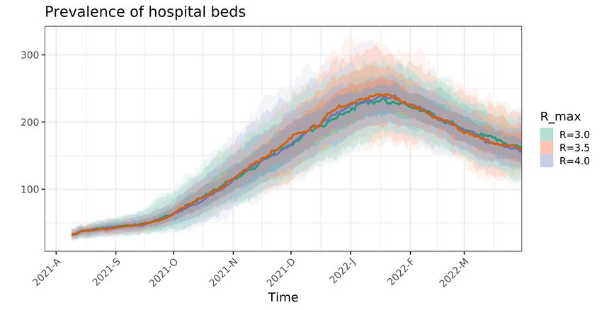
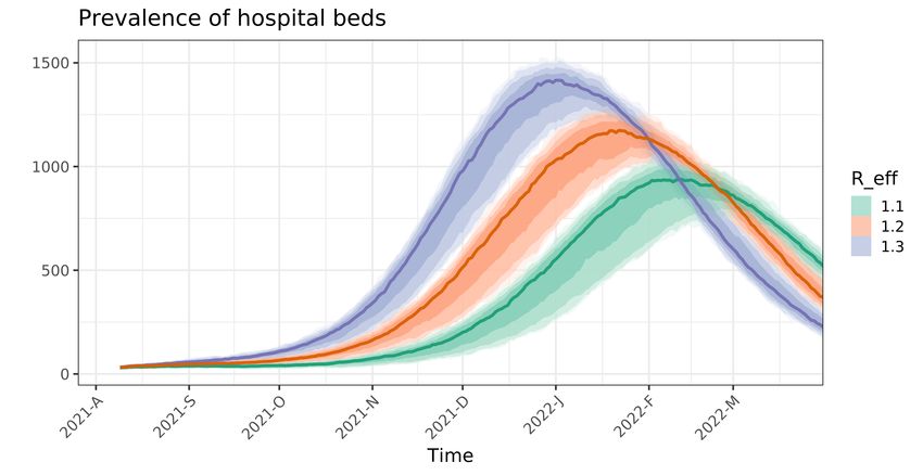
4.2 Constant Scenario

and 125, we update the reproduction number to 1.05; while if the prevalence of hospital admissions is
between 125 and 200, we update the reproduction number to 1.0. The number of hospital admissions is
evaluated every two weeks to simulate a gradual reopening or closing, and if needed, the reproduction
number is changed. We implement the corrections at a regional level by calculating regional threshold
values per inhabitants based on the three national threshold levels above. Note that these thresholds
which trigger reopening and contact-reducing measures in the simulations have been arbitrarily chosen
as an illustration of a controlled scenario, and we could also have used different numbers.
In a controlled scenario, we need to make assumptions on how much we can reopen compared to the
current level and what contact rate that corresponds to ”normal” social contact without intervention
measures. We enforce a maximum reproduction number for each municipality within the model – the
model is not allowed to increase the contact rate above this threshold, even though hospital prevalence
allows. The threshold is estimated based on an assumed basic reproduction number for the epidemic of
R0 ∈ [2, 2.33, 2.66]. The R0 is multiplied by a factor of 1.5 to take into account the higher transmissibility
of the B.1.1.7 strain that is dominating in Norway, bringing the range of R values used for our controlled
scenarios to R ∈ [3, 3.5, 4].
Both scenarios are made given some simplifying assumptions:

 • The vaccine uptake is assumed to be 90% in all age groups 18 years old and above and we assume
 full adherence to the vaccination schedule.
 • We use modest assumptions on the vaccine efficacy (VE). For the vector vaccines: VE asymp (1.
 and 2. dose) 22%; VE symp (1. and 2. dose) 70%; VE sev (1. and 2. dose) 80%. For the mRNA
 vaccines: VE asymp (1. and 2. dose) 55%, 77%; VE symp (1. and 2. dose) 71%, 91%; VE sev (1.
 and 2. dose) 78%, 94%. People who are vaccinated and get infected are assumed to transmit 65%
 less than those who are not vaccinated.
 • We assume the following total number of imported cases per month (the imported cases are then
 evenly distributed over the days of the month): June 1125; July 800; August 500; September 205;
 October 152; November 91; December 72; January through March 2022 100.

 • We assume a twelve-week interval between the first and second mRNA vaccine doses.
 • No waning immunity after infection or vaccination is assumed.
 • We assume that the vaccines are effective against all circulating variants.

More information about the IBM can be found in the reports Folkehelseinstituttets foreløpige anbefalinger
om vaksinasjon mot covid-19 og om prioritering av covid-19-vaksiner, versjon 2 15. desember and Model-
leringsrapport, delleveranse Oppdrag 8: Effekt av regional prioritering av covid-19 vaksiner til Oslo eller
OsloViken samt vaksinenes effekt på transmisjon for epidemiens videre utvikling, available online at http:
//www.fhi.no. The order of priority for age and risk groups can be found at https://www.fhi.no/en/
id/vaccines/coronavirus-immunisation-programme/who-will-get-coronavirus-vaccine-first/.
A detailed description of the controlled scenario’s assumptions is provided in recent modelling reports,
to be published shortly.

4.2 Constant Scenario
We present scenarios until the end of March 2022 from our IBM with vaccination, showing expected
prevalence (Figure 6a), hospital beds (Figure 6b) and ventilator beds (Figure 6c).

Depending on the assumed epidemiological situation (R ranging from 0.6 to 1) and assuming a seasonal
effect of 50%, the epidemic exhibits a peak in late June in the case of R = 1, else a steady decline, as
seen in Figure 6. None of the scenarios exceed a surge capacity need of 500 ICU ventilator beds (Table
4).

 11

4.2 Constant Scenario

 Table 4: Estimated total infections, admissions and ventilator treatments until 31st March 2022

 Reproduction number
 Total 1.1 1.2 1.3
 Infections 873752 (789690-957814) 1102862 (1044195-1161529) 1269721 (1225070-1314372)
 Hospitalisations 10880 (9638-12123) 14453 (13497-15410) 17163 (16412-17914)
Ventilator treatments 1410 (1230-1591) 1903 (1771-2034) 2267 (2158-2376)

 (a)

 (b)

 12

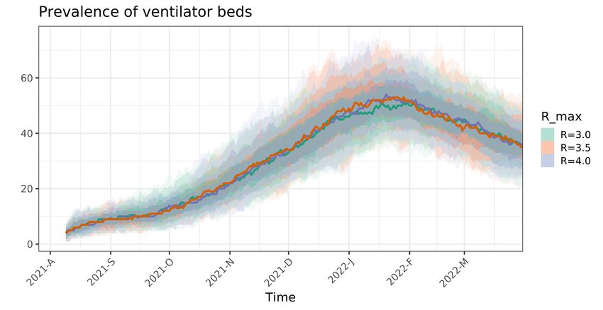
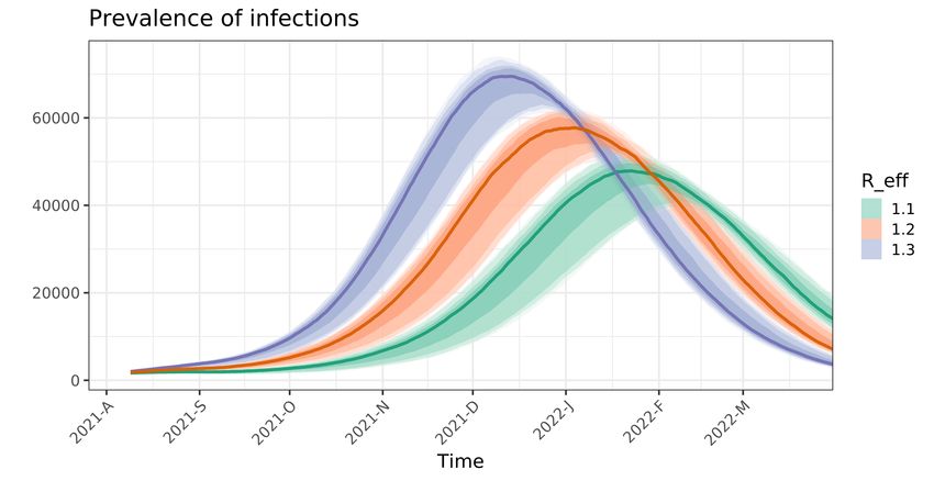
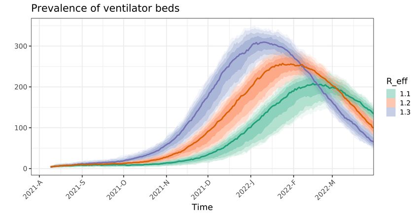
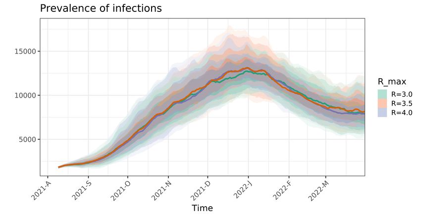
4.3 Controlled Scenario

4.3 Controlled Scenario
We next present long-term projections using the controlled scenarios described above, showing expected
prevalence (Figure 7a), hospital beds (Figure 7b) and ventilator beds (Figure 7c).
Figure 8 shows at a national level the relative average contact rate compared to an open society with
“normal” social interaction. To estimate the level of contact corresponding to a fully open community, we
first calculate the early transmission rate in each region, corresponding to the period before the lockdown
in March 2020, from the estimated basic reproduction number, R0 . We use three different assumptions
for R0 to illustrate the uncertainty.
The transmission rate, the so-called beta parameter, is the product of the contact rate multiplied with the
probability of transmission given contact. We can think of the transmission rate as an effective contact
rate, relevant to the spread of the SARS-CoV-2 virus.
Note that the reopening is simulated locally and that the degree of reopening may differ in the various
regions of the country.

 Table 5: Estimated total number of infections, hospitalisations and ventilator treatments until 31st March 2022

 Maximum reproduction number
 Total 3 3.5 4
 Infections 374869 (342881-406858) 380067 (346299-413834) 375095 (342469-407721)
 Hospitalisations 4375 (3969-4781) 4413 (3990-4837) 4368 (3950-4787)
 Ventilator treatm. 561 (505-617). 561 (507-615) 556 (497-616)

Table 5 shows that, in a controlled scenario with hospital admissions as steering parameter, there is an
increasing trend in the expected infections and admissions when the maximum reproduction number (i.e.
1.5R0 ) increases. Figure 8 indicates that a continuation of the gradual reopening is possible the coming
months. In the scenarios assuming different maximum reproduction number (e.g. 3, 3.5 and 4), full
reopening is possible in August and September; however, the model suggests that it will be necessary to
implement measures to limit the contact during the autumn and winter; and possibly to reopen again in
spring 2022. The reduced contact rate in the last part (January to March) is likely due to time-delay in
the response. The hospital level is delayed with respect to the infection incidence curve (Figure 7).

 13

4.3 Controlled Scenario

 (a)

 (b)

 (c)

Figure 7: Long-term predictions from the controlled scenario, for prevalence (a),hospital beds (b) and ventilator
beds (c). Each color shows the scenario of one maximum reproduction number, 3, 3.5 and 4.

 14

4.3 Controlled Scenario

Figure 8: Relative average national contact rate compared to a fully open society using a reopening factor to determine
the maximum level of reopening in the controlled scenario. Each line represents one reopening factor and is normalized
by its own maximum contact rate. Simulations are made with vaccines from Pfizer and Moderna, assuming the modest
(”Nøktern”) vaccine delivery schedule. The contact rate is population-weighted average in all municipalities, updated every
two weeks to simulate gradual reopening by evaluating the number of hospital admissions.

 15

5 14-day trend analysis of confirmed cases and hospitalisations
 by county
To estimate recent trends in hospitalisation and number of positive tests, we present results in table 6
based on a negative binomial regression where we account for weekend effects. We exclude the last three
days to avoid problems of reporting delay and fit the model using data from 17 days to 3 days before the
current date. We fit a separate trend model for confirmed cases and for hospital incidence. We only fit
a trend model if there has been more than 5 cases or hospitalisations in the 14-day period.

 Table 6: Trend analysis for the last 14 days

 Average daily increase last 14 days Doubling Time (days)
 County Hospitalisations Cases Hospitalisations Cases
 Agder Not enough data -0.6 ( -4.8, 3.7) % Not enough data -107.3 ( -14.1, 19.2)
 Innlandet Not enough data 11.7 ( 6.9, 16.8) % Not enough data 6.3 ( 10.4, 4.5)
 Møre og Romsdal Not enough data -5 ( -11, 1.6) % Not enough data -13.6 ( -5.9, 44.9)
 Nordland Not enough data 4.1 ( -3.5, 12.4) % Not enough data 17.3 ( -19.3, 5.9)
 Norge 1.4 ( -6, 9.4) % 3.8 ( 2.9, 4.8) % 49.3 ( -11.3, 7.7) 18.4 ( 24.1, 14.9)
 Oslo Not enough data 6.2 ( 4.3, 8.1) % Not enough data 11.5 ( 16.4, 8.9)
 Rogaland Not enough data 4.2 ( 0.8, 7.6) % Not enough data 17 ( 82.4, 9.5)
 Troms og Finnmark Not enough data -0.3 ( -5.1, 4.8) % Not enough data -255.6 ( -13.2, 14.8)
 Trøndelag Not enough data 6.3 ( 2.3, 10.5) % Not enough data 11.4 ( 30.1, 7)
 Vestfold og Telemark Not enough data 0.7 ( -2.5, 4.1) % Not enough data 95 ( -27.5, 17.4)
 Vestland Not enough data 6.5 ( 5, 8.2) % Not enough data 10.9 ( 14.3, 8.8)
 Viken Not enough data 3.2 ( 0.7, 5.8) % Not enough data 21.8 ( 94, 12.3)

 16

6 Mobility
Number of trips out from each municipality during each day is based on Telenor mobility data. We
observed a large reduction in inter-municipality mobility in March 2020 (with minimum reached on
Tuesday 17 March 2020), and thereafter we see an increasing trend in the mobility lasting until vacation
time in July 2020. The changes in mobility in July 2020 coincides with the three-week ”fellesferie” in
Norway, and during August the mobility resumes approximately the same levels as pre-vacation time.
There is however a significant regional variation.
The reference level is set to 100 on March 2nd 2020 for all the figures in this section, and we plot the
seven-day, moving average of the daily mobility. Figure 9 shows an overview of the mobility since March
2020 for the largest municipalities in each county, and Figure 10 shows the total mobility out from all
municipalities in each county, including Oslo. Figure 11 and 12, zooms in on mobility from April 19
2021, for municipalities and counties, respectively.

Figure 9: Mobility for selected municipalities since March 2020: Nationally (Norge), Stavanger (1103), Ålesund (1507),
Bodø (1804), Bærum (3024), Ringsaker (3411), Sandefjord (3804), Kristiansand (4204), Bergen (4601), Trondheim (5001),
Tromsø (5401).

 17

Figure 10: Mobility for fylker since March 2020: Oslo (03), Rogaland (11), Møre og Romsdal (15), Nordland (18), Viken
(30), Innlandet (34), Vestfold og Telemark (38), Agder (42), Vestland (46), Trøndelag (50), Troms og Finmark (54).

 18

Figure 11: Zoom: Mobility from April 19, 2021 and onwards: Nationally (Norge), Stavanger (1103), Ålesund (1507),
Bodø (1804), Bærum (3024), Ringsaker (3411), Sandefjord (3804), Kristiansand (4204), Bergen (4601), Trondheim (5001),
Tromsø (5401).

 19

Figure 12: Zoom: Mobility from April 19, 2021 and onwards, per fylker: Oslo (03), Rogaland (11), Møre og Romsdal (15),
Nordland (18), Viken (30), Innlandet (34), Vestfold og Telemark (38), Agder (42), Vestland (46), Trøndelag (50), Troms
og Finnmark (54).

 20

27 28 29 30 31
 Norge 100.0 101.2 99.6 99.9 99.9
 Stavanger 81.7 77.1 74.6 72.9 71.4
 Ålesund 102.5 104.6 108.2 105.3 105.2
 Bodø 126.6 141.1 146.9 138.5 130.4
 Bærum 67.0 60.8 49.5 43.3 41.9
 Ringsaker 95.0 94.0 91.4 91.3 92.2
 Sandefjord 97.2 99.6 101.1 109.2 109.7
 Kristiansand 113.5 120.2 129.3 136.5 135.0
 Bergen 92.5 89.3 83.6 76.7 74.9
 Trondheim 104.8 110.3 105.5 99.7 96.8
 Tromsø 134.6 144.6 143.6 135.1 135.7

 Table 7: Municipalities

 27 28 29 30 31
 Oslo 67.6 64.2 55.4 50.2 48.8
 Rogaland 88.8 83.3 81.3 78.4 76.9
 Møre og Romsdal 114.6 121.8 125.7 125.7 132.1
 Nordland 161.1 186.5 206.8 194.9 180.4
 Viken 86.0 83.5 77.4 75.3 74.1
 Innlandet 119.0 122.4 123.8 133.1 136.8
 Vestfold og Telemark 108.5 111.4 112.8 122.2 123.0
 Agder 121.0 126.7 138.2 150.9 151.3
 Vestlandet 107.9 110.0 108.0 109.5 114.9
 Trøndelag 119.2 128.2 126.1 123.4 122.5
 Troms og Finnmark 134.4 143.1 150.0 144.8 138.3

 Table 8: Counties

Weekly mobility for Norway and selected municipalities is displayed in Table 7 and mobility for counties
is displayed in Table 8. The percentages in the tables are to be interpreted towards the reference level
of 100 for week 10 in March 2020. The color-coding encodes the following: ’Green’ monotonic decrease
in mobility, ’Yellow’ almost monotonic decrease or flat mobility trend, ’Red’ increasing mobility.

 21

6.1 Foreign roamers on Telenor’s network in Norway

6.1 Foreign roamers on Telenor’s network in Norway
An analysis of foreign roamers in Norway from January 2020 has been carried out, to better understand
the potential virus importation. In Figure 13 the total number of roamers per day per county are
displayed. We can see an approximate 40% drop in the number of visiting roamers after the lock-down
in March 2020. The number of visiting roamers recover during the Summer of 2020, and there is a spike
of visitors in August followed by a drop again. During October and November 2020 the levels of visiting,
foreign roamers to Norway have reached quite high levels, just 10% short of the all-year high for 2020,
and Oslo and Viken have seen big increases in visitors. There is a reduction in visitors during Christmas,
and in January 2021 we see an increasing trend again.
 Figure 14 shows the levels of roamers from the following countries: Poland, Lithuania, Sweden,
Netherlands, Denmark, Latvia, Germany, Spain, Finland and the rest of the world. These levels represent
the total number of foreign, visiting roamers from each of the countries per day in Norway, since April
19 2021.

Figure 13: The total number of foreign roamers in Norway broken down on different fylker: Oslo (3), Rogaland (11),
Møre og Romsdal (15), Nordland (18), Viken (30), Innlandet (34), Vestfold og Telemark (38), Agder (42), Vestland (46),
Trøndelag (50), Troms og Finnmark (54).

 22

6.1 Foreign roamers on Telenor’s network in Norway

Figure 14: National overview of total number of foreign, visiting roamers from Poland, Lithuania, Sweden, Netherlands,
Denmark, Latvia, Germany, Spain, Finland and the rest of the world.

 23

6.2 Foreign roamers per county (fylke) in Norway

6.2 Foreign roamers per county (fylke) in Norway

 24

6.2 Foreign roamers per county (fylke) in Norway

 25

7 Methods
7.1 Model
We use a metapopulation model to simulate the spread of COVID-19 in Norway in space and time. The
model consists of three layers: the population structure in each municipality, information about how
people move between different municipalities, and local transmission within each municipality. In this
way, the model can simulate the spread of COVID-19 within each municipality, and how the virus is
transported around in Norway.

7.1.1 Transmission model
We use an SEIR (Susceptible-Exposed-Infected-Recovered) model without age structure to simulate the
local transmission within each area. Mixing between individuals within each area is assumed to be ran-
dom. Demographic changes due to births, immigration, emigration and deaths are not considered. The
model distinguishes between asymptomatic and symptomatic infection, and we consider presymptomatic
infectiousness among those who develop symptomatic infection. In total, the model consists of 6 dis-
ease states: Susceptible (S), Exposed, infected, but not infectious (E1 ), Presymptomatic infected (E2 ),
Symptomatic infected (I), Asymptomatic infected (Ia ), and Recovered, either immune or dead (R). A
schematic overview of the model is shown in figure 17.

 Susceptible, S
 / 
 $" " / 
 () ) / 

 Exposed, not
 infectious, no
 symptoms, E1
 , (1 − " ) , "
 Exposed,
 Infectious
 presymptomatic,
 asymptomatic, "
 infectious, E2

 )

 γ
 Infectious,
 symptomatic, I
 γ
 Recovered, R

 Figure 17: Schematic overview of the model.

7.2 Movements between municipalities:
We use 6-hourly mobility matrices from Telenor to capture the movements between municipalities. The
matrices are scaled according to the overall Telenor market share in Norway, estimated to be 48%. Since
week 8, we use the actual daily mobility matrices to simulate the past. In this way, alterations in the
mobility pattern will be incorporated in our model predictions. To predict future movements, we use the

 26

7.3 Healthcare utilisation

latest weekday measured by Telenor, regularised to be balanced in total in- and outgoing flow for each
municipality.

7.3 Healthcare utilisation
Based on the estimated daily incidence data from the model and the population age structure in each
municipality, we calculated the hospitalisation using a weighted average. We correct these probabilities
by a factor which represents the over or under representation of each age group among the lab confirmed
positive cases. The hospitalisation is assumed to be delayed relative to the symptom onset. We calculate
the number of patients admitted to ventilator treatment from the patients in hospital using age-adjusted
probabilities and an assumed delay.

7.4 Seeding
At the start of each simulation, we locate 5.367.580 people in the municipalities of Norway according to
data from SSB per January 1. 2020. All confirmed Norwegian imported cases with information about
residence municipality and test dates are used to seed the model, using the data available until yesterday.
For each case, we add an additional random number of infectious individuals, in the same area and on
the same day, to account for asymptomatic imported cases who were not tested or otherwise missed. We
denote this by the amplification factor.

7.5 Calibration
Estimation of the parameters of the model: the reproduction numbers, the amplification factor for the
imported cases, the parameters of the detection probability and the delay between incidence and test,
is done using Sequential Monte Carlo Approximate Bayesian Computation (SMC-ABC), as described
in Engebretsen et al. (2020): https://royalsocietypublishing.org/doi/10.1098/rsif.2019.0809, where the
algorithm can be found in the supplement.
 The idea behind ABC is to try out different parameter sets, simulate using these, then compare how
much the simulations deviate from the observations in terms of summary statistics. We thus test millions
of combinations of the different reproductive numbers, the amplification factor, and the parameters for
the positive tests, to determine the ones that lead to the best fits to the true number of hospitalised
individuals, from March 10 2020 until the last available data point, and the laboratory-confirmed COVID-
19 cases from May 1 until the latest available data point.
 In the ABC procedure we thus use two summary statistics, one is the distance between the simulated
hospitalisation incidence and the observed incidence, and the other is the distance between the observed
number of laboratory-confirmed cases and the simulated ones. As the two summary statistics are not on
the same scale, we use two separate tolerances in the ABC-procedure, ensuring that we get a good fit to
both data sources.

7.5.1 Calibration to hospitalisation data
In order to calibrate to the hospitalisation data, we need to simulate hospital incidence. The details on
how we simulate hospitalisations are described in Section 7.3, using the parameters provided in Section
8, which are estimated from individual-level Norwegian data, and updated regularly. As our distance
measure, we calculate the squared distance over each time point and each county.

7.5.2 Calibration to test data
We include the laboratory-confirmed cases in the calibration procedure, as these contain additional
information about the transmissibility, and the delay between transmission and testing is shorter than
the delay between transmission and hospitalisation. Therefore, we simulate also the number of detected
positive cases in our model. We assume that the number of detected positive cases can be modelled as a
binomial process of the simulated daily total incidence of symptomatic and asymptomatic cases, with a

 27

7.6 Specifications for the national changepoint model

success probability πt , which changes every day. We also assume a delay d between the day of test and
the day of transmission.
 The data on the number of positive cases are more difficult to use, as the test criteria and capacity
have changed multiple times. We take into account these changes by using the total number of tests
performed on each day, as a good proxy of capacity and testing criteria. Moreover, we choose not to
calibrate to the test data before May 1, because the test criteria and capacity were so different in the
early period. The detection probability is modelled as

 πt = exp (π0 + π1 · kt )/(1 + exp(π0 + π1 · kt )),

where kt is the number of tests actually performed on day t, and π0 and π1 are two parameters that we
estimate, assuming positivity of π1 . We also estimate the delay d. We choose to use a 7-days backwards
moving average for the covariate kt . To calculate the distance between the observed number of positive
tests and the simulated ones we also use a 7-days backwards moving average. We do this to take into
account potential day-of-the-week-effects. For example, it could well be that the testing criteria are
different on weekends and weekdays. However, using instead the number of tests and calibrating on a
daily basis would lead to a larger day-to-day variance. This is likely why we find that the uncertainty
in the simulated positive cases seems somewhat too low, and that we do not capture all the variance
in the daily test data. Moreover, the binomial assumption could be too simple, and a beta-binomial
distribution would allow more variance. A limitation of our current model for the detection probability,
is that we only capture the changes in the test criteria that are captured in the total number of tests
performed.

7.6 Specifications for the national changepoint model
In the national changepoint model, we assume a first reproduction number R0 until March 14, a sec-
ond reproduction number R1 until April 19, a third reproduction number R2 until May 10, a fourth
reproduction number R3 until June 30, R4 until July 31, R5 until August 31, R6 from September 1
until September 30, R7 from October 1 until October 26, R8 until November 4, R9 from November 5th
until November 30th, R10 from December 1st until January 4, a twelfth reproduction number R11 from
January 4 until January 21, a thirteenth reproduction number from January 22 to February 7 and a
fourteenth reproduction number from February 8. This last reproduction number is used for the future.
The changepoints follow the changes in restrictions introduced. In the calibration procedure, we obtain
200 parameter sets that we use to represent the distributions of parameters.
 After we have obtained the estimated parameters, we run the model with these 200 parameter sets
again, from the beginning until today, plus three weeks into the future (or for an additional year). In
this way, we obtain different trajectories of the future, allowing us to investigate different scenarios, with
corresponding uncertainty.

7.7 Specifications for the regional changepoint model
In the regional changepoint model, each county has its own reproduction numbers, assumed constant in
different periods, just like the national changepoint model. As there are more parameters in the regional
changepoint model, we obtain 1000 parameter sets in the ABC-SMC.
 Calibrating regional reproduction numbers is a more difficult estimation problem than calibrating
national reproduction numbers, as we have a lot more parameters, and in addition less data in each
county. Therefore, we cannot include the same amount of changepoints in the regional model as we can
for the national model.
 After we have obtained the estimated parameters, we run the model with these 1000 parameter sets
again, from the beginning until today, plus three weeks into the future (or for an additional year). In
this way, we obtain different trajectories of the future, allowing us to investigate different scenarios, with
corresponding uncertainty.

 28

8 Parameters used today
Figures 18 to 23 indicate which assumptions we make in our regional model, related to hospitalisation.
We obtained data from the Norwegian Pandemiregister. These estimates will be regularly updated, on
the basis of new data.

 p = 0.85 Ward

 Neg binomial
 Mean = 6.11
 Onset of symptoms Hospital days size = 2.11 Discharged

 back in ward
 Neg. binomial time Neg bi-
 mean 8.72 days Ward ICU Ward
 p = 0.15 nomial, mean
 size = 3.65 14.61 days, size
 Neg. binomial
 Neg. binomial 2.00
 mean 15.93
 mean 1.83 days
 days, size =
 size= 1.46
 2.03

 Figure 18: Hospital assumptions and parameters used before 1 June 2020

 p = 0.90 Ward

 Neg binomial
 Mean = 5.45
 Onset of symptoms Hospital days size = 1.71 Discharged

 back in ward
 Neg. binomial time Neg. bi-
 mean 7.37 days Ward ICU Ward
 p = 0.10 nomial, mean
 size = 3.07 12.24 days, size
 Neg. binomial
 Neg. binomial 1.67
 mean 12.76
 mean 2.52 days
 days, size =
 size = 1.55
 1.16

 Figure 19: Hospital assumptions and parameters used between 1 June 2020 and 1 January 2021

 p = 0.84 Ward

 Neg binomial
 Mean = 6.09
 Onset of symptoms Hospital days size = 2.61 Discharged

 Neg. binomial back in ward
 mean 6.09 days Ward ICU Ward time Neg. bino-
 p = 0.16 mial, mean 8.71
 size = 2.61
 Neg. binomial days, size 2.50
 Neg. binomial
 mean 12.74
 mean 2.83 days
 days, size =
 size = 1.49
 1.29

Figure 20: Hospital assumptions and parameters used between 1 January 2021 and 1 March 2021 for those living in Oslo

 29

p = 0.87 Ward

 Neg binomial
 Mean = 5.74
 Onset of symptoms Hospital days size = 1.71 Discharged

 back in ward
 Neg. binomial time Neg. bi-
 mean 7.94 days Ward ICU Ward
 p = 0.13 nomial, mean
 size = 4.65 10.18 days, size
 Neg. binomial
 Neg. binomial 1.97
 mean 14.76
 mean 3.91 days
 days, size =
 size = 1.36
 1.76

Figure 21: Hospital assumptions and parameters used between 1 January 2021 and 1 March 2021 for those not living in
Oslo

 p = 0.84 Ward

 Neg binomial
 Mean = 5.35
 Onset of symptoms Hospital days size = 1.96 Discharged

 Neg. binomial back in ward
 mean 5.35 days Ward ICU Ward time Neg. bino-
 p = 0.16 mial, mean 8.71
 size = 1.96
 Neg. binomial days, size 2.50
 Neg. binomial
 mean 12.73
 mean 2.83 days
 days, size =
 size = 1.49
 1.29

 Figure 22: Hospital assumptions and parameters used from 1 March 2021 for those living in Oslo

 p = 0.87 Ward

 Neg binomial
 Mean = 5.66
 Onset of symptoms Hospital days size = 2.00 Discharged

 back in ward
 Neg. binomial time Neg. bi-
 mean 8.23 days Ward ICU Ward
 p = 0.13 nomial, mean
 size = 7.73 10.18 days, size
 Neg. binomial
 Neg. binomial 1.97
 mean 14.76
 mean 3.91 days
 days, size =
 size = 1.36
 1.76

 Figure 23: Hospital assumptions and parameters used from 1 March 2021 for those not living in Oslo

 30

Table 9: Estimated parameters

 Min. 1st Qu. Median Mean 3rd Qu. Max. Period
 R0s 2.519 3.009 3.243 3.273 3.558 4.097 Until March 14
 R1s 0.315 0.481 0.547 0.534 0.584 0.65 From 15 March to 19 April
 R2s 0.185 0.439 0.563 0.577 0.689 1.226 From 20 April to 10 May
 R3s 0.003 0.343 0.481 0.496 0.659 1.12 From 11 May to 30 June
 R4s 0.275 0.882 1.1 1.072 1.278 1.713 From 01 July to 31 July
 R5s 0.702 0.946 1.052 1.08 1.209 1.438 From 01 August to 31 August
 R6s 0.713 0.919 0.976 0.969 1.022 1.192 From 01 September to 30 September
 R7s 0.972 1.177 1.243 1.242 1.305 1.499 From 01 October to 25 October
 R8s 0.872 1.281 1.375 1.37 1.469 1.684 From 26 October to 04 November
 R9s 0.748 0.797 0.816 0.818 0.839 0.88 From 05 November to 30 November
R10s 0.984 1.03 1.048 1.047 1.063 1.106 From 01 December to 03 January
R11s 0.47 0.585 0.625 0.628 0.671 0.774 From 04 January to 21 January
R12s 0.542 0.68 0.739 0.737 0.783 0.936 From 22 January to 07 February
R13s 1.255 1.414 1.449 1.448 1.485 1.599 From 08 February to 01 March
R14s 0.97 1.045 1.081 1.08 1.113 1.192 From 02 March to 24 March
R15s 0.716 0.775 0.793 0.791 0.809 0.857 From 25 March to 15 April
R16s 0.728 0.808 0.836 0.841 0.872 0.994 From 16 April to 05 May
R17s 0.824 0.953 0.996 0.997 1.043 1.216 From 06 May to 19 May
R18s 0.542 0.706 0.746 0.745 0.786 0.861 From 20 May to 14 June
R19s 0.749 0.851 0.887 0.891 0.931 1.102 From 15 June to 14 July
R20s 0.895 1.122 1.225 1.227 1.322 1.541 From 15 July
AMPs 1.007 1.506 1.938 1.962 2.337 3.539 -
 π0 -0.523 -0.032 0.077 0.075 0.2 0.451 -
 π1 1.4e-06 1.6e-05 2.3e-05 2.4e-05 3.0e-05 6.1e-05 -
delays 0 1 2 2.09 3 4 -

 31

Frequency Frequency Frequency Frequency Frequency Frequency
 0 20 40 0 20 60 0 20 40 0 20 40 0 20 40 0 20 40

 2.5

 0.6

 1.0
 0.5

 R8
 R4
 R0

 R20
 R16
 R12
 0.8
 3.5

 1.4
 0.8 1.2 1.6
 1.5

 1.0

 0.75 0.90 1.05
 Frequency Frequency Frequency Frequency Frequency
 0 20 40 0 20 50 0 20 40 0 20 40 0 20 50
 0.3

 0.75

 0.9
 1.3
 0.8

 R9
 R5
 R1
 0.5

 R17
 R13

 1.1
 1.5
 1.2

 0.85

 1.3
 0.7

32
 Frequency Frequency Frequency Frequency Frequency
 0 20 40 60 0 10 20 30 0 10 30 0 20 40 0 20 40

 1.00
 0.2

 1.00

 0.6
 R6
 R2

 R18
 R14
 R10
 0.8

 0.8
 1.08

 1.15
 0.7 0.9 1.1

 Frequency Frequency Frequency Frequency Frequency
 0 20 40 60 0 20 40 60 0 20 40 60 0 20 40 0 10 25
 0.0

 0.45
 1.0

 0.75

 0.8
 R7
 R3
 0.6

 R19
 R15
 R11

 1.0
 1.3

 0.65

 0.85

 1.2
 1.2

 Figure 24: Estimated densities of the reproduction numbers. National model

Table 10

 R Parameter County From To Pr(R>1)
5.22 (5.19-5.73) R0 Oslo 2020-02-17 2020-03-14 1
3.29 (3.07-3.52) R0 Rogaland 2020-02-17 2020-03-14 1
2.38 (2.31-3.54) R0 Møre og Romsdal 2020-02-17 2020-03-14 1
3.51 (2.79-3.79) R0 Nordland 2020-02-17 2020-03-14 1
4.15 (3.38-4.2) R0 Viken 2020-02-17 2020-03-14 1
2.14 (2.08-3.29) R0 Innlandet 2020-02-17 2020-03-14 1
3.09 (3.04-3.83) R0 Vestfold og Telemark 2020-02-17 2020-03-14 1
3.08 (2.53-3.15) R0 Agder 2020-02-17 2020-03-14 1
3.91 (2.52-4.01) R0 Vestland 2020-02-17 2020-03-14 1
2.77 (2.69-4.19) R0 Trøndelag 2020-02-17 2020-03-14 1
2.08 (2.02-2.9) R0 Troms og Finnmark 2020-02-17 2020-03-14 1
0.57 (0.55-0.62) R1 Oslo 2020-03-15 2020-04-19 0
0.84 (0.32-0.88) R2 Oslo 2020-04-20 2020-07-24 0
1.28 (1.28-1.34) R3 Oslo 2020-07-25 2020-09-30 1
1.5 (1.49-1.53) R4 Oslo 2020-10-01 2020-11-04 1
1.02 (1.02-1.05) R5 Oslo 2020-11-05 2020-12-14 0.99
1.35 (1.29-1.38) R6 Oslo 2020-12-15 2021-01-03 1
0.79 (0.7-0.79) R7 Oslo 2021-01-04 2021-02-04 0
1.71 (1.57-1.82) R8 Oslo 2021-02-05 2021-02-21 1
1.95 (1.72-2.02) R9 Oslo 2021-02-22 2021-03-01 1
1.35 (1.34-1.49) R10 Oslo 2021-03-02 2021-03-16 1
 0.9 (0.9-0.95) R11 Oslo 2021-03-17 2021-04-15 0
0.8 (0.76-0.84) R12 Oslo 2021-04-16 2021-05-26 0
1.01 (0.76-1.26) R13 Oslo 2021-05-27 2021-06-09 0.54
0.85 (0.57-1.11) R14 Oslo 2021-06-10 2021-07-14 0.14
1.92 (1.39-2.45) R15 Oslo 2021-07-15 1
0.02 (0.01-0.06) R1 Rogaland 2020-03-15 2020-04-19 0
0.79 (0.75-0.92) R2 Rogaland 2020-04-20 2020-08-31 0.01
0.89 (0.77-0.89) R3 Rogaland 2020-09-01 2020-11-04 0
0.92 (0.7-0.94) R4 Rogaland 2020-11-05 2020-11-30 0.01
1.34 (1.3-1.44) R5 Rogaland 2020-12-01 2021-01-03 1
0.28 (0.12-0.28) R6 Rogaland 2021-01-04 2021-01-31 0
1.58 (1.52-1.66) R7 Rogaland 2021-02-01 2021-03-09 1
1.17 (1.09-1.23) R8 Rogaland 2021-03-10 2021-03-29 1
 0.94 (0.9-1) R9 Rogaland 2021-03-30 2021-04-15 0.02
0.24 (0.06-0.41) R10 Rogaland 2021-04-16 2021-04-25 0
0.6 (0.31-0.88) R11 Rogaland 2021-04-26 2021-05-31 0
1.5 (1.02-1.99) R12 Rogaland 2021-06-01 2021-06-22 0.98
0.94 (0.48-1.4) R13 Rogaland 2021-06-23 2021-07-11 0.41
0.95 (0.4-1.52) R14 Rogaland 2021-07-12 0.43
0.5 (0.32-0.51) R1 Møre og Romsdal 2020-03-15 2020-04-19 0
1.01 (0.56-1.04) R2 Møre og Romsdal 2020-04-20 2020-09-14 0.92
0.51 (0.49-0.8) R3 Møre og Romsdal 2020-09-15 2020-11-04 0
0.55 (0.37-0.56) R4 Møre og Romsdal 2020-11-05 2020-12-14 0
0.32 (0.29-0.85) R5 Møre og Romsdal 2020-12-15 2021-01-03 0.02
0.62 (0.31-0.64) R6 Møre og Romsdal 2021-01-04 2021-02-28 0
1.28 (1.17-1.39) R7 Møre og Romsdal 2021-03-01 2021-04-15 1
 0.42 (0.03-1) R8 Møre og Romsdal 2021-04-16 2021-04-25 0.03
0.46 (0.14-0.79) R9 Møre og Romsdal 2021-04-26 2021-05-17 0
0.97 (0.56-1.39) R10 Møre og Romsdal 2021-05-18 2021-06-04 0.44
0.89 (0.39-1.39) R11 Møre og Romsdal 2021-06-05 2021-07-11 0.32
2.37 (1.59-3.15) R12 Møre og Romsdal 2021-07-12 1
0.21 (0.19-0.68) R1 Nordland 2020-03-15 2020-04-19 0
0.83 (0.69-0.9) R2 Nordland 2020-04-20 2020-07-24 0.01
1.94 (0.3-2.05) R3 Nordland 2020-07-25 2020-08-14 0.93
0.51 (0.5-0.67) R4 Nordland 2020-08-15 2020-10-04 0
1.08 (0.45-1.13) R5 Nordland 2020-10-05 2020-11-04 0.92
0.25 (0.24-0.53) R6 Nordland 2020-11-05 2020-12-14 0.01
0.92 (0.55-0.93) R7 Nordland 2020-12-15 2021-01-03 0.02
0.84 (0.82-0.95) R8 Nordland 2021-01-04 2021-02-14 0.01
1.18 (0.7-1.41) R9 Nordland 2021-02-15 2021-02-28 0.95
0.5 (0.42-0.65) R10 Nordland 2021-03-01 2021-04-15 0
0.54 (0.26-0.81) R11 Nordland 2021-04-16 2021-07-11 0
2.48 (1.61-3.27) R12 Nordland 2021-07-12 1
0.27 (0.24-0.31) R1 Viken 2020-03-15 2020-04-19 0
 0.57 (0.54-1) R2 Viken 2020-04-20 2020-07-24 0.03
1.17 (1.06-1.17) R3 Viken 2020-07-25 2020-10-09 1
1.46 (1.44-1.48) R4 Viken 2020-10-10 2020-11-04 1
0.81 (0.78-0.81) R5 Viken 2020-11-05 2020-11-30 0
0.94 (0.94-0.99) R6 Viken 2020-12-01 2021-01-03 0.02
 0.8 (0.8-0.85) R7 Viken 2021-01-04 2021-02-04 0
1.37 (1.3-1.44) R8 Viken 2021-02-05 2021-02-21 1
1.36 (1.29-1.37) R9 Viken 2021-02-22 2021-03-24 1
0.73 (0.71-0.76) R10 Viken 2021-03-25 2021-04-15 0
0.79 (0.75-0.83) R11 Viken 2021-04-16 2021-05-26 0
0.57 (0.44-0.72) R12 Viken 2021-05-27 2021-06-22 0
1.33 (1.2-1.45) R13 Viken 2021-06-23 1
0.6 (0.35-0.61) R1 Innlandet
 33 2020-03-15 2020-04-19 0
0.83 (0.82-1.08) R2 Innlandet 2020-04-20 2020-07-24 0.05
0.63 (0.61-0.93) R3 Innlandet 2020-07-25 2020-10-09 0.02
2.01 (1.67-2.03) R4 Innlandet 2020-10-10 2020-10-24 1
0.42 (0.35-0.58) R5 Innlandet 2020-10-25 2020-11-04 0

Table 11

 R Parameter County From To Pr(R>1)
0.12 (0.12-0.22) R1 Vestfold og Telemark 2020-03-15 2020-04-19 0
 1.1 (0.8-1.13) R2 Vestfold og Telemark 2020-04-20 2020-07-24 0.94
0.74 (0.74-0.86) R3 Vestfold og Telemark 2020-07-25 2020-10-09 0.01
0.71 (0.71-0.84) R4 Vestfold og Telemark 2020-10-10 2020-11-04 0
0.96 (0.94-1.32) R5 Vestfold og Telemark 2020-11-05 2020-11-19 0.06
0.63 (0.61-0.93) R6 Vestfold og Telemark 2020-11-20 2021-01-03 0.01
 0.52 (0.5-0.74) R7 Vestfold og Telemark 2021-01-04 2021-02-14 0
 2.46 (1.94-2.5) R8 Vestfold og Telemark 2021-02-15 2021-03-04 1
0.67 (0.65-0.72) R9 Vestfold og Telemark 2021-03-05 2021-04-15 0
 1.64 (1.46-1.8) R10 Vestfold og Telemark 2021-04-16 2021-05-06 1
0.94 (0.74-1.13) R11 Vestfold og Telemark 2021-05-07 2021-05-26 0.26
0.63 (0.19-1.05) R12 Vestfold og Telemark 2021-05-27 2021-06-09 0.04
0.67 (0.35-1.01) R13 Vestfold og Telemark 2021-06-10 2021-07-14 0.03
1.58 (0.99-2.18) R14 Vestfold og Telemark 2021-07-15 0.97
 0.19 (0.18-0.4) R1 Agder 2020-03-15 2020-04-19 0
 0.81 (0.8-1.05) R2 Agder 2020-04-20 2020-07-31 0.04
 1 (0.63-1.02) R3 Agder 2020-08-01 2020-09-19 0.93
 0.8 (0.79-0.99) R4 Agder 2020-09-20 2020-10-09 0.02
1.19 (0.74-1.23) R5 Agder 2020-10-10 2020-11-04 0.94
0.79 (0.45-0.81) R6 Agder 2020-11-05 2021-01-03 0
 0.3 (0.28-0.63) R7 Agder 2021-01-04 2021-02-14 0
 0.5 (0.3-0.57) R8 Agder 2021-02-15 2021-04-01 0
1.16 (0.92-1.45) R9 Agder 2021-04-02 2021-04-15 0.97
1.27 (1.12-1.41) R10 Agder 2021-04-16 2021-05-18 1
 0.7 (0.36-1.05) R11 Agder 2021-05-19 2021-06-04 0.04
0.43 (0.05-0.86) R12 Agder 2021-06-05 2021-07-11 0.01
0.85 (0.13-1.59) R13 Agder 2021-07-12 0.33
0.36 (0.36-0.52) R1 Vestland 2020-03-15 2020-04-19 0
 0.9 (0.74-0.91) R2 Vestland 2020-04-20 2020-07-24 0
1.25 (1.24-1.46) R3 Vestland 2020-07-25 2020-09-04 1
 1 (0.92-1.02) R4 Vestland 2020-09-05 2020-10-09 0.96
 1.7 (1.63-1.71) R5 Vestland 2020-10-10 2020-11-04 1
 0.38 (0.37-0.5) R6 Vestland 2020-11-05 2020-11-30 0
0.55 (0.29-0.56) R7 Vestland 2020-12-01 2021-01-03 0
1.14 (0.92-1.16) R8 Vestland 2021-01-04 2021-01-27 0.96
0.54 (0.52-0.73) R9 Vestland 2021-01-28 2021-02-21 0
1.18 (1.17-1.34) R10 Vestland 2021-02-22 2021-03-31 1
1.02 (0.82-1.03) R11 Vestland 2021-04-01 2021-04-15 0.92
0.23 (0.01-0.53) R12 Vestland 2021-04-16 2021-04-25 0
 0.94 (0.5-1.37) R13 Vestland 2021-04-26 2021-05-11 0.4
0.24 (0.06-0.41) R14 Vestland 2021-05-12 2021-05-31 0
0.68 (0.26-1.12) R15 Vestland 2021-06-01 2021-07-04 0.08
2.05 (1.65-2.46) R16 Vestland 2021-07-05 1
 0.39 (0.18-0.4) R1 Trøndelag 2020-03-15 2020-04-19 0
0.56 (0.55-0.78) R2 Trøndelag 2020-04-20 2020-08-31 0
0.99 (0.42-1.03) R3 Trøndelag 2020-09-01 2020-11-04 0.92
0.84 (0.77-1.04) R4 Trøndelag 2020-11-05 2020-11-30 0.03
 1.19 (1.18-1.4) R5 Trøndelag 2020-12-01 2021-01-03 1
0.28 (0.26-0.36) R6 Trøndelag 2021-01-04 2021-02-21 0
0.21 (0.18-0.41) R7 Trøndelag 2021-02-22 2021-03-14 0
 1.28 (1.23-1.6) R8 Trøndelag 2021-03-15 2021-04-04 1
0.68 (0.65-1.17) R9 Trøndelag 2021-04-05 2021-04-15 0.05
 0.56 (0.1-0.98) R10 Trøndelag 2021-04-16 2021-05-09 0.02
1.96 (1.38-2.54) R11 Trøndelag 2021-05-10 2021-05-24 1
0.32 (0.04-0.67) R12 Trøndelag 2021-05-25 2021-06-09 0
0.87 (0.47-1.28) R13 Trøndelag 2021-06-10 2021-07-14 0.28
0.71 (0.14-1.42) R14 Trøndelag 2021-07-15 0.2
0.04 (0.03-0.24) R1 Troms og Finnmark 2020-03-15 2020-04-19 0
 0.83 (0.7-1.01) R2 Troms og Finnmark 2020-04-20 2020-09-14 0.03
0.57 (0.57-0.72) R3 Troms og Finnmark 2020-09-15 2020-11-04 0
0.62 (0.32-0.63) R4 Troms og Finnmark 2020-11-05 2020-11-30 0.01
 0.6 (0.21-0.62) R5 Troms og Finnmark 2020-12-01 2021-01-03 0
0.33 (0.18-0.39) R6 Troms og Finnmark 2021-01-04 2021-02-14 0
2.24 (1.67-2.34) R7 Troms og Finnmark 2021-02-15 2021-02-28 1
0.62 (0.33-0.64) R8 Troms og Finnmark 2021-03-01 2021-03-31 0
0.67 (0.58-0.83) R9 Troms og Finnmark 2021-04-01 2021-04-15 0.01
 0.48 (0.14-0.8) R10 Troms og Finnmark 2021-04-16 2021-04-30 0
0.89 (0.35-1.42) R11 Troms og Finnmark 2021-05-01 2021-05-16 0.35
1.65 (0.75-2.55) R12 Troms og Finnmark 2021-05-17 2021-05-24 0.92
0.59 (0.31-0.88) R13 Troms og Finnmark 2021-05-25 2021-06-09 0
0.72 (0.26-1.17) R14 Troms og Finnmark 2021-06-10 2021-07-11 0.14
0.83 (0.27-1.38) R15 Troms og Finnmark 2021-07-12 0.28
1.18 (1.17-1.34) AMP factor All -
Mean and 95% credible intervals

 34