Incorporating Orientations into End-to-end Driving Model for Steering Control
←
→
Page content transcription
If your browser does not render page correctly, please read the page content below
Incorporating Orientations into End-to-end
                                                 Driving Model for Steering Control

                                                            Peng Wan, Zhenbo Song, and Jianfeng Lu

                                                                pengw, songzb, lujf@njust.edu.cn
arXiv:2103.05846v1 [cs.RO] 10 Mar 2021

                                               Abstract. In this paper, we present a novel end-to-end deep neural net-
                                               work model for autonomous driving that takes monocular image sequence
                                               as input, and directly generates the steering control angle. Firstly, we
                                               model the end-to-end driving problem as a local path planning process.
                                               Inspired by the environmental representation in the classical planning al-
                                               gorithms(i.e. the beam curvature method), pixel-wise orientations are fed
                                               into the network to learn direction-aware features. Next, to handle with
                                               the imbalanced distribution of steering values in training datasets, we
                                               propose an improvement on a cost-sensitive loss function named Steer-
                                               ingLoss2. Besides, we also present a new end-to-end driving dataset,
                                               which provides corresponding LiDAR and image sequences, as well as
                                               standard driving behaviors. Our dataset includes multiple driving sce-
                                               narios, such as urban, country, and off-road. Numerous experiments are
                                               conducted on both public available LiVi-Set and our own dataset, and
                                               the results show that the model using our proposed methods can predict
                                               steering angle accurately.

                                               Keywords: end-to-end; neural network; autonomous driving; monocu-
                                               lar image sequence

                                         1   Introduction

                                         At present, autonomous driving frameworks can be divided into two technical
                                         directions: mediated approaches and end-to-end driving models. Mediated ap-
                                         proaches first perceive and model the surrounding environment based on the
                                         information from multiple sensors, such as camera, LiDAR, and radar. Then
                                         path planning algorithms are conducted based on the environmental model, and
                                         then the controlling signals including steering angle and speed value are conse-
                                         quently generated. Mediated approaches are often more controllable and robust,
                                         because the environmental model has more spatial and semantic information(i.e.
                                         road boundary). Compared with the mediated approaches, with the effectiveness
                                         of popular deep neural networks in visual perception tasks, end-to-end models
                                         can utilize the raw data from sensors and directly output the controlling signals.
                                         In this paper, we focus on the deep end-to-end driving task, which only depends
                                         on the monocular video and predicts the steering angle specifically.
                                             For monocular video-based deep end-to-end driving, Nvidia proposed the Pi-
                                         lotNet [1] to estimate the steering angle on the current frame. However, single-
2        Peng Wan, Zhenbo Song, and Jianfeng Lu

frame prediction lacks temporal information, which is not consistent with hu-
mans’ perception and driving behaviors. Hence, new neural networks(i.e. FCN-
LSTM [2], DBNet [3]) are designed upon LSTM [4] models to capture both visual
cues and temporal dependencies. Moreover, Fernando [5] incorporated the pre-
vious steering wheel trajectory into LSTM to further stress the consistency of
controlling signals.
    Following these network design strategies, we leverage the light-weighted Pi-
lotNet along with LSTM modules to estimate the steering angle. We did not
adopt the previous steering wheel trajectory, due to the effects of the previous
inaccurate steering angle estimate for current estimation. Consequently, our net-
work can generate the temporal consecutive visual cues, which can be treated as
the implicit environmental model. Predicting the steering angle can then further
be formulated as a local path planning process, i.e. lane keeping, and obstacle
avoidance. Classical path planning algorithms make the decisions(going straight
or turning) based on a particular environmental representation, such as a di-
vergent radial projection model for beam methods(BM) [6, 7] and an occupied
grid model for artificial potential field methods [8]. These environmental models
contain rich spatial information instead of simple binary semantic clues. On the
contrary, visual features from deep neural networks have shown the capability of
learning semantic cues in many tasks like image classification and detection [9].
In order to perform privileged learning of spatial cues, we further introduce pixel-
wise orientations of the inputting images to the network. Note that with these
orientations, each pixel is a sector or radial beam, which makes the inputs alike
the environmental model for BM. For a calibrated camera, pixel-wise orienta-
tions can be easily computed by the relation of perspective projection. Overall,
the whole pipeline, learning end-to-end steering with direction-aware features, is
shown in Fig. 1.
    Since deep features are learned automatically from a large amount of labeled
data, the performance of the end-to-end steering driving depends on the quality
of training data. In fact, the steering angles from diverse datasets often appear
to imbalance distribution, namely, most of the steering values are close-zero and
less of them have sharp values. Based on SteeringLoss [10], this paper proposes
to solve the imbalance training problem by adding a gain factor to the smoothL1
loss function for the backpropagation. In addition, we built a new end-to-end
driving dataset to study the generalization ability of our model in different driv-
ing scenarios, such as urban, country, and off-road. Our dataset is collected using
a camera-LiDAR combined product called Pandora 1 . Therefore, we named our
dataset as PandoraDriving.
    In summary, our main contributions are as follows:(i) we propose an end-to-
end steering prediction model, that leverages temporal and spatial visual cues to
produce direction-aware features; (ii) we make an improvement on the original
SteeringLoss and partly solve the imbalance training problem; (iii) we present a
dataset with more complicated driving scenarios than existing datasets.

1
    https://www.hesaitech.com/en/Pandora
End-to-end Driving Model       3

                                                                    VA Map

                                            ...                     HA Map

                                                                    RGB Image

         PilotNet            PilotNet                PilotNet

          LSTM                LSTM                    LSTM
                                                                Steering angle

Fig. 1: Illustration of our framework. Firstly, the PilotNet takes pixel-wise
vertical angle maps (VA Map), horizontal angle map (HA Map) and RGB image
as input to learn direction-aware features. Then, LSTM layers are exploit to
obtain temporal cues and predict the current angle for steering control.

2     Related Works

2.1   Driving Model

Nowadays, autonomous driving technology mainly realizes the perception of the
environment and generates corresponding vehicle control commands. The au-
tonomous driving framework can be divided into two main types: mediated per-
ception approaches and end-to-end approaches. The mediated perception ap-
proaches [11, 12] detect and classify the surrounding environment to realize the
mapping of the visual input to the pre-designed rules, and finally generates the
corresponding vehicle control commands through the pre-designed rules. How-
ever, the mediated perception approaches rely on pre-designed rules, which are
only applicable to some specific driving scenarios. In addition, the mediated
perception approach is not suitable for complex situations, because it may miss
some useful information for decision-making.
    Different from the mediated perception approaches, the end-to-end approaches
[1,13–16] directly map the visual input to the vehicle control command, without
the need to manually design modules and rules. Pomerleau [17] is the first one
to use the end-to-end method in autonomous vehicle navigation. They built an
autonomous driving system using a multi-layer perceptron (MLP) and named
Autonomous Land Vehicle in a Neural Network (ALVINN). But this network is
very shallow, it can only drive in simple scenarios with few obstacles. The success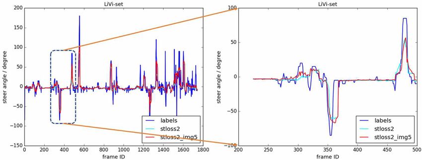
4      Peng Wan, Zhenbo Song, and Jianfeng Lu

of ALVINN demonstrates the potential of neural networks in autonomous driv-
ing. With the improvement of computing power and the development of deep
learning, many researchers use convolutional neural network(CNN) to achieve
environmental awareness and steering angle prediction. Nvidia [18] first used
the CNN to construct an autonomous driving system for robot in the DAVE
project. This system can control the vehicles to avoid obstacles safely. After
that, Nvidia built a PilotNet [1] network on autonomous vehicles to predict the
steering angle. This model performs well on simple highway roads with fewer
obstacles. Yang [19] analyzed the influence of features on the performance of
the end-to-end steering angle control model through experiments. The research
demonstrates that road-related features are indispensable, and roadside-related
features can improve the generalization of the model, but sky features do not
contribute to steering angle prediction. However, one disadvantage of the above
end-to-end work is that it only receives a single image as input, so it ignores
the temporal relationship between image frames. Considering the temporal re-
lationship between the image frames, Xu [2] and Chen [3] added LSTM to the
network to improve the prediction accuracy of the steering angle. In this work,
we use PilotNet as the feature extraction network. And in the same way, we
add LSTM to the end-to-end steering angle control network, which is composed
of CNN and LSTM. After receiving several continuous images as input, CNN
network extracts the features of visual input, and feeds the extracted sequence
features to LSTM for steering angle prediction.
    Fernandez [6] proposed a beam curvature method(BCM) method for obsta-
cle avoidance of mobile robots in unknown environments. The BCM method
combines beam method (BM) and curvature velocity method (CVM). In their
work [6], the beam method first calculate the best one-step heading then pass
it to CVM to calculate the optimal linear and angular velocities. In the local
navigation of the mobile robot, the system obtains the divergent radial projec-
tion model of the environment through the beam method. Then the BM method
calculates the best beam in the divergent radial projection model by applying
the objective function, and then obtains the current best local heading. After
that, Lopez [7] proposed a new local navigation approach for autonomous driving
vehicles, which combined the Pure pursuit method and BCM. Therefore, in our
autonomous vehicle system, end-to-end steering angle control model can also be
considered as a local navigation system. In our work, we adopt the similar idea
of BCM, which determines the best local navigation direction by building BM
model. We first calculate the horizontal angle and vertical angle corresponding
to each pixel, which are similar to the sector or radial beam in beam method,
and then input them into the network. Then the network combines the visual
input and the input of pixel-wise horizontal angle and vertical angle to predict
the current local steering angle.

2.2   Imbalanced Training
For the end-to-end steering angle prediction model, imbalanced training is a
great challenge at present. Since the car drives straight for most of the time,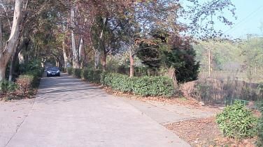
End-to-end Driving Model          5

therefore, most of the steering angle is close to 0 in real driving data. As for
imbalanced training, there are three ways to deal with this problem. One of
the methods is to amplify the dataset, namely, increase the number of samples
with the large steering angle. The main methods for dataset amplification are
to recollect data or use data enhancement methods. Although amplifying the
dataset is indeed an effective method, its cost is relatively high. In addition to
amplify the dataset, Qing [20] solves the problem of imbalanced training by re-
sampling the dataset. In their work, they divided the steering angle into 199
bins, then randomly selected some samples from each bin and kept the number
of samples in each box to no more than 2000. But this method may lose some
sample data, especially when the dataset is small, some important scene data
may be lost. The last method is to modify the loss function and apply different
weights to different losses to enhance the influence of small sample data. As
shown in the work of Wang [21] and Yang [22], they apply different loss weight
for different steering angle, the steering angle close to 0 is set a smaller weight
while the larger steering angle is set a larger weight. But they did not give
a specific loss function, it is difficult to determine the weights corresponding to
different steering angle errors. In other words, it is difficult to distinguish between
different steering angle errors. Aiming at this problem, Yuan [10] proposed a
novel cost-sensitive loss function, which was inspired by Lin’s idea [23]. They
analyzed the data distribution of steering angle, and considered that the steering
angle distribution was similar to the double long-tailed distribution. Finally,
the SteeringLoss based on this distribution was proposed. The loss function
can increase the influence of large steering angle while decrease the influence of
small steering angle. With SteeringLoss, the model can estimate a wider range of
steering angles. As SteeringLoss chooses mean square error (MSE) as the basic
function, MSE is more sensitive to outliers and it is difficult to predict small
steering angles. Therefore, we proposed our loss function and chose smoothL1 as
the basic function. With our loss function, the model can estimate the steering
angle more accurately, and the predicted steering angle range is wider than
SteeringLoss.

2.3   Driving Datasets
In order to train the end-to-end steering angle control model, some researchers
have collected some real-life driving datasets, such as LiVi-Set [3], BDD 100K
Dataset [24], Udacity Dataset. LiVi-Set contains video, point clouds and corre-
sponding steering angle and speed values. However, camera calibration data is
not included in the data, which is used to calculate the horizontal angle and
vertical angle. The main driving scenarios included in the dataset are urban
roads and highways. The BDD dataset contains only video, GPS and IMU, and
corresponding steering angle values is not collected. The steering angle values
is calculated by IMU information, so the accuracy of steering angle can not
be verified. Udacity Dataset mainly contains the image of the highway and the
corresponding steering angle data, but does not contain the image calibration
data. Our dataset contains images, camera calibration data, point clouds and
6       Peng Wan, Zhenbo Song, and Jianfeng Lu

corresponding throttle position, steering angle and brake position, and includes
multiple driving scenarios, such as urban, country, and off-road. The off-road
driving scene is not available in many datasets.

3     Methods

3.1   End-to-end Driving Model Combined with Pixel-wise
      Orientations

From previous work, it can be concluded that the end-to-end steering angle
prediction model is difficult to generate the accurate steering angle only based
on one single image. In the real driving scene, the driver’s driving behavior
is continuous. Therefore, similar to human driving behavior, many end-to-end
steering angle control models use continuous frames as input. On the one hand,
the CNN model can only extract the spatial features of a single image, so it
will ignore the temporal relationship between frames; on the other hand, as a
special form of RNN, LSTM can extract the temporal information of sequence
data. Therefore, we propose our end-to-end steering angle control model, which
combines the CNN network and the LSTM time series network. The overall
network architecture is shown in Fig. 1. In addition, considering that the size
of our training data is small, we use the light-weighted Pilotnet as the spatial
feature extraction layer for the image sequence. The PilotNet architecture is
shown in Fig. 2. In this work, we use the first 6 layers of PilotNet to encode visual
features, which includes 5 convolutional layers and 1 fully connected layer. The
first normalization layer normalizes the image and speeds up the convergence of
the network. The convolutional kernel size of the first three convolutional layers
is 5×5 and the stride size is 2×2, while the last two convolutional layers adopt a
3 × 3 kernel and a 1 × 1 stride. Then a fully connected layers of sizes 1024 follows
the convolutional layers. After PilotNet extracts the visual features, the encoded
features are forward to the LSTM layer. As seen in the whole pipline of the entire
network, the driving model takes the image sequence as input and encodes the
visual input through the PilotNet, where the image sequence includes the RGB
image and the pixel-wise horizontal angle map(HA Map) and vertical angles
map(VA Map). Then the encoded visual features are fed into the LSTM layer
to encode the temporal information. Finally, the network predicts the steering
angle according to the features encoded from LSTM.

3.2   Pixel-wise Orientations

As we mentioned above, our end-to-end steering angle control model can be sim-
ply regarded as local navigation. Most end-to-end control models use images as
visual input, which helps the end-to-end network to understand the surround-
ing scene and then realize the mapping from pixels to steering angles. But in
our work, we first calculate the pixel-wise orientations, which include the cor-
responding horizontal angle map and vertical angle map for each pixel in the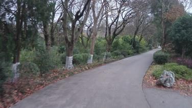
End-to-end Driving Model                  7

 Input planes
n@66×200 n@66×200                                                                       1024

                    24@31×98
                                                                              Flatten
                               36@14×47
                                           48@5×22     64@3×20       64@1×18

                           Normalization              Convolution[5×5]

                           Convolution[3×3]           Fully connected layer

Fig. 2: The PilotNet architecture. The PilotNet is used as a feature-
extracting sub-network to generate image features and forward the extracted
features to LSTM. n represents the channel of the input image.

image, and then concatenate the horizontal angle map and vertical angle map
with the image into a five-channel image. Finally, the synthesized image is fed
into the end-to-end driving model as input. By adding the pixel-wise orienta-
tions, the end-to-end steering angle control network can better understand the
heading angle of objects (such as cars, pedestrians, lane lines, etc.) relative to
the autonomous vehicle. With the relevant heading angle information, the end-
to-end network can avoid predicting the angle with obstacles as much as possible
when predicting the steering angle.
    Our driving scene can be simplified as shown in Fig. 3. As shown in Fig.
3, the scene under the field of view of the image is described by a frustum,
which is in the camera coordinate system. In order to describe the driving scene
conveniently in the image, we simplify the scene, which contains only one ball
used to represent objects. In this simplified scene, we assume that there is a point
P on the ball, and its imaging point in the image is P 0 . Afterwards, we project
the simplified scene along the positive direction of the y-axis and the negative
direction of the x-axis to obtain two projections in Fig. 4. As shown in Fig. 4, θ
and β are the horizontal angle and vertical angle of point P respectively. In Fig. 4,
the collision area indicated by the gray area. If the autonomous vehicle travels in
the gray area, it may collide with the object. Therefore, for the local navigation of
autonomous vehicles, the recognition of gray areas can help autonomous vehicles
avoid obstacles. If the horizontal angles and vertical angles corresponding to the
entire image are fed into the end-to-end steering angle control model, the model
can identify the corresponding gray area through learning, and then predict the
steering angle more accurately.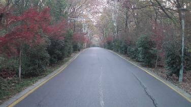
8      Peng Wan, Zhenbo Song, and Jianfeng Lu

                                                        P(x,y,z)

                                       P`(u,v)
                               z
                                                                   P`(u,v)
                               x
                          y                                 Image

Fig. 3: Local navigation scene. Our end-to-end driving model can be treated
as local navigation. The local navigation scene is simplified as a frustum under
the field of view angle of the image, which is in the camera coordinate system.
For convenience of expression, we use a ball to represent obstacles in the scene.
There is a point P on the ball, which is in the camera coordinate system, and
its imaging point P 0 in the image coordinate system.

   After simplifying the scene, we need to calculate the horizontal angle and
vertical angle of point P in Fig. 4, which are also the pixel-wise orientation of
point P 0 . According to the camera imaging principle, the relationship between
the point P and the pixel point P 0 can be expressed by the following formula:
                                             x
                                   u = fx ×    + cx                            (1)
                                             z
                                             y
                                    v = fy × + cy                              (2)
                                             z
    where cx , cy , fx , and fy are camera internal parameters. After that, we can
get the following formulation from Fig. 4:
                                           x
                                      tanθ =                               (3)
                                            z
                                            y
                                   tanβ =                                  (4)
                                            z
Combining the above four equations, we can calculate the horizontal angle and
vertical angle corresponding to each pixel by the following formulation:

                              θ = atan2(u − cx , fx )                          (5)

                              β = atan2(v − cy , fy )                          (6)

3.3   Loss Function
Since the existing relevant datasets are imbalanced, it is a challenge to train the
end-to-end steering angle control model. Before introducing the loss function,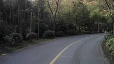
End-to-end Driving Model                             9

                              z

                                         P(x,y,z)
                                                                                              P(x,y,z)
                                                                                                               β
                                     θ                                                                                       z

                                                                                                               Ground Plane

                                                               y
                                                    x

Fig. 4: Projection of local navigation scene. The image on the left is pro-
jected along the positive direction of the y-axis, and the image on the right is
projected along the negative direction of the x-axis.

we first analyze the distribution of the imbalanced dataset, include LiVi-Set and
our dataset. The distribution of these two datasets is shown in Fig. 5. From
Fig. 5, we can see that there are some similarities in the distribution of steering
angle between the two datasets, their data distribution is similar to the long
tail distribution. In both datasets, most steering angle values are concentrated
near zero, and the larger the steering angle, the smaller the number of samples.
If the imbalanced dataset is used to train the end-to-end steering angle control
network, the network will tend to predict the smaller steering angle due to the
influence of large sample steering angles, which are close to 0.

                The steering angle distribution of LiVi-Set                         The steering angle distribution of PandoraDriving
         2500
                                                                            5000
         2000
                                                                            4000
Number

                                                                   Number

         1500
                                                                            3000
         1000                                                               2000

          500                                                               1000

            0                                                                  0
                150   100    50     0      50     100    150                       100   75     50   25    0     25    50    75    100
                       Steering value / degree                                                 Steering value / degree

Fig. 5: The steering value Distribution. This figure demonstrates the steer-
ing value distribution of LiVi-Set and PandoraDriving. The steering angle of left
turn relative to standard angle is less than 0, and that of right turn relative to
standard angle is greater than 0.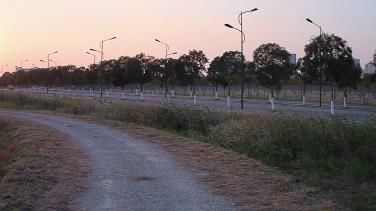
10      Peng Wan, Zhenbo Song, and Jianfeng Lu

    In order to solve the imbalanced training problem, we adopt the same basic
principles as [10, 21, 22]. The basic principle is that small steering angles are
assigned small weights, and large steering angles are assigned large weights. In
this way, the model can focus more on large steering angles. Therefore, Yuan’s
[10] proposed a cost-sensitive loss function, which called SteeringLoss. By using
SteeringLoss as the loss function, the end-to-end model can estimate a wider
range of steering angles. In our work, we use modified the SteeringLoss and
propose our loss function, which is called SteeringLoss2. The SteeringLoss is
defined as follows:
                                     n
                                 1 X
                       loss =          (1 + α|yi |γ )δ (yi − yi0 )2              (7)
                                2n i=1

where n is the total number of samples, yi is the ground truth of ith sample, and
yi0 is estimation value of ith sample, α, γ, δ are hyperparameters. SteeringLoss is
based on mean square error (MSE), which is sensitive to outlier. Besides, when
there is a big difference between the estimated value and ground truth, MSE
is easy to cause gradient explosion. In the end-to-end steering angle control
model, the MSE based model is difficult to estimate the small steering angle
accurately because the MSE is more sensitive to the large steering angle. In the
MSE based SteeringLoss, although the SteeringLoss can pay more attention to
the large steering angle by assigning a large weight to the large steering angle,
it is difficult to predict the small steering angle due to the influence of the basic
function MSE. Therefore, we modify SteeringLoss and design our loss function
as follows:
                                n
                             1X
                     loss =        (1 + α|yi |γ )smoothL1 (|yi − yi0 |)           (8)
                             n i=1

in which                              (
                                          0.5x2 , |x| ≤ 1
                    smoothL1 (x) =                                               (9)
                                          |x| − 0.5, otherwise

where n is the total number of samples, yi is the ground truth of ith sample,
and yi0 is estimation value of ith sample. In the SteeringLoss2, we discard the
hyperparameter δ, because by setting the hyperparameter γ, the same effect as
the hyperparameter δ can be achieved. The Steeringloss2 is a cost-sensitive loss
function based on smoothL1 , while SteeringLoss is based on MSE. The reason
why we choose smoothL1 as the basic function is that smoothL1 not only has
the robustness of mean absolute error (MAE) but also can solve the gradient
explosion problem of MSE. In the back propagation of neural network, since the
update gradient of MAE remains unchanged, the model is difficult to converge
when the loss is small. When the difference between the estimation value and
the ground truth is small, smoothL1 uses MSE, which can solve the problem of
constant update gradient of MAE. When the difference between the estimation
value and the ground truth is large, the MAE is used in smoothL1 . Although the
end-to-end steering angle control model based on smoothL1 predicts the small
End-to-end Driving Model 11
steering angle, the model based on SteeringLoss2 pays more attention to the large
steering angle by assigning large weights to large steering angles. Therefore, the
model based on SteeringLoss2 can predict both small steering angle and large
steering angle.
4 Experimental
4.1 Dataset Description
In our work, LiVi-Set Prepared Dataset and our own collected datasets are
used to verify our proposed method. The LiVi-Set contains point clouds, video,
and corresponding driving behavior data, where the video is captured by the
minor distortion dashboard camera. This raw dataset they provided has not been
preprocessed and there are some video and driving behavior data misalignments,
which will lead to poor performance of the model. In order to reduce the impact
of noise on the performance of the model, we use their prepared dataset with
few errors, although the prepared dataset size is small. In addition, the image
resolution in the LiVi-Set is 1920 × 1080, while the input image resolution of our
model is 200 × 66, so we need to preprocess the original data. We first cropped
the image area related to the sky and the hood of the autonomous car, and then
scaled it to the size of 200 × 66.
The driving scenarios in the LiVi-Set prepared dataset are mostly urban roads
and highways. In order to verify whether our method is suitable for a variety of
driving scenarios, we collected our own dataset through our own experimental
platform and named it Pandoradriving. The experimental platform is equipped
with Pandora lidar camera sensing kit made in China, which can simultaneously
collect point clouds of 40 lines laser around the platform, color high-definition
images in front of the vehicle, panoramic black-and-white images. Basides visual
information, we also collect the driving behaviors through the Controller Area
Network (CAN) bus. The collected driving behaviors include throttle position,
steering angle, and brake position. In order to align the driving behavior data
with the visual input, we adopt the network time alignment on the experimental
platform, in which Pandora and CAN bus work at 10HZ.
Our dataset contains 18 different color image sequences, point clouds se-
quences, and corresponding behavior data. The total collection time is more
than 40 minutes, and the total number of images collected is more than 25000
frames. Our dataset includes multiple driving scenarios,such as urban, country
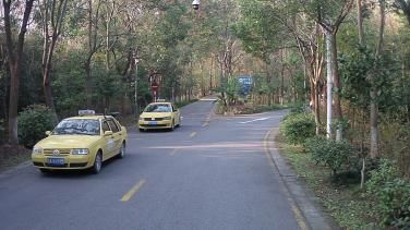
and off-road. As shown in Fig. 6, we extracted some representative data from
PandoraDriving, including corresponding images, point clouds, and steering an-
gles in different scenes.
The main goal of our work is to train the end-to-end steering angle control
model, so we only use images and corresponding driving behavior data. Since
the network for image is 200 × 66, and the image resolution in our dataset is
1280 × 720, the image needs to be cropped and scaled before feeding into the
network. We use the same processing method as LiVi-Set, first cropped the image12 Peng Wan, Zhenbo Song, and Jianfeng Lu
-24.0 degree -5.9 degree 1.2 degree 4.9 degree 18.4 degree 44.3 degree
Fig. 6: The representative examples in PandoraDriving. Examples include
RGB images, point clouds, and corresponding steering angles in multiple driving
scenarios, where driving scenarios include cities, rural areas, and suburbs. First
row is the RGB image, second row is the corresponding point clouds and the
last row is the corresponding steering angle.
area of the car hood and the sky, and then scaled it to the specified size. When
the steering wheel turns left relative to the standard angle, the steering wheel
value is less than 0. Similarly, the steering wheel greater than 0 indicates that
the steering wheel turns right relative to the standard angle. In addition, the
range of the steering angle collected in the dataset is [−π × 1000, π × 1000], and
the corresponding real steering angle is [−π, π], so we need to scale all the raw
steering angles to [−π, π].
4.2 Evaluation Metric
In order to evaluate the performance of the end-to-end steering angle prediction
model, the researchers proposed different evaluation metric. In PilotNet, they
used the calculation of the number of manual interventions as evaluation metric
in the simulation test, while in the on-road test, the proportion of autonomous
driving time was used as evaluation metric. However, the evaluation metric can-
not distinguish the different levels of bad predictions. In other words, we cannot
distinguish the difference between the estimated steering angle and the ground
truth by 5 degrees and 15 degrees. Xu [2] proposed a driving perplexity as an
evaluation criterion, which is inspired by language modeling metric. However,
this evaluation metric does not give meaning to the real world, nor can it judge
whether the model is effective. In other words, it is difficult to judge the specific
difference between the predicted value and the real value from the evaluation
metric. Accuracy metric is widely adopted in [3, 18, 25], and the accuracy metric
is more intuitive than the driving perplexity. Therefore, we also adopt the accu-
racy metric in our work. In order to facilitate the calculation accuracy, we need to
use the tolerance threshold. We believe that in the real world, the driver’s driv-
ing behavior also has a small deviation, so it is reasonable to use the tolerance
threshold. In our work, We chose 5◦ as the steering angle tolerance threshold,End-to-end Driving Model 13 while Chen [3] choose 6◦ as the the steering angle tolerance threshold. In ad- dition to using accuracy as the evaluation criterion, we also use the standard deviation (SD) of the estimated value to evaluate the model, which is also used in [10]. SD is used to evaluate the value range of the steering angle estimated by the model. The larger the SD of the estimated steering angle, the wider the steering angle can be predicted by the model. In other words, if the SD of the steering angle estimated by the model is larger, it indicates that the model can estimate the larger steering angle instead of only estimating the steering angle close to 0. 4.3 Results In order to verify the impact of the SteeringLoss2 on the performance of the model, we did four comparative experiments using MAE, MSE, SteeringLoss and SteeringLoss2 as the loss function. All experiments are based on the model shown in Fig. 1. At this time, the input of the model is the RGB image sequence, and the structure of the network feature extraction module is shown in Fig. 2. The steering angle prediction accuracy of our experiments is shown in Table 1, where the steering angle tolerance threshold is set to 5 degrees, and the parame- ter α, γ and δ are set to 1.0. To further investigate the performance of the model under different loss functions, Fig. 7 plots the ground truth of consecutive frames collected from human and the corresponding predicted steering angle values. In addition, in order to observe the difference between the predicted value and the ground truth in more detail, some consecutive frames are selected from the left sub-figure for display, and the results are shown on the right sub-figure in Fig. 7. As shown in Table 1, the model using SteeringLoss2 as the loss function has the highest prediction accuracy, while the model using MSE as the loss function has the lowest prediction accuracy. MSE calculates the square of the distance between the ground truth and the estimation, while MAE only calculates the absolute error between the ground truth and the estimation. In other words, MSE is more sensitive to outliers than MAE. Therefore, in imbalanced training, due to the higher proportion of steering angles close to 0 degrees, the steering angles predicted by MAE are relatively close to 0, and it is difficult to predict large steering angles. As can be seen from the prediction results of LiVi-set in Fig. 7, the steering angle predicted by MAE between 340 and 380 frames is closer to zero than other loss functions. On the contrary, the model using MSE as the loss function is vulnerable to the influence of large steering angle, which makes the predicted steering angle very unstable, and the prediction accuracy of small steering angle with high proportion is worse than MAE. Therefore, the prediction accuracy of the model with MAE loss function is higher than that of MSE loss function which is sensitive to large steering angle. It can be seen from Table 1 that the prediction accuracy of the model using the SteeringLoss or SteeringLoss2 is higher, which also proves that the cost-sensitive loss function is effective in the imbalanced training. Compared with the traditional loss function, this cost-sensitive loss function can improve the model’s attention to large steer- ing angle by applying larger weight to large steering angle and smaller weight to
14     Peng Wan, Zhenbo Song, and Jianfeng Lu

small steering angle, so as to maintain the prediction accuracy of small steering
angle and improve the prediction of large steering angle. Observing the impact of
the two cost-sensitive loss functions on the performance of the model, it can be
seen that the prediction accuracy of the improved loss function SteeringLoss2 is
better than that of the SteeringLoss. Furthermore, the proposed SteeringLoss2
choose smoothL1 as the basic function, which has the robustness of MAE, and
at the same time will not be too sensitive to outliers like MSE. Therefore, the
prediction accuracy of SteeingLoss is higher than MSE, while SteeringLoss2 per-
forms best. In addition to the observation accuracy, it can be observed from SD
that the SD of the steering angle predicted by the model using MAE as the
loss function is the smallest. The reason is that MAE is affected by the small
steering angle, which accounts for a high proportion of the number of samples,
and its predicted steering angle is small, so it cannot cope with the scene of
large steering angle, which leads to the smallest SD value. On the contrary, the
model with cost-sensitive loss function can get larger SD than the traditional
loss function. In addition, it can be found that the model with SteeringLoss as
the loss function on the LiVi-set has a larger SD value, but combining with Fig.
7, it can be seen that most of the steering angles predicted by SteeringLoss are
larger than the ground truth, so the SD value is large and the accuracy is low.
When SteeringLoss2 is used as the loss function on PandoraDriving, the model
gets the largest SD, which also confirms that the cost-sensitive loss function
SteeringLoss2 can predict a relatively large steering angle, and the predicted
steering angle is also more accurate.

Table 1: Performance of models with different loss functions. Accuracy
represents the prediction accuracy of the steering angle of the model. SD rep-
resents the standard deviation of the steering estimation value. The accuracy is
measured within 5◦ biases.
                                 LiVi-Set               PandoraDriving
       loss function
                           Accuracy          SD       Accuracy       SD
           MAE              66.3%           5.34       72.2%         9.58
           MSE              56.3%           12.97      69.4%        15.34
       SteeringLoss         61.8%           16.37      69.7%        15.57
       SteeringLoss2        67.0%           14.73      76.4%        22.99

    In order to verify the influence of pixel-wise orientations on network per-
formance, we concatenate the pixel-wise orientations with RGB image matrix
into five-channel input matrix. In addition, it can be seen from Table 1 that
the accuracy and SD of the cost-sensitive loss function used by the network are
better than the traditional loss function. Therefore, the comparison experiment
here uses cost-sensitive loss functions, and compares the effect of pixel-wise ori-
entations on the performance of the model through experiments. The model
performance are shown in Table 2, and the comparison performance between
the visualized predicted steering angle and the ground truth are shown in Fig.
End-to-end Driving Model 15
8. As shown in Table 2, after adding the pixel-wise orientations as an additional
input, the accuracy of the network and the SD of the predicted steering angle are
higher than those of the network using only RGB images as input. In addition, it
can be seen from Fig. 8 that the steering angle predicted by the network is closer
to the ground truth after adding the pixel-wise orientations. This proves that
the network can recognize the object in the image and predict more accurate
steering angle information through the learning of direction-aware features. At
the same time, the standard deviation of the predicted steering angle is slightly
larger, which indicates that the model can predict large steering angle.
(a) LiVi-Set
(b) PandoraDriving Dataset
Fig. 7: Comparison of the ground truth and the predicted steering of the network
under different loss functions. In the figure, stloss is the model with SteeringLoss,
stloss2 is the model with SteeringLoss2, and label is the ground truth. The right
sub-figure is the sub-sequence of the left sub-figure such that more detailed
difference can be clearly observed.
There is a mapping relationship between the pixel-wise orientations and the
pixels in the RGB image. In other words, each pixel has its corresponding hor-
izontal angle information and vertical angle information. Therefore, we believe
that the orientations also has a mapping relationship with the image feature16 Peng Wan, Zhenbo Song, and Jianfeng Lu
Table 2: Performance of models with different input. Accuracy represents
the prediction accuracy of the steering angle of the model. SD represents the
standard deviation of the steering estimation value. The accuracy is measured
within 5◦ biases.
LiVi-Set PandoraDriving
Input + loss function
Accuracy SD Accuracy SD
RGB + SteeringLoss2 67.0% 14.73 76.4% 22.99
RGB + pixel-wise orientations + SteeringLoss2 67.9% 15.12 77.9% 25.52
maps extracted by the convolutional layer, because the feature maps extracted
by the CNN network is obtained by the image through the convolution operation.
We scale the pixel-wise orientations to the size of the corresponding convolution
feature maps and splice them into fusion features. To further verify the influence
of the fusion feature on the network performance, we have done some compar-
ison experiments. The experimental results are shown in Table 3. We denote
the output features of the first five convolutional layers as {conv1, conv2, conv3,
conv4, conv5}. For output feature map from each convolutional layer, we need to
calculate its corresponding orientations, which is obtained by scaling the pixel-
wise orientations corresponding to the original RGB. The obtained orientations
is concatenated with the output feature maps, and then the fusion features are
further forwarded to the next layer. As shown in Table 3, the prediction accuracy
of the network is the highest after the orientations is concatenated with the out-
put feature map of the third convolution layer, but its corresponding standard
deviation is the lowest, which indicates that the range of steering angle predicted
by this model is slightly smaller. Although the prediction accuracy of the model
is not the highest after the orientations and RGB images are concatenated, the
standard deviation of the steering angle predicted by the model is higher in
all the comparision experiments. Considering the results in Table 3, we choose
to concatenate the orientations with RGB image, because this model can not
only maintain high prediction accuracy, but also has high standard deviation of
predicted value.
Table 3: Performance of models after concatenate the pixel-wise ori-
entations with the output of different convolutional layers. All models
use SteeringLoss2 as loss function. The accuracy is measured within 5◦ biases.
LiVi-Set PandoraDriving
Accuracy SD Accuracy SD
RGB + VA Map + HA Map 67.9% 15.12 77.9% 25.52
conv1 + VA Map + HA Map 68.0% 15.07 75.5% 23.67
conv2 + VA Map + HA Map 68.0% 14.90 72.3% 26.20
conv3 + VA Map + HA Map 68.6% 14.75 78.1% 21.92
conv4 + VA Map + HA Map 68.4% 15.10 77.2% 22.73
conv5 + VA Map + HA Map 68.5% 14.91 75.5% 22.14End-to-end Driving Model 17
(a) LiVi-Set
(b) PandoraDriving Dataset
Fig. 8: Comparison of the ground truth and the predicted steering of the network
under different inputs. In the figure, stloss is the model with SteeringLoss, stloss2
is the model with SteeringLoss2, and label is the ground truth. The right sub-
figure is the sub-sequence of the left sub-figure such that more detailed difference
can be clearly observed.
5 Conclusions and Future Work
In this paper, we propose a novel end-to-end steering angle control model, which
takes RGB images and their corresponding pixel-wise orientations as input. In
the whole process of generating the corresponding steering angle, our driving
scene can be treated as the local navigation of the autonomous car, so we adopt
the idea similar to the BM algorithm of robot local navigation, and propose the
pixel-wise orientations of the RGB images. Then we concatenate the pixel-wise
orientations with the RGB image as the network input, the orientations are sim-
ilar to the sector or radial in the BM model. After adding the pixel-wise orienta-
tions, the end-to-end steering angle control model can predict the steering angle
more accurately than only receiving RGB images as input. After that, In order
to deal with the problem of steering angle imbalance, we propose SteeringLoss2,18 Peng Wan, Zhenbo Song, and Jianfeng Lu
which is an improved version of SteeringLoss. Through experiments, we found
that SteeringLoss2 has the best performance, which can not only maintain the
robustness of MAE, but also avoid further amplification error of SteeringLoss,
and the model based on SteeringLoss2 can estimate a wider range of steering
angles. Besides, we also present our own datasets, which includes multiple driv-
ing scenarios. Finally, we conduct some comparison experiment on LiVi-Set and
our own dataset, and the experiment shows that the model using our proposed
methods can predict steering angle accurately.
Although our method can estimate a wider steering angle, there is still a
large deviation between the estimated steering angle and the ground truth, which
leads to insufficient prediction accuracy. In future work, we will feed the point
clouds into the end-to-end steering angle control model. Different from two-
dimensional images, the point clouds has rich depth information and geometric
features, which can help the control model make better decisions.
References
1. Mariusz Bojarski, Davide Del Testa, Daniel Dworakowski, et al. End to end learn-
ing for self-driving cars. arXiv: Computer Vision and Pattern Recognition, 2016.
2. Huazhe Xu, Yang Gao, Fisher Yu, and Trevor Darrell. End-to-end learning of driv-
ing models from large-scale video datasets. In Proceedings of the IEEE conference
on computer vision and pattern recognition, pages 2174–2182, 2017.
3. Yiping Chen, Jingkang Wang, Jonathan Li, Cewu Lu, Zhipeng Luo, Han Xue, and
Cheng Wang. Lidar-video driving dataset: Learning driving policies effectively. In
Proceedings of the IEEE Conference on Computer Vision and Pattern Recognition,
pages 5870–5878, 2018.
4. Sepp Hochreiter and Jürgen Schmidhuber. Long short-term memory. Neural com-
putation, 9(8):1735–1780, 1997.
5. Tharindu Fernando, Simon Denman, Sridha Sridharan, and Clinton Fookes. Going
deeper: Autonomous steering with neural memory networks. In Proceedings of the
IEEE International Conference on Computer Vision Workshops, pages 214–221,
2017.
6. Joaquı́n Lopez Fernández, Rafael Sanz, JA Benayas, and Amador R Diéguez. Im-
proving collision avoidance for mobile robots in partially known environments: the
beam curvature method. Robotics and Autonomous Systems, 46(4):205–219, 2004.
7. J López, C Otero, R Sanz, E Paz, E Molinos, and R Barea. A new approach to
local navigation for autonomous driving vehicles based on the curvature velocity
method. In 2019 International Conference on Robotics and Automation (ICRA),
pages 1751–1757. IEEE, 2019.
8. Prahlad Vadakkepat, Kay Chen Tan, and Wang Ming-Liang. Evolutionary arti-
ficial potential fields and their application in real time robot path planning. In
Proceedings of the 2000 congress on evolutionary computation. CEC00 (Cat. No.
00TH8512), volume 1, pages 256–263. IEEE, 2000.
9. Jia Deng, Wei Dong, Richard Socher, Li-Jia Li, Kai Li, and Li Fei-Fei. Imagenet:
A large-scale hierarchical image database. In 2009 IEEE conference on computer
vision and pattern recognition, pages 248–255. IEEE, 2009.
10. Wei Yuan, Ming Yang, Hao Li, Chunxiang Wang, and Bing Wang. Steeringloss: A
cost-sensitive loss function for the end-to-end steering estimation. IEEE Transac-
tions on Intelligent Transportation Systems, 2020.End-to-end Driving Model 19
11. Chenyi Chen, Ari Seff, Alain Kornhauser, and Jianxiong Xiao. Deepdriving: Learn-
ing affordance for direct perception in autonomous driving. In Proceedings of the
IEEE International Conference on Computer Vision, pages 2722–2730, 2015.
12. Alexandru Gurghian, Tejaswi Koduri, Smita V Bailur, Kyle J Carey, and Vidya N
Murali. Deeplanes: End-to-end lane position estimation using deep neural net-
worksa. In Proceedings of the IEEE Conference on Computer Vision and Pattern
Recognition Workshops, pages 38–45, 2016.
13. Mariusz Bojarski, Anna Choromanska, Krzysztof Choromanski, Bernhard Firner,
Larry J Ackel, Urs Muller, Phil Yeres, and Karol Zieba. Visualbackprop: Effi-
cient visualization of cnns for autonomous driving. In 2018 IEEE International
Conference on Robotics and Automation (ICRA), pages 1–8. IEEE, 2018.
14. Jinkyu Kim and John Canny. Interpretable learning for self-driving cars by visu-
alizing causal attention. In Proceedings of the IEEE international conference on
computer vision, pages 2942–2950, 2017.
15. Mariusz Bojarski, Philip Yeres, Anna Choromanska, Krzysztof Choromanski, Bern-
hard Firner, Lawrence Jackel, and Urs Muller. Explaining how a deep neural net-
work trained with end-to-end learning steers a car. arXiv: Computer Vision and
Pattern Recognition, 2017.
16. Lu Chi and Yadong Mu. Learning end-to-end autonomous steering model from spa-
tial and temporal visual cues. In Proceedings of the Workshop on Visual Analysis
in Smart and Connected Communities, pages 9–16, 2017.
17. Dean A Pomerleau. Alvinn: An autonomous land vehicle in a neural network. In
Advances in neural information processing systems, pages 305–313, 1989.
18. Urs Muller, Jan Ben, Eric Cosatto, Beat Flepp, and Yann L Cun. Off-road ob-
stacle avoidance through end-to-end learning. In Advances in neural information
processing systems, pages 739–746, 2006.
19. Shun Yang, Wenshuo Wang, Chang Liu, Weiwen Deng, and J Karl Hedrick. Feature
analysis and selection for training an end-to-end autonomous vehicle controller
using deep learning approach. In 2017 IEEE Intelligent Vehicles Symposium (IV),
pages 1033–1038. IEEE, 2017.
20. Qing Wang, Long Chen, Bin Tian, Wei Tian, Lingxi Li, and Dongpu Cao. End-to-
end autonomous driving: An angle branched network approach. IEEE Transactions
on Vehicular Technology, 68(12):11599–11610, 2019.
21. Dan Wang, Junjie Wen, Yuyong Wang, Xiangdong Huang, and Feng Pei. End-to-
end self-driving using deep neural networks with multi-auxiliary tasks. Automotive
Innovation, 2(2):127–136, 2019.
22. Zhengyuan Yang, Yixuan Zhang, Jerry Yu, Junjie Cai, and Jiebo Luo. End-to-end
multi-modal multi-task vehicle control for self-driving cars with visual perceptions.
In 2018 24th International Conference on Pattern Recognition (ICPR), pages 2289–
2294. IEEE, 2018.
23. Tsung-Yi Lin, Priya Goyal, Ross Girshick, Kaiming He, and Piotr Dollár. Focal
loss for dense object detection. In Proceedings of the IEEE international conference
on computer vision, pages 2980–2988, 2017.
24. Fisher Yu, Haofeng Chen, Xin Wang, et al. Bdd100k: A diverse driving dataset for
heterogeneous multitask learning. In Proceedings of the IEEE/CVF Conference on
Computer Vision and Pattern Recognition, pages 2636–2645, 2020.
25. Jiman Kim and Chanjong Park. End-to-end ego lane estimation based on sequen-
tial transfer learning for self-driving cars. In Proceedings of the IEEE Conference
on Computer Vision and Pattern Recognition Workshops, pages 30–38, 2017.You can also read