On spatial conditional extremes for ocean storm severity - Lancaster ...
←
→
Page content transcription
If your browser does not render page correctly, please read the page content below
Environmetrics 00, 1–29
DOI: 10.1002/env.XXXX

On spatial conditional extremes for ocean
storm severity

R. Shootera∗ , E. Rossb , J. Tawnc and P. Jonathanc,d

Summary: We describe a model for the conditional dependence of a spatial process measured at one or more
remote locations given extreme values of the process at a conditioning location, motivated by the conditional
extremes methodology of Heffernan and Tawn. Compared to alternative descriptions in terms of max-stable
spatial processes, the model is advantageous since it is conceptually straightforward, and admits different
forms of extremal dependence (including asymptotic dependence and asymptotic independence). We use the
model within a Bayesian framework to estimate the extremal dependence of ocean storm severity (quantified
using significant wave height, HS ) for locations on spatial transects with approximate east-west (E-W) and
north-south (N-S) orientations in the northern North Sea (NNS) and central North Sea (CNS). For HS on
standard Laplace marginal scale, the conditional extremes “linear slope” parameter α decays approximately
exponentially with distance for all transects. Further, the decay of mean dependence with distance is found
to be faster in CNS than NNS. The persistence of mean dependence is greatest for the E-W transect in NNS,
potentially since this transect is approximately aligned with the direction of propagation of the most severe
storms in the region.

Keywords: conditional extremes, spatial dependence, non-stationary, significant wave height

  a
    STOR-i Centre for Doctoral Training, Department of Mathematics and Statistics, Lancaster University LA1 4YR, United
Kingdom.
b
  Shell Global Solutions International BV, Amsterdam, The Netherlands.
c
  Department of Mathematics and Statistics, Lancaster University LA1 4YW, United Kingdom.
d
  Shell Research Ltd., London SE1 7NA, United Kingdom.
∗
  Correspondence to: r.shooter@lancaster.ac.uk

     This paper has been submitted for consideration for publication in Environmetrics
Environmetrics                               R. Shooter, E. Ross, J. Tawn, and P. Jonathan

1. INTRODUCTION

Quantifying extreme ocean environments is important for safe and reliable construction and
operation of offshore and coastal infrastructure. Extreme value analysis provides a framework
within which the marginal and dependence characteristics of extreme ocean environments
can be estimated, and joint inferences corresponding to very long periods of observation
made in the presence of non-stationarity with respect to covariates.

The spatial structure of ocean surface roughness within a storm is of particular concern when
inferences are based on observations from multiple locations in a neighbourhood. For a given
ocean basin, when the distance between two locations is small relative to the spatial extent
of a storm low pressure field, it is reasonable to expect that large values of ocean surface
roughness (for a period of time of the order of an hour, quantified in terms of significant
wave height HS ) at the two locations will be dependent. Moreover, the extent of this spatial
dependence will potentially itself be non-stationary with respect to covariates, such as
storm direction and season. A reasonable statistical description of HS on a neighbourhood
of locations should therefore admit appropriately flexible descriptions of extremal spatial
dependence. Incorrect specification or estimation of the dependence structure can lead to
misleading joint predictions of HS on the neighbourhood. We note a number recent articles
on spatial extremes with at least some synoptic content, including Davison et al. (2012),
Reich and Shaby (2012), Ribatet (2013), Huser and Wadsworth ((2019 to appear) and Tawn
et al. (2018).

A number of recent studies explore the extremal spatial dependence of HS . For example,
Kereszturi et al. (2016) assesses the extremal dependence of North Sea storm severity
using the summary statistics χ and χ̄ (or equivalently η, Coles et al. 1999), outlined in
Section 3. Estimates for these summary statistics were used to categorise observed extremal
dependence as either asymptotic dependence (AD, suggesting that extreme events tend to

                                             2
On spatial conditional extremes for ocean storm severity                 Environmetrics

occur simultaneously) or asymptotic independence (AI, suggesting that extreme events are
unlikely to occur together); further discussion of these concepts is given in Section 3.1. In
Kereszturi et al. (2016), it was found that, in most cases considered, asymptotic independence
seemed to be the more appropriate assumption, compared to the assumption of asymptotic
dependence. Kereszturi (2016) and Ross et al. (2017a) extend this assessment to include the
estimation of a number of max-stable process (MSP) and inverted MSP models (Wadsworth
and Tawn, 2012), including the so-called Smith (Smith, 1990), Schlather (Schlather, 2002)
and Brown-Resnick (Brown and Resnick, 1977) models, and corresponding models for the
inverted processes. For all models considered there is evidence that the extremal dependence
of HS at two locations varies with the distance between the locations, and their relative
orientation.

By construction, MSP models considered in Kereszturi (2016) and Ross et al. (2017a) exhibit
AD exclusively, whereas inverted MSP models only exhibit AI. In general, we do not know
a priori which form of extremal dependence is more appropriate: a decision concerning the
form of extremal dependence present in the sample must therefore be made before parameter
estimation; this is less than ideal, although estimation of χ and χ̄ can aid this choice.
We note alternative AD models including those of Reich and Shaby (2012), Ferreira and
de Haan (2014), Rootzen et al. (2018), Kiriliouk et al. (2018 to appear). A number of more
sophisticated hybrid models have been proposed (e.g. Wadsworth and Tawn 2012, Wadsworth
et al. 2017, Huser and Wadsworth (2019 to appear) spanning dependence classes, but these
tend to be rather computationally challenging to estimate in practice.

The conditional extremes model of Heffernan and Tawn (2004) provides an alternative
approach to characterising extremal spatial dependence admitting both AI and AD. The
conditional extremes model also allows the incorporation of covariate effects (e.g. Jonathan
et al. 2014). In the current work, we propose an extension of the conditional extremes method
to a spatial setting, known as the spatial conditional extremes (SCE) model. SCE provides a

                                              3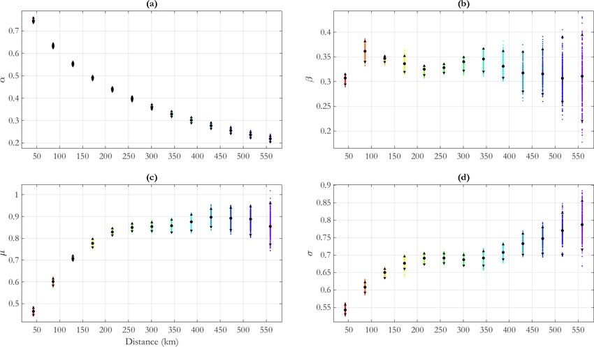
Environmetrics                               R. Shooter, E. Ross, J. Tawn, and P. Jonathan

framework to quantify the extreme marginal and dependence structure of HS for locations in
a neighbourhood, including the behaviour of extremal dependence of HS at different locations
as a function of the relative displacements of locations. Model estimation can be achieved
using a relatively straightforward Markov chain Monte Carlo (MCMC) scheme, and unlike
for MSP models, does not require composite likelihood techniques for parameter estimation
and hence does not incur parameter bias, as detailed in Tawn et al. (2018) and Wadsworth
and Tawn (2018).

The layout of the article is as follows. In Section 2, we present motivating applications
involving samples of HS on spatial neighbourhoods in the northern and central North Sea.
Section 3 outlines the spatial conditional extremes model. Parameter estimation is performed
using Bayesian inference as described in Section 4; details of parameter constraints from Keef
et al. (2013a), and the Metropolis-within-Gibbs sampling scheme, are given in the Appendix.
Results of the application of the SCE model to the north-south transect of the northern North
Sea sample are given in Section 5, with corresponding results for the east-west transect (for
the northern North Sea), and north-south and east-west transects for the central North Sea
reported in Section 6. Section 7 provides discussion and conclusions.

2. MOTIVATING APPLICATION

We consider hindcast data for storm peak significant wave height (henceforth HS for brevity)
from two neighbourhoods, one in the northern North Sea (NNS) and one in the central North
Sea (CNS), as illustrated in Figure 1. In each neighbourhood, values for HS are available on
north-south (N-S) and east-west (E-W) transects intersecting at a central location.

                                   [Figure 1 about here.]

The NNS sample corresponds to winter storms (occurring in winter months October-March)
                                              4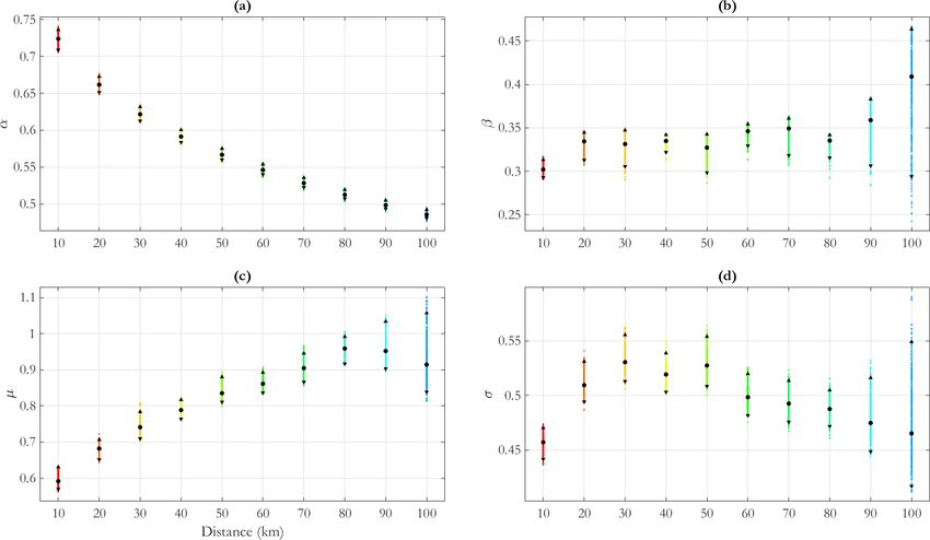
On spatial conditional extremes for ocean storm severity                Environmetrics

from the NEXTRA hindcast (Oceanweather 2002) for 20 locations on the two transects.
Storm intervals for a total of 1680 storms during the period 1 Oct 1964 to 31 Mar 1995
were isolated from up- and down-crossings of a sea state significant wave height threshold
for the central location, using the procedure outlined in Ewans and Jonathan (2008). Storm
peak significant wave height for each storm interval at each location provided a sample
of 1680 × 20 observations for further analysis. For each storm-location combination, the
direction (from which waves emanate, measured clockwise from North) at the time of the
storm peak, referred to as the storm direction, was also retained. The spatial extremal
characteristics of this sample have been examined previously in Ross et al. (2017a); further
discussion and illustrations of the data are available there.

The CNS sample corresponds to hindcast storm peak events (occurring at any time of year)
for a period of 37 years from 10 January 1979 to 30 December 2015 for 21 locations on
the two transects. The hindcast uses CFSR wind fields (Saha et al. 2014) and a MIKE21
spectral wave simulator model (Sorensen et al. 2005) to generate storm time-series at each
location. Storm periods were again identified as exceedances of a threshold non-stationary
with respect to season and direction, using the procedure of Ewans and Jonathan (2008) for
the central location. In this way, a total of 3104 storm events were isolated per location for
further analysis.

As will be explained further in Section 3, the SCE model is most conveniently considered
for data with marginal standard Laplace distributions. For simplicity, we therefore choose to
transform the NNS and CNS samples to standard Laplace scale prior to spatial conditional
extremes analysis, as suggested by Keef et al. (2013b), for example. This is achieved by
estimating non-stationary marginal models (directional for NNS and directional-seasonal for
CNS), following the approach of Ross et al. (2017a) and Ross et al. (2017b), independently
per location. Transformed data then follow a standard Laplace distribution for each location.

Figure 1 illustrates that the inter-location spacing for the NNS hindcast is considerably

                                               5
Environmetrics R. Shooter, E. Ross, J. Tawn, and P. Jonathan
larger than for the CNS hindcast. For this reason, it is important we compare the variation
of extremal spatial dependence between locations explicitly as a function of physical distance
(here in kilometres, km). Scatter plots of Laplace-scale storm peak HS for pairs of locations
separated by distances of 43.0, 171.8 and 300.7 km along the NNS north-south (NNS:N-S)
transect, coloured red in Figure 1, are shown by the black points in Figure 4 (see Section 5.1).
3. SPATIAL CONDITIONAL EXTREMES
3.1. Characterising extremal dependence
Key concepts in assessing extremal dependence are the notions of asymptotic dependence
(AD) and asymptotic independence (AI). Typically, these are assessed through calculating
two quantities, χ and χ̄ introduced by Coles et al. (1999). For bivariate data (X, Y ) with
common margins, the quantity χ is calculated as
χ = lim P(Y > u|X > u),
u→uF
where uF is the upper endpoint of the common marginal distribution F of the random
variables. Then χ̄ is defined by Coles et al. (1999) as χ̄ = 2η − 1. Here, η, known as the
coefficient of tail dependence, is defined by Ledford and Tawn (1996) from the asymptotic
approximation, as z → uF ,
1
P(X > z)1/η ,
P(X > z, Y > z) ∼ L
P(X > z)
where L(w) is a slowly varying function, so that L(tw)/L(w) → 1 as w → ∞ for t > 0. Coles
et al. (1999) provide details on how to calculate estimates for χ and χ̄. Then χ > 0 defines
the extent of AD present, whereas χ = 0 suggests the variables exhibit AI. In the latter
case, χ measures the extent of AI present. Tawn et al. (2018) present a spatial equivalent
6On spatial conditional extremes for ocean storm severity Environmetrics
for these measures. Crucially, the spatial characteristics under these two limiting extremal
behaviour types are very different; under AD, two (or more) extreme events may occur at
separate sites simultaneously, whilst under AI this is not the case. Realistically, a spatial field
is likely to exhibit a mixture of these behaviours: at short inter-location distance, asymptotic
dependence may prevail; for sites a large distance apart, asymptotic independence is more
likely, leading to independence at very large distances. The SCE model accommodates both
these possibilities.
3.2. The conditional extremes model of Heffernan and Tawn (2004)
In its simplest form, for a sample from a pair (X, Y ) of random variables with Laplace
marginal distributions, for x larger than some suitable threshold u, the model proposed by
Heffernan and Tawn (2004) is
Y |{X = x} = a(x) + b(x)Z, (1)
where Z is a residual process with typically unknown distribution function G. A particular
form that may be utilised when working with Laplace margins is to set a(x) = αx and
β(x) = xβ , for −1 ≤ α ≤ 1 and 0 ≤ β ≤ 1. This form of the conditional extremes model is
used as the basis for the rest of this paper. We also assume that the unknown residual
distribution G is Gaussian.
This model may be extended to a general multivariate case. Let Z be a multivariate Gaussian
distribution with marginal distributions N (µj , σj2 ) (j = 0, . . . , n), for a set of spatial random
variables (X0 , . . . , Xn ) with standard Laplace margins. Then we have a multivariate model
given by
(X1 , . . . , Xn )|{X0 = x} ∼ MVN αx + µxβ , BΣBT ,
(2)
7Environmetrics R. Shooter, E. Ross, J. Tawn, and P. Jonathan
where x > u, α = (α1 , . . . , αn )T , β = (β1 , . . . , βn )T , µ = (µ1 , . . . , µn )T , and B=
diag(xβ1 , xβ2 , . . . , xβn ), and Σ is the variance-covariance matrix of the residuals Z. In
expression (2), vector operations are carried out component-wise.
We then have marginal models for j = 1, . . . , n given by
Xj | {X0 = x} ∼ N αj x + µj xβj , σj2 x2βj .
(3)
Equation (2) corresponds to the multivariate extension of Equation (1), in which information
about parameters θ = {αi , βi , µi , σi }ni=1 can be shared between random variables. The
increased number of parameters, as compared to Equation (1), means that this model is
more computationally-challenging to estimate.
3.3. The spatial conditional extremes (SCE) model
The SCE model is a spatial extension of the conditional extremes model, following the
work of Tawn et al. (2018) and Wadsworth and Tawn (2018). First suppose that X(·), the
process of interest, is stationary and isotropic and has Laplace marginal distributions. Also
suppose that we have sampling locations s, s0 ∈ S, where S is some spatial domain. Then
for h = |s − s0 |, the distance or lag between two sites, we have
X(s) | {X(s0 ) > u} = α(h)X(s0 ) + X(s0 )β(h) Z(s − s0 ). (4)
For a set of fixed spatial locations, Equation 2 and Equation 4 are equivalent if we assume
that Z is a residual Gaussian process with mean function µ(h) and covariance incorporating
σ(h), as described in Equations (5) and (8). Of key importance is that different combinations
of parameter values correspond to different types of spatial dependence. We have AD at all
distances h when α(h) = 1 and β(h) = 0 for all h ≥ 0, while a mixture of limiting dependence
8On spatial conditional extremes for ocean storm severity Environmetrics
classes is observed if (α(h), β(h)) = (1, 0) for h ≤ hAD but also α(h) < 1 for h > hAD , for
some distance hAD . The process exhibits AD up to distance hAD and AI thereafter. Hence,
the proposed framework is able to estimate extremal dependence flexibly.
3.4. Constraints
For a given h, we constrain the possible values of pairs of parameters (α(h), β(h)) as suggested
by Keef et al. (2013a), as outlined in the Appendix. The motivation for this constraint is
to impose an ordering of conditional distributions associated with asymptotic independence
(α(h) < 1) and asymptotic positive dependence (α(h) = 1, β(h) = 0). In practice, this means
that certain combinations of (α(h), β(h)) are inadmissible. We also impose gradient-based
constraints on (α(h), β(h)) following Lugrin (2018), in order to improve the identifiability
of the parameter combinations. The motivation for these constraints is ensuring that the
derivative, with respect to x, of E(X(h)|X(0) = x) = α(h)x + µ(h)xβ(h) is positive, for x ≥ u,
with u some suitable threshold; we then have the constraints α(h) + µ(h)β(h)xβ(h)−1 ≥ 0 and
α(h) ≥ 0 for all h.
4. INFERENCE
We consider two variants of the SCE model, differing by the manner in which “linear slope”
parameters {αk } are estimated. In the more general form, outlined in Section 4.1, these
parameters are estimated freely given the sample data, likelihood function and constraints
from Section 3.4. In the restricted form, outlined in Section 4.2, the decay of α with distance h
follows a prescribed physically-plausible exponential form described by only two parameters.
We first consider the more general “free” model.
9Environmetrics R. Shooter, E. Ross, J. Tawn, and P. Jonathan
4.1. Likelihood for the “free” model
Consider p + 1 equally-spaced points on a transect. Suppose we condition on the value of
HS at a point on the line, marked in black in the two examples of Figure 2. Our goal is to fit
a joint distribution for the values of HS at all remaining points, conditioned on an extreme
value observed at the conditioning point.
As the set of remaining random variables depends on the conditioning point chosen,
we require two indices to define locations: an index c ∈ {0, 1, 2, . . . , p} to indicate the
“conditioning” point, and an index j ∈ {1, 2, . . . , p} for the remaining points on the line,
which we henceforth call “remote” points. The conditioning point will therefore always have
an index of the form (c, 0), as illustrated in Figure 2, where c = 0 in the upper image, and
c = 2 in the lower.
We indicate the location of the conditioning point as sc0 , and the location of remote points
using {scj }. The distances of remote points to the conditioning point are then denoted by
{hc0j }, with hc0j = |scj − sc0 |. Similarly, distances between remote points (c, j) and (c, j 0 )
are denoted {hcjj 0 } with hcjj 0 = |scj 0 − scj |; example values of (c, j) and hc0j are indicated in
Figure 2. In the case of the lower image in Figure 2, note that there are locations that sit a
common distance from the conditioning point (with the same value of hc0j , shown as discs
of the same colour).
[Figure 2 about here.]
We assume that conditional dependence is isotropic on a transect, so that the parameters
of the SCE model are at most a function of inter-location distances only. Specifically, the
parameters α, β, µ and σ are functions of distance from conditioning location, and the
residual dependence between remote locations will in addition be a function of distances
between remote locations. We seek a model for the joint dependence structure for any number
of locations conditional on an extreme value at the conditioning location. For definiteness,
10On spatial conditional extremes for ocean storm severity Environmetrics
consider first the case of two remote locations (c, j) and (c, j 0 ) (with j 0 6= j) and conditioning
location (c, 0), and corresponding random variables (Xcj , Xcj 0 , Xc0 ). We can then write the
SCE model as
(Xcj , Xcj 0 )|{Xc0 = xc0 } ∼ MVN2 (Mcjj 0 , Ccjj 0 ) , xc0 > qτ (5)
where qτ is the quantile of a standard Laplace distribution with non-exceedance probability
τ,
[β(hc0j ),β(hc0j 0 )]
Mcjj 0 = [α(hc0j ), α(hc0j 0 )]xc0 + [µ(hc0j ), µ(hc0j 0 )]xc0 (6)
and
β(h ) hcjj 0
xc0 c0j 0 σ(hc0j ) 0 1 ρ
Ccjj 0 = β(h 0 )
(7)
hcjj 0
0 xc0 c0j 0 σ(hc0j 0 ) ρ 1
T T
β(hc0j )
σ(hc0j ) 0 xc0 0
×
β(h 0 )
0 σ(hc0j 0 ) 0 xc0 c0j
and ρ is the between-neighbour residual correlation parameter. We can extend the model
to three or more remote locations, or reduce it for one remote location in the obvious way.
Hence we can construct a sample Gaussian likelihood L under the model for all observations,
with conditioning variate exceeding qτ , of all possible combinations of two or more locations
on the line. We note that in Equation (7), any correlation function K(·) could be used in the
third matrix; for this work, we specifically use an exponential correlation function, so that
K(hcjj 0 ) = ρhcjj0 .
The likelihood L is a function of {α(hc0j ), β(hc0j ), µ(hc0j ), σ(hc0j )}, and ρ (for different
distances {hcjj 0 } between remote locations). Since the locations are equally-spaced, the
11Environmetrics R. Shooter, E. Ross, J. Tawn, and P. Jonathan
values of α, β, µ and σ can only be estimated for given distances h = k∆, for lag index
k = 1, 2, . . . , p, where ∆ is the location spacing for the application (expressed in kilometres).
M
For ease of discussion below, we can therefore write L = L(θ) for the full parameter set as
θ = {{αk , βk , µk , σk }pk=1 , ρ}, (8)
where parameters are indexed by lag k not distance h, so that αk = α(k∆), etc.. In practice,
we also pool all available observations corresponding to unique combinations of distances
(i.e., from different choices of conditioning location (c, 0)) in the SCE likelihood; we thereby
exploit the sample well, in a computationally-favourable manner. We note, for this reason,
that the conditional extremes likelihood should be viewed as a pseudo-likelihood, since the
same observation (of each location on a transect) might enter more than one conditioning
likelihood contribution (corresponding to conditioning on extreme values at a particular
location). Practically, this may result in underestimation of posterior uncertainties. We also
note that different conditional likelihood contributions give consistent estimates of extremal
dependence under appropriate exchangeability assumptions.
4.2. MCMC for the free model
We use Bayesian inference to estimate the joint posterior distribution of parameters θ from
Equation (8). In our experience, Bayesian inference with reasonable prior specification and
MCMC scheme, provides a more reliable approach to parameter estimation, than maximum
likelihood techniques. An outline of the procedure, discussion of the priors used and an
algorithm, are given in the Appendix. In brief, we proceed as follows.
First, we use random search to find a reasonable starting value for θ. Then, to improve
on the starting solution, we use a Metropolis-within-Gibbs algorithm iteratively to sample
12On spatial conditional extremes for ocean storm severity Environmetrics
each of the elements of θ in turn. Then we use a grouped adaptive random walk Metropolis-
within-Gibbs algorithm iteratively to convergence, judged to have occurred when trace plots
for parameters and their dependence stabilise. Within the grouped adaptive algorithm, we
jointly update the parameters (αk , βk , µk , σk ) for each k, following the adaptive approach
of Roberts and Rosenthal (2009) to make correlated proposals. We also adjust proposal
standard deviation such that the acceptance rate is optimised for all parameters.
4.3. Inference for the “parametric-α” model
Though the constraints of Section 3.4 go some way to improving identifiability of suitable
parameter combinations, it is still difficult to obtain plausible results in some cases for the
free SCE model. Therefore, we shall consider a parametric form for α based on physical
considerations, whereby α(h) should in general decrease with increasing h, but also to
reduce the dimension of the parameter space, helping parameter identifiability. Specifically,
we explore the performance of a SCE model where α is parameterised as a function of
distance, writing
κ2
k
αk = exp − , k = 1, 2, . . . , p (9)
κ1
M
with parameters κ1 , κ2 > 0. The resulting likelihood is L = L(θ∗ ) with adjusted parameter
set
θ∗ = {κ1 , κ2 , {βk , µk , σk }pk=1 , ρ}. (10)
The MCMC procedure for the parametric-α model is similar to that for the free model,
except that κ1 , κ2 are separated from the grouped parameters (βk , µk , σk ) for each k.
13Environmetrics R. Shooter, E. Ross, J. Tawn, and P. Jonathan
4.4. Comparison of free and parametric-α models
To compare results from free and parametric-α models, we use the Deviance Information
Criterion (DIC), as proposed by Spiegelhalter et al. (2002), a Bayesian analogue of the
Akaike Information Criterion (Akaike 1974). Defining D(θ) = −2 log L(θ), we measure model
complexity using
pD = D(θ) − D(θ), (11)
where D(θ) is the average of the deviances (calculated after burn-in) and quantifies lack-of-
fit. Further, θ is the average of posterior estimates of θ, and note that this is an estimate for
the posterior mean. Explicitly, from the final m iterations of the MCMC chain, we calculate
m m
1 X (i) 1 X
θ= θ and D(θ) = D(θ(i) ),
m i=1 m i=1
where component-wise averages are taken in the first equation. The DIC is then calculated
as
DIC = pD + D(θ) = 2D(θ) − D(θ), (12)
with lower values preferred.
5. APPLICATION TO NORTHERN NORTH SEA NORTH-SOUTH
TRANSECT (NNS:N-S)
We now apply the free model and parametric-α model to data for the NNS:N-S transect.
We start by considering the free model in some detail (in Section 5.1), demonstrating that
the fitted model explains the data well. Next, in Section 5.2, we consider the corresponding
parametric-α model, and show that this also fits well, as well as using the DIC, as defined
14On spatial conditional extremes for ocean storm severity Environmetrics
in Section 4.4, to show that the fit of free and parametric-α models is similar. The analysis
is extended to other transects and locations in Section 6. Throughout this section, we adopt
a conditioning threshold with non-exceedance probability τ = 0.9 for the SCE model, after
testing the stability of inferences to other choices of threshold. Threshold choice of course
involves a bias - variance trade-off: increasing sample size for tail modelling versus inclusion
of points from outside the tail region. We note that parameter estimates were relatively
stable for choices of extreme value threshold above τ = 0.8 and below either τ = 0.9 (for
NNS data) or τ = 0.95 (for CNS data).
5.1. Free model
The inference scheme introduced in Section 4 is used to estimate parameters θ (see
Equation 8) for the NNS:N-S transect. Posterior mean and credible intervals for estimates
of each of α(h), β(h), µ(h) and σ(h) from the final 1000 iterations (out of a total of 20000
iterations) of the MCMC algorithm described in Section 4.2 are shown in Figure 3. We note
that the parameter ρ has a posterior mode of approximately 0.73 and a 95% credible interval
with width of approximately 0.09.
[Figure 3 about here.]
We see from Figure 3 that α decays exponentially with h; this motivates the adoption of
the parametric-α model in Section 5.2. In particular, we see that α(h) 6= 1 for any h, so this
suggests asymptotic independence is present for all distances h. We see that µ(h) mirrors the
behaviour of α(h) to some extent, in that for h < 200 km, µ increases fairly quickly, before
stabilising and possibly decreasing again; this illustrates the anticipated dependence between
estimates for α and µ in the conditional extremes model. The parameter β is relatively
constant with h, taking values between 0.3 and 0.4, whereas σ increases in general with h. The
behaviour of α(h) and σ(h) appears reasonable given physical intuition and evidence from
15Environmetrics R. Shooter, E. Ross, J. Tawn, and P. Jonathan
the data (the black points) in Figure 4: extremal dependence reduces as distance between
conditioning and remote sites increases, yet the overall variability at each location is constant
given that HS at each location has been transformed to standard Laplace scale.
Figures 4 and 5 display diagnostics for the fitted model. Figure 4 shows the original data on
Laplace scale (in black), at three different separations h of remote and conditioning points.
Data simulated under the fitted model are overlaid in red; there is good general agreement.
Figure 5 shows observed sequences of HS values along transects with conditioning value (of
HS at either end-point of the transect) between 3.5 and 4.5 on Laplace scale in blue, as well
as two simulated spatial processes from the fitted model, shown in red. The figure also shows
the corresponding 95% credible interval under the fitted SCE model with conditioning values
between 3.5 and 4.5; again there is general agreement between observation and simulation
under fitted model; in particular the simulated processes appear to have similar smoothness
to the observed processes.
[Figure 4 about here.]
[Figure 5 about here.]
Trace plots showing convergence of MCMC chains are given in the Supplementary Material
accompanying this article.
5.2. “Parametric-α” fit
Figure 3 suggests an exponential decay of parameter α with distance h in the free model.
Here, we examine the performance of the SCE model with the functional form for α(h) given
in Equation 9.
[Figure 6 about here.]
16On spatial conditional extremes for ocean storm severity Environmetrics
Comparing Figures 3 and 6 shows that credible intervals for α(h) are considerably narrower in
the parametric-α model. This is not surprising, since the parametric-α model has a smaller
number of parameters. Moreover, the parametric decay of α in the parametric-α model
restricts its possible values for any h. Further, they show that posterior mean estimates for
α(h), β(h), µ(h) and σ(h) are similar under the two models.
The informal discussion above suggests that the quality of fit of free and parametric-α models
is similar. To compare these models more formally, we use the DIC introduced in Section
4.4. Values for parameter estimates and likelihood from the last m=1000 MCMC iterations
are used to estimate the DIC for the two models; the DIC for the free model was calculated
to be 27514.22, and for the parametric-α model 27501.68. Since the DIC for the parametric-
α model is smaller than for the free model, we infer in this case that the parametric-α
model is to be preferred, and that the difference between free and parametric-α fits is small.
However, the parametric-α model has the additional advantage that the computational time
is decreased due to the smaller number of parameters to estimate in this version of the SCE
model.
6. APPLICATION TO OTHER NORTH SEA TRANSECTS
The wave environment in the NNS and CNS is known not to be isotropic (e.g. Feld
et al. 2015); we might therefore suspect that the extremal spatial dependence in these
neighbourhoods might also be sensitive to transect orientation. Inspection of Figure 1 shows
that fetches in the NNS are in general longer than in the CNS; further, water depths in the
NNS are greater than those in the CNS. It is not unreasonable therefore to anticipate that
extremal spatial dependence may be different in different regions of the North Sea. Moreover,
for the data considered here, the CNS data are available on a finer grid than for the NNS data,
so we may be able to pick out finer-scale features of the dependence structure. Furthermore,
17Environmetrics R. Shooter, E. Ross, J. Tawn, and P. Jonathan
the lengths of transects and their spatial resolutions vary, offering the possibility of detecting
finer-scale effects (in the CNS) and longer-range effects (for transects with largest distances
h). This motivates estimating SCE models for the NNS:E-W transect, and the CNS:N-S and
CNS:E-W transects.
Below, we start by comparing DIC values for free and parametric-α models. Since it was
found that the performance and characteristics of the models were similar for all transects,
subsequent discussion of parameter behaviour with h is restricted to the parametric-α model.
As in Section 5, all MCMC chains are of length 20000, and we utilise the final 1000 iterations
for inference.
6.1. Comparison of Model Fits for all Transects
We compare DIC values for free and parametric-α model parameterisations to assess in
particular whether the parametric-α model is a reasonable general representation for all
transects, relative to the free model. Table 1 gives values for the DIC for each of the transects
considered in this work.
[Table 1 about here.]
From the table, we see that the DIC is lower for the parametric-α model for NNS transects; for
the CNS transects, the free model produces lower values for the DIC. However, comparing
the differences between DIC values per transect with the variability of the corresponding
negative log-likelihoods from the MCMC, we see that differences in the DIC are small in
each case. We conclude that there is little material difference between free and parametric-α
fits for any of the transects.
18On spatial conditional extremes for ocean storm severity Environmetrics
6.2. NNS east-west transect
We first apply the parametric-α model to NNS:E-W, coloured magenta in Figure 1, using
a non-exceedance probability of τ = 0.9 when applying the SCE model, as in Section 5.
Posterior estimates for model parameters are shown in Figure 7. This transect has fewer
sites available for analysis than NNS:N-S in Section 5, and hence fewer data may be pooled
together for estimation. Therefore, we would naturally expect model parameter uncertainties
to be larger. From the figure it is clear that the credible intervals are wider than for NNS:N-S,
at similar h.
[Figure 7 about here.]
The behaviour of parameter estimates for µ and σ with h are similar to those observed for
NNS:N-S. However, in NNS:E-W, β increases with distance. The figure also illustrates that
estimates for α(h) on NNS:E-W are larger; in particular, α(h ≈ 50 km) ≈ 0.9, suggesting
that dependence is much higher at short range for NNS:E-W than for NNS:N-S, for which
α(h ≈ 50 km) ≈ 0.6. Further, the rate of decay of α with h is smaller for NNS:E-W than for
NNS:N-S. These findings are plausible given physical intuition: the largest events in the NNS
are Atlantic storms travelling approximately E-W. It is reasonable then to expect that spatial
dependence along E-W transects may be higher than for transects with other orientations.
6.3. CNS transects
For the central North Sea north-south transects (CNS:N-S, coloured dark blue in Figure
1; and CNS:E-W coloured cyan), the separation ∆ of locations is smaller than for NNS
transects. Furthermore, as more data are available at each site for this ocean basin, we set
τ = 0.95 for the SCE model. Parameter estimates from the parametric-α model are shown
in Figure 8 for CNS:N-S.
19Environmetrics R. Shooter, E. Ross, J. Tawn, and P. Jonathan
[Figure 8 about here.]
Compared to NNS transects, α decreases quickly with h. At h ≈ 100 km the value of α is
approximately 0.5, close to that estimated for the NNS:N-S transect at h ≈ 150 km, but
at h ≈ 250 km for NNS:E-W. The behaviour of µ and σ with h is similar to earlier cases,
and β is approximately constant at approximately 0.3, and σ at 0.52. Credible intervals for
estimates increase with h.
For the CNS:E-W transect, posterior estimates for the SCE parameters are shown in Figure 9;
this transect is slightly longer than the CNS:N-S transect.
[Figure 9 about here.]
The parameter µ increases with h, and β is approximately constant at approximately 0.33.
There is some evidence that σ(h) decreases for h > 50 km. The general behaviour of α with
h is similar to that for the CNS:N-S transect, with a somewhat slower decay.
7. DISCUSSION AND CONCLUSIONS
In this work, we use a spatial conditional extremes model to investigate the extremal
dependence of significant wave height HS along straight line transects of different lengths
with different spatial orientations and resolutions in the northern and central North Sea.
The analyses described in Sections 5 and 6 suggest that the general nature of extremal
dependence is similar for all transects. It appears that the linear dependence parameter α in
the SCE model decays with separation h of locations, and that this decay is approximately
exponential (recalling that HS is expressed on standard Laplace scale). The parameter µ
increases with h, potentially to a finite asymptote, while the parameter β appears to remain
approximately constant as a function of h. There is some evidence that σ increases initially
with h, but no consistent subsequent behaviour is observed.
20On spatial conditional extremes for ocean storm severity Environmetrics
Features of the extremal dependence vary by region and transect orientation. For instance,
we note that the estimate of ρ, the residual dependence parameter, for the NNS:N-S
transect (with a posterior mode of approximately 0.73 and a 95% credible interval width
of approximately 0.06) is different from its value for the other three transects (for which ρ
is estimated to have a mode of approximately 0.5 in each case, and 95% credible intervals
of width of approximately 0.06). Figure 10(a) illustrates the behaviour of the conditional
mean α(h)x + µ(h)xβ(h) from the SCE model for a (Laplace-scale) conditioning value x = 5,
approximately corresponding to the 0.997 quantile. Figure 10(b) shows the corresponding
evolution of conditional standard deviation σ(h)xβ(h) .
[Figure 10 about here.]
From Figure 10 it is clear that extremal dependence of HS in the NNS is more persistent than
in the CNS, and that extremal dependence on the NNS:E-W transect is more persistent than
on the NNS:N-S transect (see also Section 6.2). That is, longer-range extremal dependence
is observed for the E-W transect in the NNS; the same conclusion was drawn by Ross
et al. (2017a) in their analysis of related data for the same region, using one- and two-
dimensional max-stable process models. It will be interesting to extend the current SCE
model to two-dimensional neighbourhoods of locations, particularly to investigate whether
directional differences, related to differences due to transect orientation reported here, are
observed.
From an intuitive perspective, we expect the value of SCE parameter α to decay to zero for
large h, since for large h the value at the conditioning location should not affect the value
at the remote location. For the same reason, we expect β(h) and µ(h) to decay to zero, and
σ(h) to asymptote to a finite value; see Wadsworth and Tawn (2018) for discussion of the
modelling of spatial independence at long range. We plan to examine this by exploring the
characteristics of storm peak HS on long transects extending over at least 1000 km.
21Environmetrics R. Shooter, E. Ross, J. Tawn, and P. Jonathan
Inspection of Equations 2 or 6 readily shows that identification of SCE model parameters
is problematic in general, although considerations such as those of Keef et al. (2013a) help
restrict the admissible set of parameter values. Imposing an exponential form on the decay
of α(h) with h was found at least not to be detrimental in the current work. Inspection of
the resulting behaviour of parameter estimates in the figures above suggests that further
parameterisation of µ(h) in particular may be useful.
Understanding the extremal spatial dependence of ocean storms is important for the reliable
characterisation of extreme storms and their impact on marine and coastal facilities and
habitats. From a statistical perspective, the ocean environment provides a useful test bed
for models for spatial extremal dependence over a range of distances. From an offshore
engineering perspective, the findings of studies such as the present work can lead to
more informed procedures to accommodate the effects of spatial dependence in engineering
design guidelines. The spatial conditional extremes model would seem to offer a relatively
straightforward method to help achieve this.
8. ACKNOWLEDGEMENT
The authors would like to acknowledge discussions with David Randell and Matthew Jones
at Shell and Jenny Wadsworth at Lancaster University. R. Shooter acknowledges financial
support from EP/L015692/1 (STOR-i Centre for Doctoral Training) and Shell Research
Ltd..
APPENDIX
This appendix summarises the constraints on the conditional extremes model introduced by
Keef et al. (2013a), and the MCMC procedure used for parameter estimation.
22On spatial conditional extremes for ocean storm severity Environmetrics
The constraints of Keef et al. (2013)
We also constrain the possible parameter values of α(h) and β(h), for h > 0, as suggested
by Keef et al. (2013a). The constraint of interest, for α(h), β(h) and some given h, in this
work is Case 1 of Theorem 1 as given by Keef et al. (2013a); namely that we require either
α(h) ≤ min{1, 1 − β(h)zh (q)v β(h)−1 , 1 − v β(h)−1 zh (q) + v −1 zh+ (q)} (13)
or
1 − β(h)zh (q)v β(h)−1 < α(h) ≤ 1, and
(1 − β(h)−1 ){β(h)zh (q)}1/(1−β(h)) (1 − α(h))−β(h)/(1−β(h)) + zh+ (q) > 0. (14)
Here, zh+ (q) is a quantile of the distribution of standardised residuals from the conditional
extremes model at distance h with non-exceedance probability q. Similarly, zh+ (q) is quantile
of the distribution of standardised residuals from the conditional extremes model assuming
asymptotic positive dependence (i.e. forcing α(h) = 1, β(h) = 0) at distance h with non-
exceedance probability q. In practice, as suggested by Keef et al. (2013a), it is sufficient to
satisfy the constraints above for q = 1 and ν equal to the maximum observed value of the
conditioning variate.
MCMC procedure
The MCMC method implemented in Section 4.2 is adapted from the method of Roberts
and Rosenthal (2009). Suppose the parameters of interest are θ = {αk , βk , µk , σk }pk=1 ∪ {ρ},
where p is the number of sampling locations. The total number of parameters is therefore
nP = 4p + 1. We impose uniform prior distributions for each of these parameters; explicitly,
23Environmetrics R. Shooter, E. Ross, J. Tawn, and P. Jonathan
π(αk ) ∼ Unif(0, 1), π(βk ) ∼ Unif(0, 1), π(µk ) ∼ Unif(−2, 2) and π(σk ) ∼ Unif(0, 3) for all
k = 1, . . . , p, and π(ρ) ∼ Unif(0, 1). A total of n updates of θ will be performed.
First we obtain a random starting solution θ (0) by sampling the elements of θ from their
prior distributions, verifying that the starting solution has a valid likelihood (defined in
Section 4.1).
(i)
Writing θk as the value of the kth parameter of θ at the ith iteration, we then use an adaptive
random walk Metropolis-within-Gibbs scheme for nS iterations. That is, for i = 2, . . . , nS ,
(i) (i)c
where nS < n, we update each θk in turn. If i ≤ 2nP , we propose a candidate value θk
from distribution
(i−1)
Q1 = N (θk , 0.12 ).
(i)c
For i > 2nP (and i ≤ nS ) we propose θk from distribution Q2 defined by
(i−1) (i−1)
Q2 = (1 − β)N (θk , 2.382 Σi ) + βN (θk , 0.12 ),
where β = 0.05, as proposed by Roberts and Rosenthal (2009), and Σi is the empirical
covariance of the parameter θk from the previous i iterations.
For i > nS , we use a grouped adaptive random walk Metropolis-within-Gibbs scheme,
(i) (i) (i) (i) (i)
updating quartets θ Gk = (αk , βk , µk , σk ) jointly, before updating ρ independently as
(i) (i)c
before. If i ≤ nS + 2nP , and the quartet state is θ Gk , we propose candidates θ Gk from
distribution
(i−1)
Q3 = M V N (θ Gk , (0.12 )/4).
24On spatial conditional extremes for ocean storm severity Environmetrics
(i)c
If i > nS + 2nP , we propose θ Gk from distribution
(i−1) (i−1)
Q4 = (1 − β)M V N (θ Gk , 2.382 Σi ) + βM V N (θ Gk , 0.12 /4),
where β = 0.05, as proposed by Roberts and Rosenthal (2009), and Σi is the empirical
(i)
variance-covariance matrix of the parameters θ Gk from the previous i iterations. Finally we
update ρ.
Throughout, a candidate state is accepted using the standard Metropolis-Hasting acceptance
criterion. Since prior distributions for parameters are uniform, and proposals symmetric, this
is effectively just a likelihood ratio. That is, we accept the candidate state with probability
min (1, Lc /L), where L and Lc are the likelihoods evaluated at the current and candidate
states respectively, with candidates lying outside their prior domains rejected. The MCMC
procedure is summarised in the following Algorithm 1.
25Environmetrics R. Shooter, E. Ross, J. Tawn, and P. Jonathan
Sample θ (0) from prior distributions;
for i = 1, 2, . . . , n do
if i ≤ nS then
(Adaptive Random Walk Metropolis within Gibbs);
if i ≤ 2nP then
for k = 1, 2, . . . , nP do
(i)c
Propose θk from Q1 then accept or reject;
end
end
else
for k = 1, 2, . . . , nP do
(i)c
Propose θk from Q2 then accept or reject;
end
end
end
if i > nS then
(Grouped Adaptive Random Walk Metropolis within Gibbs);
if i ≤ nS + 2nP then
for k = 1, 2, . . . , p − 1 do
(i)
Propose θ Gk from Q3 then accept or reject;
end
Propose candidate from Q1 for ρ then accept or reject;
end
else
for k = 1, 2, . . . , p − 1 do
(i)c
Propose θ Gk from Q4 then accept or reject;
end
Propose candidate from Q2 for ρ then accept or reject;
end
end
end
Algorithm 1: Adaptive random walk Metropolis within Gibbs algorithm.
26On spatial conditional extremes for ocean storm severity Environmetrics
REFERENCES
Akaike, H., 1974. A new look at the statistical model identification. IEEE Trans. Autom. Control 19, 716–723.
Brown, B. M., Resnick, S. I., 1977. Extreme values of independent stochastic processes. Journal of Applied
Probability 14, 732–739.
Coles, S., Heffernan, J., Tawn, J., 1999. Dependence measures for extreme value analyses. Extremes 2,
339–365.
Davison, A. C., Padoan, S. A., Ribatet, M., 2012. Statistical modelling of spatial extremes. Statist. Sci. 27,
161–186.
Ewans, K. C., Jonathan, P., 2008. The effect of directionality on northern North Sea extreme wave design
criteria. J. Offshore. Arct. Eng. 130, 041604:1–041604:8.
Feld, G., Randell, D., Wu, Y., Ewans, K., Jonathan, P., 2015. Estimation of storm peak and intra-storm
directional-seasonal design conditions in the North Sea. J. Offshore. Arct. Eng. 137, 021102:1–021102:15.
Ferreira, A., de Haan, L., 2014. The generalised Pareto process. (Accepted for Bernoulli Journal, preprint at
www.bernoulli-society.org).
Heffernan, J. E., Tawn, J. A., 2004. A conditional approach for multivariate extreme values. J. R. Statist.
Soc. B 66, 497–546.
Huser, R. G., Wadsworth, J. L., (2019 to appear). Modeling spatial processes with unknown extremal
dependence class. J. Am. Statist. Soc.
Jonathan, P., Ewans, K. C., Randell, D., 2014. Non-stationary conditional extremes of northern North Sea
storm characteristics. Environmetrics 25, 172–188.
Keef, C., Papastathopoulos, I., Tawn, J. A., 2013a. Estimation of the conditional distribution of a vector
variable given that one of its components is large: additional constraints for the Heffernan and Tawn
model. J. Mult. Anal. 115, 396–404.
Keef, C., Tawn, J. A., Lamb, R., 2013b. Estimating the probability of widespread flood events. Environmetrics
24, 13–21.
Kereszturi, M., 2016. Assessing and modelling extremal dependence in spatial extremes. PhD thesis,
Lancaster University, U.K.
Kereszturi, M., Tawn, J., Jonathan, P., 2016. Assessing extremal dependence of North Sea storm severity.
Ocean Eng. 118, 242–259.
27Environmetrics R. Shooter, E. Ross, J. Tawn, and P. Jonathan
Kiriliouk, A., Rootzen, H., Segers, J., Wadsworth, J. L., 2018 to appear. Peaks over thresholds modelling
with multivariate generalized pareto distributions. Technometrics.
Ledford, A. W., Tawn, J. A., 1996. Statistics for near independence in multivariate extreme values. Biometrika
83, 169–187.
Lugrin, T., 2018. Semi-parametric Bayesian risk estimation for complex extremes. PhD thesis, EPFL,
Lausanne, Switzerland.
Oceanweather, 2002. North European Storm Study User Group Extension and Reanalysis Archive.
Oceanweather Inc.
Reich, B. J., Shaby, B. A., 2012. A hierarchical max-stable spatial model for extreme precipitation. Ann.
Appl. Stat. 6, 1430–1451.
Ribatet, M., 2013. Spatial extremes: max-stable processes at work. Journal de la Societe Francaise de
Statistique 154, 156–177.
Roberts, G. O., Rosenthal, J. S., 2009. Examples of adaptive MCMC. J. Comp. Graph. Stat. 18, 349–367.
Rootzen, H., Segers, J. L., Wadsworth, J., 2018. Multivariate peaks over thresholds models. Extremes 21,
115–145.
Ross, E., Kereszturi, M., van Nee, M., Randell, D., Jonathan, P., 2017a. On the spatial dependence of
extreme ocean storm seas. Ocean Eng. 145, 1–14.
Ross, E., Randell, D., Ewans, K., Feld, G., Jonathan, P., 2017b. Efficient estimation of return value
distributions from non-stationary marginal extreme value models using Bayesian inference. Ocean Eng.
142, 315–328.
Saha, S., Moorthi, S., Wu, X., Wang, J., Nadiga, S., Tripp, P., Behringer, D., Hou, Y.-T., ya Chuang, H.,
Iredell, M., Ek, M., Meng, J., Yang, R., Mendez, M. P., van den Dool, H., Zhang, Q., Wang, W., Chen, M.,
Becker, E., 2014. The NCEP Climate Forecast System Version 2. Journal of Climate 27 (6), 2185–2208.
Schlather, M., 2002. Models for stationary max-stable random fields. Extremes 5, 33–44.
Smith, R. L., 1990. Max-stable processes and spatial extremes. Unpublished article, available electronically
from www.stat.unc.edu/postscript/rs/spatex.pdf.
Sorensen, O. R., Kofoed-Hansen, H., Rugbjerg, M., Sorensen, L. S., 2005. A third-generation spectral wave
model using an unstructured finite volume technique. Proceedings of the 29th International Conference
on Coastal Engineering.
Spiegelhalter, D., Best, N., Carlin, B., van der Linde, A., 2002. Bayesian measures of model complexity and
fit (with discussion). Journal of the Royal Statistical Society, Series B 64, 1–34.
28On spatial conditional extremes for ocean storm severity Environmetrics
Tawn, J., Shooter, R., Towe, R., Lamb, R., 2018. Modelling spatial extreme events with environmental
applications. Spatial Statistics 28, 39 – 58.
Wadsworth, J., Tawn, J., 2012. Dependence modelling for spatial extremes. Biometrika 99, 253–272.
Wadsworth, J. L., Tawn, J. A., 2018. Spatial conditional extremes. In submission.
Wadsworth, J. L., Tawn, J. A., Davison, A. C., Elton, D. M., 2017. Modelling across extremal dependence
classes. J. Roy. Statist. Soc. C 79, 149–175.
29Environmetrics FIGURES
FIGURES
Figure 1. NNS and CNS locations considered.
30FIGURES
hc0j = 0 ∆ 2∆ 3∆ 4∆ 5∆
(c, j) = (0, 0) (0, 1) (0, 2) (0, 3) (0, 4) (0, 5)
hc0j = 2∆ ∆ 0 ∆ 2∆ 3∆
31
(c, j) = (2, 1) (2, 2) (2, 0) (2, 3) (2, 4) (2, 5)
Figure 2. Illustration of notation used to describe the disposition of points on the line, enabling pooling of data from pairs of locations by distance. The (c, j) notation is shown
below the line, and distance hc0j given above each point. Points with the same value of hc0j are shown in the same colour; ∆ is the inter-location spacing.
EnvironmetricsEnvironmetrics
32
Figure 3. NNS:N-S transect, free model: parameter estimates for (a) α, (b) β, (c) µ and (d) σ with distance h, summarised using posterior means (disk) and 95% credible intervals
(with end-points shown as solid triangles).
FIGURESFIGURES
33
Figure 4. Scatter plots illustrating dependence between values of Laplace-scale storm peak HS at different relative distances for NNS:N-S transects, from (a) original sample and
(b) simulation under the fitted free model. Black points are the original data on Laplace scale; red points are data simulated under the fitted model.
EnvironmetricsEnvironmetrics
34
Figure 5. Observed spatial processes from the NNS:N-S transect with Laplace-scale values at the left-hand location in the interval [3.5, 4.5], together with posterior predictive
estimates from simulation under the fitted free model, represented using the median (black) and upper and lower limits of a 95% credible interval. Red lines are simulated spatial
processes from the fitted model.
FIGURESFIGURES
35
Figure 6. NNS:N-S transect, parametric-α model: parameter estimates for (a) α, (b) β, (c) µ and (d) σ with distance h, summarised using posterior means (disk) and 95% credible
intervals (with end-points shown as solid triangles).
EnvironmetricsEnvironmetrics
36
Figure 7. NNS:E-W transect, parametric α(h) model: estimates for (a) α(h), (b) β(h), (c) µ(h) and (d) σ(h) with distance h, summarised using posterior means (disk) and 95%
credible intervals (with end-points shown as solid triangles).
FIGURESFIGURES
37
Figure 8. CNS:N-S transect, parametric-α model: parameter estimates for (a) α, (b) β, (c) µ and (d) σ with distance h, summarised using posterior means (disk) and 95% credible
intervals (with end-points shown as solid triangles).
EnvironmetricsEnvironmetrics
38
Figure 9. CNS:E-W transect, parametric-α model: parameter estimates for (a) α, (b) β, (c) µ and (d) σ with distance h, summarised using posterior means (disk) and 95% credible
intervals (with end-points shown as solid triangles).
FIGURESFIGURES
39
Figure 10. Credible intervals for (a) the conditional mean and (b) the conditional standard deviation of the fitted dependence model as a function of distance in kilometres, for
conditioning Laplace-scale value of 5, and different transects: NNS:N-W (red), NNS:E-W (magenta), CNS:N-S (blue), CNS:E-W (cyan).
EnvironmetricsEnvironmetrics TABLES
TABLES
Model DIC
Free Parametric-α
NNS:N-S 27514.22 27501.68
NNS:E-W 7360.93 7356.75
CNS:N-S 23471.67 23476.13
CNS:E-W 23809.94 23827.10
Table 1. Table of DIC values for the free fit model and parametric-α model for all of the
transect analyses.
40You can also read