Estimation of Soil Organic Matter, Total Nitrogen and Total Carbon in Sustainable Coastal Wetlands - MDPI
←
→
Page content transcription
If your browser does not render page correctly, please read the page content below
sustainability

Article
Estimation of Soil Organic Matter, Total Nitrogen and
Total Carbon in Sustainable Coastal Wetlands
Sen Zhang 1,2 , Xia Lu 1,2, *, Yuanzhi Zhang 3, *, Gege Nie 4 and Yurong Li 1,2
 1   School of Geomatics and Marine Information, Huaihai Institute of Technology, Lianyungang 222005, China;
     2018224062@hhit.edu.cn (S.Z.); 2018224018@hhit.edu.cn (Y.L.)
 2   Jiangsu Coastal Zone Environment Research Institute, Lianyungang 222005, China
 3   National Astronomical Observatories, Key Lab of Lunar Science and Deep-exploration, Chinese Academy of
     Sciences, Beijing 100101, China
 4   School of Resources and Environment, Henan University of Economics and Law, Zhengzhou 450002, China;
     18300691383@163.com
 *   Correspondence: lux2008000070@hhit.edu.cn (X.L.); zhangyz@nao.cas.cn (Y.Z.); Tel.: +86-10-6480-7833 (Y.Z.)

 Received: 30 November 2018; Accepted: 17 January 2019; Published: 28 January 2019

 Abstract: Soil plays an important role in coastal wetland ecosystems. The estimation of soil organic
 matter (SOM), total nitrogen (TN), and total carbon (TC) was investigated at the topsoil (0–20 cm) in
 the coastal wetlands of Dafeng Elk National Nature Reserve in Yancheng, Jiangsu province (China)
 using hyperspectral remote sensing data. The sensitive bands corresponding to SOM, TN, and TC
 content were retrieved based on the correlation coefficient after Savitzky–Golay (S–G) filtering and
 four differential transformations of the first derivative (R0 ), first derivative of reciprocal (1/R)0 , second
 derivative of reciprocal (1/R)”, and first derivative of logarithm (lgR)0 by spectral reflectance (R) as R0 ,
 (1/R)0 , (1/R)”, (lgR)0 of soil samples. The estimation models of SOM, TN, and TC by support vector
 machine (SVM) and back propagation (BP) neural network were applied. The results indicated that
 the effective bands can be identified by S–G filtering, differential transformation, and the correlation
 coefficient methods based on the original spectra of soil samples. The estimation accuracy of SVM
 is better than that of the BP neural network for SOM, TN, and TC in the Yancheng coastal wetland.
 The estimation model of SOM by SVM based on (1/R)0 spectra had the highest accuracy, with the
 determination coefficients (R2 ) and root mean square error (RMSE) of 0.93 and 0.23, respectively.
 However, the estimation models of TN and TC by using the (1/R)” differential transformations of
 spectra were also high, with determination coefficients R2 of 0.88 and 0.85, RMSE of 0.17 and 0.26,
 respectively. The results also show that it is possible to estimate the nutrient contents of topsoil from
 hyperspectral data in sustainable coastal wetlands.

 Keywords: soil organic matter; sustainable coastal wetland; estimate model; support vector machine;
 neural network

1. Introduction
     The organic matter in wetland soil is not only an important source of surface soil organic carbon,
but also an important indicator for judging the soil fertility of wetlands [1]. Nitrogen is the most
important limiting nutrient in wetland soils and a sensitive indicator for measuring the soil nutrient
levels in wetlands [2]. The carbon in the wetland soil is mainly produced by plants that fix the carbon
in the atmosphere through photosynthesis, and it is an important factor that affects greenhouse gas
emissions [3]. Therefore, determining the contents of soil organic matter (SOM), total nitrogen (TN)
and total carbon (TC) in wetland soil is of great significance for protecting the wetland ecological
environment [4]. Traditional methods for the analysis of nutrient contents in soil are mainly based
on chemical analysis, which is time consuming and labor-intensive. Hence, the emergence of the

Sustainability 2019, 11, 667; doi:10.3390/su11030667                        www.mdpi.com/journal/sustainability
Sustainability 2019, 11, 667                                                                       2 of 18

hyper-spectral remote sensing technique makes up for the shortcomings of traditional laboratory
methods, and can provide a strong technical support for the estimation of soil nutrients.
      There are three main steps in estimating the nutrient contents in soil by the hyper-spectral remote
sensing technique: Firstly, the obtained raw spectral data is preprocessed to eliminate or attenuate
noise in the original reflectance spectra and to amplify useful spectral information. The common
pretreatment methods include the successive projections algorithm (SPA) [5,6], the Savitzky–Golay
filter [7,8], multiplicative scattering correction (MSC) [9,10], the integration algorithm (IA) [11,12],
wavelet transform (WT) [13,14], and exponential transformation (RI, NDI, DI) [15]. Secondly, the
pre-processed spectra are used to retrieve characteristic bands, which are sensitive to the nutrients
in soil. Commonly used methods are mainly the correlation coefficient method [16,17], stepwise
regression method, and the genetic algorithm [18,19]. Thirdly, the spectral data of the characteristic
bands and the corresponding physical and chemical soil data are used to construct the estimation
models. Current methods are mainly divided into linear and nonlinear models. Linear modeling
methods mainly include multiple linear regression [20,21], linear regression [22], partial least squares
regression [23,24], and principal component regression [25,26]. Nonlinear modeling methods mainly
include the back propagation (BP) neural network [27,28], least squares support vector machine
(LS-SVM) [29,30].
      Up to date, some researchers have used linear and non-linear models to estimate SOM, TN and TC
contents. For example, Dalal and Henry [31] studied the relationship between soil spectra and nitrogen
at 1100–2500 nm, the appropriate prediction band (1700–2100 nm) was selected by multiple regression
analysis, and the prediction model was constructed. Zhang [32] used the partial least squares (PLS)-BP
neural network, PLS and spectral index methods to estimate the TN content of different types of
soils, and found that the prediction of neural network model was better than partial least squares
model. Yu et al. [33] took the soil of Hanjiang River plain as the research object, and established the
prediction model of SOM in this region based on the full band (400–2400 nm) and the significant
band by using partial least squares regression (PLSR). The results showed that the prediction model
precision based on the CR-PLSR (continuum removal PLSR) algorithm was more significant than
that based on R-PLSR (raw spectral reflectance PLSR), LR-PLSR (inverse-log reflectance PLSR), and
FDR-PLSR (first order differential reflectance PLSR) models. Bao et al. [34] comprehensively analyzed
the relationship between the SOM content and the corresponding spectral reflectance of different
soils, then used PLS and PLS-SVM (support vector machine) methods to predict the SOM content in
mining areas, and found that PLS-SVM is more accurate than PLS. Zhang et al. [35] estimated SOM
and available potassium by using partial least squares (PLS) and least squares support vector machine
(LS-SVM). Numerous studies have concentrated on modeling soil parameters from remote sensing
techniques either from bare soil, or by inferring soil properties by vegetation cover [36,37]. However,
applying hyper-spectral remote sensing technology to the topsoil nutrients in coastal wetlands remains
limited [38]. Coastal wetlands, as an ecosystem between land and water, are greatly influenced by
the marine environment and exhibit unique soil characteristics. Taking the coastal wetland soil of
Dafeng Elk Wild Pastoral Area of Jiangsu Province as the research object, the modeling method of the
nonlinear model support vector machine (SVM) and BP neural network algorithm were applied to
estimate SOM, TN, and TC of the topsoil in coastal wetlands.
      The goal of this study is to develop the statistical models that estimate SOM, TN, and TC
from the hyper-spectral remote sensing of 34 topsoil samples (0–20 cm), providing a rapid and
practical method to remotely monitor soil nutrients in coastal wetland environments. We hypothesized
that soil properties can be inferred by reflectance spectra. The characteristic bands of SOM based
on transformations (1/R)0 were 498–501 nm, 1180–1182 nm, 1946 nm, 1947 nm, 2323–2326 nm;
characteristic bands of soil TN based on transformations (1/R)” were 536 nm, 900 nm, 1177 nm,
1178 nm, 1285–1287 nm, 1977 nm, 2319–2322 nm, 2345 nm, 2346 nm; and the characteristic bands
of soil TC based on transformations (1/R)” are 536–537 nm, 561–562 nm, 619–622 nm, 899–900 nm,
1234–1235 nm, 1438–1439 nm, 1795–1796 nm, 1949–1952 nm, 2345–2347 nm, 2373 nm respectively.
and TC content in coastal wetland soils, and lay a foundation for further research on the theory and
model of the hyperspectral remote sensing image estimation of soil nutrients in coastal wetlands.
2. Materials and Methods
Sustainability 2019, 11, 667 3 of 18
2.1. Study Area
The Dafeng Elk National Nature Reserve is located in the Jiangsu Province and south of Yellow
Our research can expand the feasibility of the non-linear hyper-spectral estimation model for SOM,
Sea Wetland at 32°59’–33°03’ N and 120°47’–120°53’ E, and is one of four wetlands in China (South
TN, and TC content in coastal wetland soils, and lay a foundation for further research on the theory
Yellow Sea Wetland, Qinghai-Tibet Plateau Wetland, Northeast Sanjiang Plain Wetland, and Poyang
and model of the hyperspectral remote sensing image estimation of soil nutrients in coastal wetlands.
Lake Wetland) (Figure 1). The total coverage of the Dafeng Elk National Reserve is 26.67 km2 and it
is
2. the largestand
Materials wildMethods
elk nature reserve in the world. The climate in the study area is mainly a warm
temperate continental monsoon climate with significant oceanic and monsoon characteristics. The
2.1. Study
third coreArea
area is densely vegetated with Spartina alterniflora, Suaeda salsa, Phragmites australis
communities. TheElk
The Dafeng main soil types
National are tidal
Nature saline
Reserve soil andin
is located meadow coastal
the Jiangsu saline soil.
Province and The salt
south ofcontent
Yellow
of the surface soil ranges
◦ 0 from
◦ 0 0.04 to 1.13%
◦ 0 [39]. ◦ 0
Sea Wetland at 32 59 –33 03 N and 120 47 –120 53 E, and is one of four wetlands in China (South
Yellow Sea Wetland, Qinghai-Tibet Plateau Wetland, Northeast Sanjiang Plain Wetland, and Poyang
2.2. Sample Collection
Lake Wetland) (Figure 1). The total coverage of the Dafeng Elk National Reserve is 26.67 km2 and it
is theAccording
largest wild elk nature
to the reserve
soil type in the world.
and vegetation The climate
community in the study
distribution area is mainly
characteristics a warm
in the study
temperate
area (Figure continental
1), it was monsoon
divided byclimate with significant
the regular grid method oceanic
(1000and
m ×monsoon
1000 m).characteristics. The third
The diagonal sampling
core areawas
method is densely
used tovegetated with of
collect a total Spartina alterniflora,
34 topsoil samplesSuaeda
(0–20salsa, Phragmites
cm) from australis
each grid. communities.
Twenty-four soil
The mainwere
samples soil types are tidal
randomly salineassoil
selected theand meadow
training coastal
set of salineand
the model, soil.the
Theremaining
salt content
10 of the used
were surface
as
soil sets.
test ranges from 0.04 to 1.13% [39].
Figure 1.
Figure The spatial
1. The spatial distribution
distribution of
of soil
soil samples
samples in
in the
the study
study area.
area.
2.2. Sample Collection
The soil samples were dried naturally at room temperature (25 °C), after removing debris stones
According
and roots throughto the
an 80soilmesh
typesieve
and vegetation community
with a hole-size distribution
of 2 mm, and then characteristics
saved for testingin the SOM,
study
area TC,
TN, (Figure
and1), it wasreflectance
indoor divided byspectra.
the regular grid method
The water content(1000 mSOM
in soil × 1000 m). The bonded
thermally diagonalpotassium
sampling
method wasoxidation-colorimetry
dichromate used to collect a total wasof 34determined;
topsoil samples (0–20
the TN cm) from
content each grid. Twenty-four
was determined soil
by the Kjeldahl
samples were randomly selected as the training set of the
method [40]; TC content was measured using the wet-firing method [41].model, and the remaining 10 were used as
test sets.
2.3. Reflectance Spectra were
The soil samples of Soildried naturally at room temperature (25 ◦ C), after removing debris stones
Samples
and roots through an 80 mesh sieve with a hole-size of 2 mm, and then saved for testing the SOM,
The reflectance spectra of soil samples were measured by the SVC HR-1024I spectrometer
TN, TC, and indoor reflectance spectra. The water content in soil SOM thermally bonded potassium
manufactured by the American Spectra Vista Corporation. The measuring wavelength range was
dichromate oxidation-colorimetry was determined; the TN content was determined by the Kjeldahl
350–2500 nm, wherein the 350–1000 nm spectral resolution was ≤3.0 nm, spectral spacing was ≤1.5
method [40]; TC content was measured using the wet-firing method [41].
nm; 1000–1900 nm spectral resolution was ≤9.5 nm, spectral spacing was ≤3.6 nm; 1900–2500 nm
spectral resolution
2.3. Reflectance Spectrawas ≤6.5
of Soil nm, spectral spacing was ≤2.5 nm. The bidirectional reflectance
Samples
distribution function (BRDF) system was used to build a soil testing environment: The probe was
The reflectance
vertically downward spectra
with anof soil of
angle samples
view ofwere measured
4°. The distanceby the the
from SVC HR-1024I
surface of thespectrometer
soil sample
manufactured
(circular by the
glassware American
with a diameterSpectra
of 9 cmVista
and Corporation.
height of 2 cm)Thewasmeasuring wavelength
about 1 m, the range was
indoor illumination
350–2500 nm, wherein the 350–1000 nm spectral resolution was ≤3.0 nm, spectral spacing was ≤1.5 nm;
1000–1900 nm spectral resolution was ≤9.5 nm, spectral spacing was ≤3.6 nm; 1900–2500 nm spectral
resolution was ≤6.5 nm, spectral spacing was ≤2.5 nm. The bidirectional reflectance distribution
function (BRDF) system was used to build a soil testing environment: The probe was vertically
downward with an angle of view of 4◦ . The distance from the surface of the soil sample (circularSustainability 2019, 11, 667 4 of 18
glassware with a diameter of 9 cm and height of 2 cm) was about 1 m, the indoor illumination source
was used, and a 50 W halogen lamp was set up with a zenith angle of 45◦ . During the measurement,
the glass dish containing the soil sample was placed on a black damper cloth to keep the surface of
the soil flat, and each soil sample was measured 5 times, and the average value was taken as the
reflectance spectra of each soil sample; the whiteboard reflection spectrum was measured every 15 min
for correction.
2.4. Analytical Method
The Savitzky–Golay (S–G) convolution smoothing filter and differential algorithm are used in
spectral preprocessing. Smoothing filtering can remove the random high frequency error generated
by the spectrometer. The principle of S–G convolution smoothing filtering is to establish the filter
function by using the least squares fitting coefficient, then perform a polynomial least squares fit on
the wavelength data in each window range. The expression of the fit can be expressed as:
X̂i = a0 + a1 λi + a2 λ2i (1)
where X̂i is the fitting value of the S–G smoothing algorithm after quadratic fitting; a0 , a1 and a2 are
the coefficients of the equation respectively.
By pre-processing the spectral information by the differential algorithm, the original weak effective
spectral information can be amplified, thereby facilitating the extraction of useful bands. At the same
time, it is also possible to reduce the movement of the spectral curve caused by other external factors
such as the brightness of the indoor illumination source and the unevenness of the surface of the
soil sample. In order to study the influence of different differential forms on the modeling accuracy,
several common differential transformation forms, such as first-order differential, reciprocal first-order
differential, reciprocal second-order differential and logarithmic first-order differential, are selected for
comparison. Below, R represents the S–G filtered spectrum, R0 represents the first-order differential
form of the spectrum, (1/R)0 represents the first-order differential form of the reciprocal of the spectrum,
(1/R)” represents the second-order differential form of the reciprocal of the spectrum, (lg(R)0 represents
the first-order differential form of the logarithm of the spectrum, its calculation method is as follows:
R ( λ i +1 ) − R ( λ i −1 )
R 0 ( λi ) = (2)
2∆λ
1 1
0
1 R ( λ i + 1 ) − R ( λ i −1 )
( λi ) = (3)
R 2∆λ
0 0 0
1 1 1 1 1
00
1 R ( λ i +1 ) − R ( λ i −1 ) R ( λ i +1 ) − 2 R ( λ i ) + R ( λ i −1 )
( λi ) = = (4)
R 2∆λ ∆λ2
(lg( R))(λi+1 ) − (lg( R))(λi−1 )
(lg( R))0 (λi ) = (5)
2∆λ
where λi is the wavelength of each band and ∆λ is the interval of the wavelength λi+1 to λi [42].
The characteristic band is selected by Pearson correlation coefficient method and significance
test of correlation coefficient. Correlation coefficient analysis is analyzing the correlation between
the spectral information of each band after transformation and SOM, TN and TC contents of soil in
the sample group. Then selecting significant p < 0.01 was the characteristic bands. The correlation
coefficient between soil nutrient content and spectral reflectance R in band i was expressed by Ri , N is
the sample content of SOM, TN, and TC, and the calculation formula of the correlation coefficient is
as follows:
Cov( R, N )
Ri = p p (6)
D ( R) D ( N )Sustainability 2019, 11, 667 5 of 18
The construction of the model chooses two kinds of non-linear models: Support vector machine
and BP neural network. Unlike neural network modeling, SVM was originally designed to solve the
problem of two classifications. The main principle of SVM in solving the regression problem is to
introduce the non-sensitive loss function (Equation (7)) by looking for the optimal classifieds to get
all the training samples to be the smallest margin of error in the optimal category. Thus, a support
vector machine for regression (SVR) is obtained, and the final constructed regression function can be
expressed in Equation (8) (Equation (8), f (x)).
t
1 2+C
min || w || ∑ (ξ i + ξ i )
2
i =1
yi − w · Φ ( xi ) − b ≤ ε + ξ i
, i = 1, 2, . . . , l (7)
s.t −yi + w · Φ( xi ) + b ≤ ε + ξ i∗
ξ i ≥ 0, ξ i∗ ≥ 0
l
f ( x ) = ∑ (αi − αi∗ )K ( xi , x )+
i =1 " #
1
Nnsv ∑ yi − ∑ (αi − αi∗ )K ( xi , x j ) − ε (8)
0< α i < C
" xi ∈SV #
+ N1nsv ∑ yi − ∑ (α j − α∗j )K ( xi , x j ) + ε
0< α i < C xi ∈SV
Soil SOM, TN, and TC contents were predicted by regression function, αi and αi ∗ as the optimal
solution is introduced insensitive loss function obtained, yi is the corresponding measured value, C is
the penalty factor, ε is a setting error of the regression function, Nnsv is the number of support vector
machine, K(xi ,x) is a chosen kernel function. Here radial basis function (RBF) kernel function was
selected from the literature [43].
In order to forecast the accuracy differences of the soil nutrient contents in the coastal wetland
by different nonlinear modeling methods based on hyperspectral reflectance spectra, the BP neural
network model is used to do analysis and compare with SVM modeling. The BP neural network
belongs to the forward neural network in the neural network algorithm. It also belongs to the mentor
neural network. The principle is mainly to use the input independent variable xi to act on the output
node through the intermediate node, and output the dependent variable Yk through a series of
nonlinear transformations. After using the back-propagation network constantly, we adjusted the
weights and threshold in the network so that the global error coefficient along the gradient direction
decreased to the minimum. The functions of each network usually use the nonlinear function of
Tan-Sigmoid. The Tan–Sigmoid function is mainly used in this paper; the expression is as follows:
2
f (x) = −1 (9)
1 + e−2x
The SVM modeling used the LIBSVM toolkit developed by Professor Lin Zhiren of Taiwan
University, because the LIBSVM toolkit has the advantages of flexibility with the open source code, is
simple compared to the conventional SVM, and has a higher calculation and accuracy. The BP neural
network was implemented by programming using the toolkit that comes with MATLAB2014b software.
The accuracy of models was assessed by using the determination coefficient R2 and the root
mean square error (RMSE). The coefficient of determination is the square of the correlation coefficient,
which is an indicator that can intuitively judge the advantage of fitting. The closer the determination
coefficient is to 1, the higher the fitting degree between the measured value and the predicted value is,
and the better the accuracy of the model will be. RMSE is the sum of the squares of the observed value
and true value deviation observed times of the square root of n. The modeling and prediction abilitySustainability 2019, 11, 667 6 of 18
of the model can make an effective evaluation, because when the RMSE value is smaller, the ability of
the inversion model is stronger. The formula for calculating R2 and RMSE is as follows:
2
n
∑ ( Xi − X )(Yi − Y )
2
i =1
R =
s s (10)
n n
2 2
∑ ( Xi − X ) ∑ (Yi − Y )
i =1 i =1
s
1 n
n i∑
RMSE = ( Xi − Yi )2 (11)
=1
where Xi is the predicted value of the i-th sample, X is the average of the predicted samples, Yi is the
measured value of the i-th sample, and Y is the average of the measured samples.
3. Results
3.1. Spectral Characteristics of Coastal Wetland Soil
As can be seen from Table 1, the SOM content of the 34 samples collected is between 7 and
45.3 mg.kg−1 , the TN content is between 0.24 and 2.08 mg.kg−1 , and the TC content is between 4.2
and 34 mg.kg−1 . The standard deviation and coefficient of variation of the SOM content are the
largest, which indicates that the SOM content in each sample soil collected is highly dispersed and
unevenly distributed.
Table 1. The statistical results of soil samples in the study area.
Property Min Max SD Mean CV
SOM (mg kg−1 ) 7 45.3 8.3 13.2 63.1
TN (mg kg−1 ) 0.24 2.08 0.4 0.7 55.8
TC (mg kg−1 ) 4.2 34.8 7.0 14 50.8
Min: minimum; Max: maximum; SD: standard deviation; CV: coefficient of variation.
We choose 400–2400 nm for analysis because there are many noises in the original spectra between
350 and 400 nm. In MATLAB2014b, Savitzky–Golay (S–G) filter is applied to being smoothened
the original spectra of the soil in the coastal wetland by five-order polynomial filter to improve the
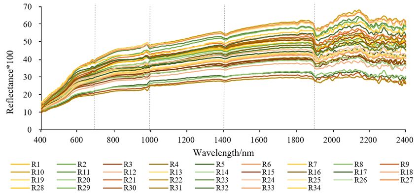
smoothness of the spectra and reduce the noise interference. The indoor reflectance spectral curves of
the topsoil samples (Figure 2) range from 0.1 to 0.7 in the total band. It can be clearly found that the soil
spectral curve has two distinct absorption valleys near the two bands of 1400–1900 nm, and there are
two weak absorption valleys near the 700 nm and 1000 nm bands in virtue of water molecules in the
soil sample vibration frequency generated with the frequency combiner. In the 1950–2400 nm spectra,
the spectra are in a wave form, mainly because of the small amount of moisture in the soil samples
and the moisture absorption in the air. On the whole, the reflectance spectra curves of the soil present
a parabolic pattern, and its reflectance increases with the increase of the wavelength. Among them,
the rising speed is obvious in the range of 400–600 nm, and it is moderately slow in the range of
600–800 nm. After 800 nm, the rise of the spectral reflectance is relatively gentle.Sustainability 2019, 11, 667 7 of 18
Sustainability 2019, 11, x FOR PEER REVIEW 7 of 18
Figure 2.
Figure Soil sample
2. Soil sample reflectance
reflectance curve
curve after
after Savitzky–Golay
Savitzky–Golay (S–G)
(S–G) filtering.
filtering.
3.2. Extraction of Characteristic Bands of SOM, TN, and TC Contents in Soil
3.2. Extraction of Characteristic Bands of SOM, TN, and TC Contents in Soil
The spectral reflectance after S–G filtering is transformed into the first derivative transformation
The spectral reflectance after S–G filtering is transformed into the first derivative transformation
(Figure 3a), first derivative of reciprocal transformation (Figure 3b), second derivative of
(Figure 3a), first derivative of reciprocal transformation (Figure 3b), second derivative of reciprocal
reciprocal transformation (Figure 3c), and first derivative of logarithmic transformation (Figure 3d).
transformation (Figure 3c), and first derivative of logarithmic transformation (Figure 3d). For
For convenience, the reflectance spectrum curve of the No.3 sampling soil is randomly selected
convenience, the reflectance spectrum curve of the No.3 sampling soil is randomly selected for
for observation.
observation.
The band of no.3 soil sample is mainly positive between 400 and 1800 nm after the R0 , (1/R), (lgR)0
differential transformation. It fluctuates between the band of 1800–2400 nm in a large range of positive
and negative fluctuation, and there are more peaks and troughs. (1/R)” differential transformation
amplifies the reflectance rising band of 400–600 nm of the original spectral curve, and multiple peaks
appear. After the differential transformation of (1/R)0 and the (lgR)0 differential transformation, the
weak absorption valleys of 700–1000 nm of the original spectral curve were amplified, and more
peak bands appeared. It can be found that the differential transformation can amplify the subtle
changes in the original spectral curve, which is convenient for further extracting the characteristic
bands corresponding to the SOM, TN, and TC elements in the soil.
Correlation analysis between the SOM, TN, and TC contents of the 34 topsoil samples and the
transformed forms of reflectance spectra was carried out in detail. Finally, the wavelength of the
significant level p < 0.01 was selected as the characteristic band (Table 2).
Viewed from Table 2, it is indicated that the number of characteristic bands extracted from each
differential transformation is not the same. The correlation coefficients between SOM, TN, and TC
contents in soil and the differential transformation are also different. The spectral transformation of
(1/R)0 has the best correlation with the SOM content in soil. There are 13 characteristic bands, which
are respectively 498–501 nm, 1180–1182 nm, 1946 nm, 1947 nm, and 2323–2326 nm. Among them, there
is a positive correlation near the 2324 nm and a negative correlation near the 500 nm band. For the
highest correlation between the soil TN content and (1/R)0 there are 14 characteristic bands, which
are 536 nm, 900 nm, 1177 nm, 1178 nm, 1285–1287 nm, 1977 nm, 2319 nm–2322 nm, 2345 nm, and
2346 nm respectively. It is positively correlated at 2320 nm and negatively correlated at 1170 nm.
For the highest correlation between the soil TC content and (1/R)0 there are 24 characteristic bands:
536–537 nm, 561–562 nm, 619–622 nm, 899–900 nm, 1234–1235nm, 1438–1439 nm, 1795–1796 nm,
1949–1952 nm, 2345–2347 nm, and 2373 nm, in which the positive correlation is presented in the vicinity
of the 2346 nm and negative correlation is presented in the vicinity of the 1951 nm band.Sustainability 2019, 11, x FOR PEER REVIEW 8 of 18
Sustainability 2019, 11, 667 8 of 18
(a) Spectral reflectance after first derivative.
(b) Spectral reflectance after the first derivative of reciprocal.
(c) Spectral reflectance after the second derivative of reciprocal
(d) Spectral reflectance after the first derivative of logarithm.
Figure 3. Spectral reflectance curve after differential transformation.
Figure 3. Spectral reflectance curve after differential transformation.
The band of no.3 soil sample is mainly positive between 400 and 1800 nm after the R’, (1/R),
(lgR)’ differential transformation. It fluctuates between the band of 1800–2400 nm in a large range of
positive and negative fluctuation, and there are more peaks and troughs. (1/R)” differential
transformation amplifies the reflectance rising band of 400–600 nm of the original spectral curve, and
multiple peaks appear. After the differential transformation of (1/R)’ and the (lgR)’ differential
transformation, the weak absorption valleys of 700–1000 nm of the original spectral curve were
amplified, and more peak bands appeared. It can be found that the differential transformation can
amplify the subtle changes in the original spectral curve, which is convenient for further extracting
the characteristic bands corresponding to the SOM, TN, and TC elements in the soil.
Correlation analysis between the SOM, TN, and TC contents of the 34 topsoil samples and the
transformed forms of reflectance spectra was carried out in detail. Finally, the wavelength of the
significant level p < 0.01 was selected as the characteristic band (Table 2).Sustainability 2019, 11, 667 9 of 18
Table 2. Sensitive band deletion of soil organic matter (SOM), total nitrogen (TN), and total carbon
(TC) content.
Sensitive Band nm
Maximum Correlation Minimum Correlation Number
Elements Transformation (p < 0.01)
Band nm R Band nm R
R0 855 0.468 ** 2213 −0.402 * 2 855, 854
498–501, 1180–1182, 1946,
SOM (1/R)0 2324 0.479 ** 500 −0.484 ** 13
1947, 2323–2326
(lgR)0 855 0.441 ** 534 −0.465 ** 3 533, 534, 855
874, 899, 900, 901, 2319,
(1/R)” 900 0.477 ** 1952 −0.425 * 7
2320, 2346
514, 515, 785–790,
R0 1291 0.543 ** 1358 −0.442 * 21 854–856, 1290–1293, 1358,
1359, 1493–1496
TN
496–502, 523–525,
530–534, 1179–1184,
1239–1243, 1268, 1291,
(1/R)0 2325 0.547 ** 500 −0.558 ** 46
1292, 1358–1360,
1426–1428, 1947, 1948,
2323–2327, 2339–2342
536, 900, 1177, 1178,
(1/R)” 2320 0.574 ** 1177 −0.472 ** 14 1285–1287, 1977,
2319–2322, 2345, 2346
786–789, 855, 856, 1181,
1182, 1241, 1242,
(lgR)0 1291 0.502 ** 1359 −0.458 ** 25 1290–1293, 1358–1360,
1494, 1947, 1948,
2324–2326, 2340, 2341
479, 480, 642–644,
689–691, 726–732,
R0 1946 0.538 ** 2368 −0.474 ** 42 785–791, 990–996,
1798–1801, 1943–1948,
TC
2367–2369
494–501, 531–534,
638–644, 696, 697,
1179–1184, 1238–1244,
(1/R)0 1946 0.569 ** 1240 −0.521 ** 49
1799, 1800, 1801, 1930,
1931, 1943–1948,
2340–2342, 2367
536, 537, 561, 562,
619–622, 899, 900, 1234,
(1/R)” 2346 0.579 ** 1951 −0.538 ** 24 1235, 1438, 1439, 1795,
1796, 1949–1952,
2345–2347, 2373
479, 480, 639–644, 696,
697, 728, 785–791, 993,
(lgR)0 1945 0.559 ** 1240 −0.488 ** 37 994, 1239–1242, 1358,
1798–1801, 1943–1948,
2367, 2368
** and *, is significant at the level 0.01 and 0.05%, respectively.
3.3. Model Construction and Accuracy Verification
3.3.1. Hyperspectral Estimation Model of SOM, TN, and TC Content Based on SVM
The total 34 topsoil samples were divided into two groups (24 for the training set, the remaining
10 for the test set). The characteristic band data of 24 soil samples and the corresponding soil SOM, TN,
and TC contents were selected as the input and output of the training set respectively. The variables
for the input and output of the test set were the characteristic band data of 10 soil samples and the
corresponding soil SOM, TN, and TC contents respectively. For example, for the SOM of soil samples
based on the (1/R)0 , the randomly selected 24 samples and the extracted 13 characteristic band data
constituted a 24 × 13 doubt type matrix as the input of the SVM training set. The corresponding soil
organic matter content was composed of 24 × 1 doubt type matrix as the output of the training set.
The remaining 10 samples and the data of the 13 characteristic bands constituted a 10 × 13 doubt
matrix as the input of the test set, while the 10 samples corresponding to the measured SOM content
constituted a 10 × 1 doubt matrix as the output of the test set.Sustainability 2019, 11, 667 10 of 18
Since the input data units were different and some data ranges were relatively large, this would
lead to a too long training time, and the input of different ranges would also affect the accuracy
of the modeling. Therefore, the data of training set and test set were normalized by using the
“mapminmax” function in MATLAB2014b, and then mapped to [0, 1] interval. Its normalization
algorithm is as follows:
x − min
y= (12)
max − min
In the formula, the min is the minimum value and the max is the maximum value in the input
sample set. In the creation and training of the SVM, the type of “−t” kernel function was chosen as the
RBF kernel function. The method of using the grid search cross-validation traversal c and g values
that obtained the optimum parameters of the c and g, “−s” namely the SVM type selection for e-SVR
type and “−p” set the value of the loss function p in the e-SVR type as 0.01. Finally, the “Svmpredict“
function and the trained model are used to predict the effective values of the remaining 10 samples,
and the predicted values are reversely normalized using “mapminmax” function to better restore the
real values. The final model validation accuracy is shown in Table 3.
Table 3. Results of soil SOM, TN and TC contents obtained by support vector machine (SVM).
Estimation model Validation Model
Elements Variable
R2 RMSE R2 RMSE
R0 0.74 ** 0.39 0.72 ** 0.7
(1/R)0 0.68 ** 0.28 0.93 ** 0.23
SOM
(lgR)0 0.89 ** 0.18 0.7 ** 0.34
(1/R)” 0.84 ** 0.32 0.84 ** 0.24
R0 0.74 ** 0.37 0.67 ** 0.26
(1/R)0 0.63 ** 0.31 0.61 ** 0.65
TN
(lgR)0 0.76 ** 0.24 0.71 ** 0.19
(1/R)” 0.87 ** 0.27 0.88 ** 0.17
R0 0.64 ** 0.31 0.7 ** 0.18
(1/R)0 0.57 ** 0.4 0.54 * 0.29
TC
(lgR)0 0.82 ** 0.22 0.63 ** 0.38
(1/R)” 0.86 ** 0.23 0.85 ** 0.26
** and *, is significant at the level 0.01 and 0.05%, respectively.
Table 3 shows that the first-order differential of reciprocal reflectance of soil samples has the
highest accuracy in estimating SOM contents, the predictive determination coefficient R2 is 0.93, and
the predictive root mean square error (RMSE) is 0.23. The second-order differential of reciprocal
reflectance of soil samples has the highest accuracy in estimating soil TN content, the R2 is 0.88 and
RMSE is 0.17. The second order differential estimated soil TC content with the highest accuracy is also
the highest, the R2 is 0.85 and RMSE is 0.26.
3.3.2. Hyperspectral Estimation Model of SOM, TN and TC contents Based on BP Neural Network
The modeling form of the BP neural network is similar to the SVM model. Both training sets and
test sets need to be set in order to facilitate the observation and the accuracy comparison of the two
models. The same test set and training set as the SVM modeling are selected. At the same time, similar
to SVM modeling, both the training set and the test set must be normalized to map them to the [0, 1]
interval. When creating a neural network, the training method selects the gradient descent method,
the number of iterations is set to 1000 times, the training target is set to e−30 , that is, the RMSE of the
training is less than le-30, the number of neurons is set to 10, and the learning rate is set to 0.01. After
the simulation test is the same as the de-normalization and SVM modeling. The final model precision
is shown in Table 4.Sustainability 2019, 11, 667 11 of 18
Table 4. Result of soil SOM, TN and TC contents obtained by back propagation (BP).
Estimation model Validation Model
Elements Variable
R2 RMSE R2 RMSE
R0 0.89 ** 0.26 0.7 ** 0.24
(1/R)0 0.83 ** 0.09 0.87 ** 0.33
SOM
(lgR)0 0.95 ** 0.02 0.63 ** 0.44
(1/R)” 0.66 * 0.06 0.77 ** 0.18
R0 0.85 ** 0.08 0.52 * 0.54
(1/R)0 0.82 ** 0.09 0.53 * 0.6
TN
(lgR)0 0.82 ** 0.04 0.69 ** 0.35
(1/R)” 0.85 ** 0.05 0.79 ** 0.46
R0 0.86 ** 0.13 0.62 ** 0.48
(1/R)0 0.93 ** 0.03 0.43 * 0.52
TC
(lgR)0 0.9 ** 0.04 0.6 ** 0.33
(1/R)” 0.6 * 0.19 0.79 ** 0.38
** and *, is significant at the level 0.01 and 0.05%, respectively.
Table 4 shows that the precision of estimating the SOM content by the first-order differential of
reciprocal reflectance of soil samples is higher, the predictive determinant coefficient R2 is 0.87, and
the prediction RMSE is 0.33. The precision of estimating the soil TN content by the second-order
differential of reciprocal reflectance of soil samples is higher, the R2 is 0.79, and the RMSE is 0.46. At
the same time, the precision of estimating the TC content by the second-order differential of reciprocal
reflectance of soil samples is higher, the R2 is 0.79, and the RMSE is 0.38.
3.3.3. Accuracy Comparison between SVM and BP for Detecting Soil SOM, TN and TC
Figure 4 shows the comparison between the accuracy of SVM and the BP neural network in the
estimation of the soil nutrient content in coastal wetlands. Figure 4a shows the estimation accuracy
of the SOM content. Figure 4b shows the estimation accuracy of the TN content. Figure 4c shows
the estimation accuracy of the TC content. The abscissa represents four different forms of spectral
transformation, the left ordinate represents the value of the determination coefficient R2 , and the right
ordinate represents the value of RMSE.
Viewed from Figure 4, it was indicated that, based on the coefficient of determination R2 and
RMSE evaluation indicators, the accuracy of estimating the SOM and TN content in coastal wetlands by
SVM is better than that of the BP neural network. In order to more intuitively evaluate the prediction
effect of the SVM model, the soil SOM content in the coastal wetland predicted by the SVM model
constructed by spectral transformation (1/R)0 is compared with the measured SOM content (Figure 5a).
The abscissa coordinate was the measured value and the longitudinal coordinate was the predicted
value. Figure 5b shows the comparison of the TN content predicted by the SVM model using spectral
transformation (1/R)” with the measured TN content. Figure 5c is the comparison of the TC content
predicted by the SVM model using spectral transformation (1/R)” with the measured TC content.
It can be seen from Figure 5 that SVM has a high accuracy in predicting SOM, TN, and TC, which are
uniformly distributed near the line y = x.Figure 4 shows the comparison between the accuracy of SVM and the BP neural network in the
estimation of the soil nutrient content in coastal wetlands. Figure 4a shows the estimation accuracy
of the SOM content. Figure 4b shows the estimation accuracy of the TN content. Figure 4c shows the
estimation accuracy of the TC content. The abscissa represents four different forms of spectral
transformation,
Sustainability the
2019, 11, 667left ordinate represents the value of the determination coefficient R , and the12right
2
of 18
ordinate represents the value of RMSE.
(a) Accuracy comparison of BP and SVM models in predicting SOM content.
(b) Accuracy comparison of BP and SVM models in predicting TN content.
(c) Accuracy comparison of BP and SVM models in predicting TC content.
Figure 4. Comparison of modeling accuracy of soil organic matter (SOM), total nitrogen (TN), and
Figure
total 4. Comparison
carbon of modeling accuracy of soil organic matter (SOM), total nitrogen (TN), and
(TC) content.
total carbon (TC) content.
Viewed from Figure 4, it was indicated that, based on the coefficient of determination R2 and
RMSE evaluation indicators, the accuracy of estimating the SOM and TN content in coastal wetlands
by SVM is better than that of the BP neural network. In order to more intuitively evaluate the
prediction effect of the SVM model, the soil SOM content in the coastal wetland predicted by the SVM(Figure 5a). The abscissa coordinate was the measured value and the longitudinal coordinate was the
predicted value. Figure 5b shows the comparison of the TN content predicted by the SVM model
using spectral transformation (1/R)” with the measured TN content. Figure 5c is the comparison of
the TC content predicted by the SVM model using spectral transformation (1/R)” with the measured
TC content. It can be seen from Figure 5 that SVM has a high accuracy in predicting SOM, TN, and
Sustainability 2019, 11, 667 13 of 18
TC, which are uniformly distributed near the line y = x.
(a) SOM content prediction accuracy.
(b) TN content prediction accuracy.
(c) TC content prediction accuracy.
Figure 5. The prediction of soil SOM, TN, and TC content.
Figure 5. The prediction of soil SOM, TN, and TC content
4. Discussion
4. Discussion
4.1. The Characteristics of Reflectance Spectra for Soils in Coastal Wetland
4.1. The Characteristics
It can be seen from of Figure
Reflectance Spectra
2 that for Soilscurves
the spectral in Coastal Wetland
for the 34 naturally-dried soil samples have
greatItsimilarities. However, due to the different SOM, TN,
can be seen from Figure 2 that the spectral curves for the 34 and TCnaturally-dried
content in eachsoil
soil sample,have
samples the
measured spectralHowever,
great similarities. reflectancedue
of soil samples
to the is also
different SOM,different
TN, andin wave peaks, troughs,
TC content andsample,
in each soil reflectance
the
strength, which is the same as the results of Cécile et al. [44]. The spectral reflectance of
measured spectral reflectance of soil samples is also different in wave peaks, troughs, and reflectance the third core
area of Dafeng Elk National Nature Reserve ranges from 0.1 to 0.7. The spectral reflectance curve is
steep near the 400–800 nm, while the reflectance curve of the 800–2400 nm tends to be gentle. There are
two obvious absorption valleys around 1400nm and 1900nm, which is consistent with the results of
most scholars who study the spectral reflectance characteristics of soil [6–9]. Previous studies have
shown that increasing the SOM content in soil will reduce the spectral reflectance of the soil [45].
However, the results of this study showed (Figure 6) that soil sample No. 34 with the highest SOM
content (45.3 mg.kg−1 ) had higher spectral reflectance than the soil sample No. 23 with the lowestarea of Dafeng Elk National Nature Reserve ranges from 0.1 to 0.7. The spectral reflectance curve is
steep near the 400–800 nm, while the reflectance curve of the 800–2400 nm tends to be gentle. There
are two obvious absorption valleys around 1400nm and 1900nm, which is consistent with the results
of most scholars who study the spectral reflectance characteristics of soil [6–9]. Previous studies have
shown that
Sustainability increasing
2019, 11, 667 the SOM content in soil will reduce the spectral reflectance of the soil [45].
14 of 18
However, the results of this study showed (Figure 6) that soil sample No. 34 with the highest SOM
content (45.3 mg.kg−1) had higher spectral reflectance than the soil sample No. 23 with the lowest
SOM −1
SOMcontent
content(7(7mg.kg
mg.kg−1).). It
It may
may bebe due
due to
to the
the fact
factthat
thatthe
thesubtypes
subtypesof oftidal
tidalsaline
salinesoil
soiland
andmeadow
meadow
coastal saline soil in the third core area of Dafeng Elk National Nature Reserve
coastal saline soil in the third core area of Dafeng Elk National Nature Reserve are greatly affected are greatly affected
bybyocean
oceantides,
tides,and
andthe thesalt
saltcontent
contentisisrelatively
relativelyhigh,
high,thus
thusreducing
reducingthe thespectral
spectralreflectance
reflectanceofofthe
the
SOM
SOM content in the soil. Until now, researchers have discovered that the spectral reflectanceofofSOM
content in the soil. Until now, researchers have discovered that the spectral reflectance SOM
ininthe
thecoastal
coastal wetland
wetland soil is significantly
soil is significantlyhigher
higherthan
thanthat
thatofof
thethe non-wetland
non-wetland soils.
soils. ForFor example,
example, Gao
Gao et [15]
et al. al. [15] found
found thatthat
thethe
SOM SOM content
content in Minjiang
in Minjiang Estuary
Estuary wetland
wetland soil
soil was
was directlyproportional
directly proportionalto
tothe
thespectral
spectralreflectance
reflectanceininthe theband
band of
of 600–2500
600–2500 nm. nm. Wang
Wang et et al.
al. [46]
[46] found
foundthat
thatthe
theincreasing
increasingsoil
soil
salinity in the Yellow River delta wetland would also result in a higher spectral
salinity in the Yellow River delta wetland would also result in a higher spectral reflectance. reflectance.
Figure6.6.The
Figure Thespectral
spectralreflectance
reflectanceofofsoil
soilsamples
samplesNo.
No.2323and
andNo.
No.34.
34.
4.2. The Sensitive Bands and Estimation Accuracy for SOM, TN and TC Contents of Coastal Wetland Soil
4.2. The Sensitive Bands and Estimation Accuracy for SOM, TN and TC Contents of Coastal Wetland Soil
After S–G filtering and (1/R)0 transformation, the original spectral reflectance has a high and
After S–G filtering and (1/R)’ transformation, the original spectral reflectance has a high and
negative correlation with the SOM content in soil around 500 nm. The sensitive bands extracted were
negative correlation with the SOM content in soil around 500 nm. The sensitive bands extracted were
498–501 nm, 1180–1182 nm, 1946 nm, 1947 nm and 2323–2326 nm. After (1/R)” transformation,
498–501 nm, 1180–1182 nm, 1946 nm, 1947 nm and 2323–2326 nm. After (1/R)” transformation, it is
it is highly correlated with the soil TN and TC contents. The TN sensitive bands are 536 nm,
highly correlated with the soil TN and TC contents. The TN sensitive bands are 536nm, 900nm,
900 nm, 1177 nm, 1178 nm, 1285–1287 nm, 1977 nm, 2319–2322 nm, 2345 nm and 2346 nm. The TC
1177nm, 1178nm, 1285–1287nm, 1977 nm, 2319–2322 nm, 2345 nm and 2346 nm. The TC sensitivity
sensitivity bands are 536–537 nm, 561–562 nm, 619–622 nm, 899–900 nm, 1234–1235 nm, 1438–1439 nm,
bands are 536–537 nm, 561–562 nm, 619–622 nm, 899–900 nm, 1234–1235 nm, 1438–1439 nm, 1795–
1795–1796 nm, 1949–1952 nm, 2345–2347 nm, and 2373 nm. These bands are different from the SOM
1796 nm, 1949–1952 nm, 2345–2347 nm, and 2373 nm. These bands are different from the SOM
sensitive bands: 362 nm, 392 nm, 422 nm, 437 nm, 537 nm, 652 nm, 702 nm and 1062 nm extracted by
sensitive bands: 362 nm, 392 nm, 422 nm, 437 nm, 537 nm, 652 nm, 702 nm and 1062 nm extracted by
continuous projection method of the collected paddy soil, brick laterite, and loess by Zhang et al. [35].
continuous projection method of the collected paddy soil, brick laterite, and loess by Zhang et al. [35].
This is also different from the TN sensitive bands of 500–900 nm and 1350–1490 nm extracted by
This is also different from the TN sensitive bands of 500–900 nm and 1350–1490 nm extracted by the
the Norris filter and the first-order differential transformation of soil collected by Zhang et al. [47] in
Norris filter and the first-order differential transformation of soil collected by Zhang et al. [47] in the
the middle and eastern China. However, the soils of the Sanjiangyuan region of China collected by
middle and eastern China. However, the soils of the Sanjiangyuan region of China collected by Yang
Yang [48], using differential transformation, are similar to the TC sensitivity bands of 500–900 nm,
[48], using differential transformation, are similar to the TC sensitivity bands of 500–900 nm, 1400–
1400–1500 nm, 1900–2000 nm, and 2200–2300 nm. The reason for the difference in the above research
1500 nm, 1900–2000 nm, and 2200–2300 nm. The reason for the difference in the above research results
results may be the different soil types in the study area. The soil types in the third core area of Dafeng
may be the different soil types in the study area. The soil types in the third core area of Dafeng Elk
Elk National Nature Reserve are mainly tidal flat salt soil and meadow coastal salt soil. These two soil
National Nature Reserve are mainly tidal flat salt soil and meadow coastal salt soil. These two soil
types usually contain between 0.8 and 2.0% salt, and the highest salt content is as much as 4% [49].
types usually contain between 0.8 and 2.0% salt, and the highest salt content is as much as 4% [49].
The spectra reflectance of the soil and the spectral information of SOM, TN, and TC in soil will be
The spectra reflectance of the soil and the spectral information of SOM, TN, and TC in soil will be
further affected by the soil salinity [15].
further affected by the soil salinity [15].
The results of this study indicate that the accuracy of SOM, TN, and TC in soil by SVM is better
than that of the BP neural network, which is consistent with the results of the estimation model
of nitrogen, phosphorus, and potassium in Zhangzhou red soil and Haining green purple mud
constructed by Jiang et al. [50] through least squares support vector machine and BP neural network.
In this study, the SVM estimation model constructed by the (1/R)0 transformation of the spectrum has
the highest accuracy in predicting the SOM content of the coastal wetland soil, R2 is 0.93 and the RMSE
is 0.23. It is higher than the accuracy (R2 = 0.84) of the SOM content in Jianghan Plain predicted bySustainability 2019, 11, 667 15 of 18
Yu et al. [33] by partial least squares regression modeling method. At the same time, it is better than
the prediction accuracy (R2 = 0.83) of the SOM content in Meijiang Township, Suichuan County, Jiangxi
Province constructed by Liu [51] with first-order differential and least squares regression method.
In this study, the SVM estimation model of the TN and TC content in coastal wetland soil constructed
by the (1/R)” transformation of the spectrum, the prediction coefficient R2 is 0.88 and 0.85 respectively,
RMSE is 0.17 and 0.26 respectively. This is better than the prediction accuracy (R2 = 0.832) of the TN
content of the Minjiang Estuary wetland constructed by exponential transformation and unary linear
regression by Gao et al. [15], and is also superior to Yang [48] in predicting the TC content of marsh
soil in the Sanjiangyuan region of China by BP neural network (R2 = 0.81). This indicates that the SVM
model based on the differential transformation form of hyperspectral reflectance has certain feasibility
in predicting SOM, TN, and TC content in coastal wetlands soil, but whether the model can predict the
nutrient content in the coastal wetland soil in other areas needs further verification.
Viewed from the number of soil samples, although the number of samples in this experiment is
only 34, the estimation accuracy of the soil TN content by using the SVM model is higher than that
of the 140 surface soil samples collected by Antonions et al [52]. In addition to the differences in the
study area, another important reason may be the difference in the number of sampling points and the
sampling interval. Therefore, in the future, the effect of the sampling interval of sample points and the
number of samples on the model accuracy should be discussed in depth.
5. Conclusions
In this study, 34 topsoil samples were collected in the coastal wetland and reflectance spectra
of soil samples were measured in a dark room. All of the reflectance spectra were preprocessed by
S–G filtering and then subjected to four differential transformations of R0 , (1/R)0 , (1/R)”, and (lgR)0
respectively. Next, the correlation coefficient was analyzed in order to retrieve the characteristic bands
which were sensitive to soil SOM, TN, and TC contents. The estimation models of soil SOM, TN, and
TC contents in coastal wetland soil were determined based on support vector machine (SVM) and BP
neural network algorithms. The major findings are as follows:
(1) The model accuracy based on SVM in detecting soil SOM, TN and TC contents is significantly
better than that based on the BP neural network.
(2) There is a high correlation between SOM and the reciprocal (1/R)0 of reflectance spectra, the
number of bands with significant correlation (p < 0.01) were 13 and the correlation is the highest
at 500 nm, the correlation coefficient (R) is −0.484. There is a relative high correlation between
TN and the second-order differentials (1/R)” of reflectance spectra. The number of bands
with significant correlation (p < 0.01) was 14, and the highest correlation at 2320 nm is found
with correlation coefficient (R) of 0.574. There is also a high correlation between TC and the
second-order differentials (1/R)” of reflectance spectra. There are 24 bands, which are significantly
correlated (p < 0.01), and the highest correlation at 2346 nm is determined with the correlation
coefficient (R) of 0.579.
(3) The accuracy of the estimation model of SOM based on SVM is the highest, with the prediction
coefficient R2 of 0.93 and RMSE of 0.23 mg kg−1 , respectively.
(4) In the future, the impact of the numbers of soil samples on the accuracy of the estimation model
and root mean square error should be further discussed.
Author Contributions: X.L. and S.Z. conceived and designed the experiment; S.Z. performed the experiments
and analyzed the data; Y.Z. improved the data analysis and supervised the research; S.Z., G.N., and Y.L. drafted
the paper; Y.Z. edited the paper.
Funding: This research was jointly supported by the National Natural Science Foundation of China (No.
41506106), the Key Laboratory for Geo-Environmental Monitoring of Coastal Zone of the National Administration
of Surveying, Mapping and Geo-information (No. GE-2017-003), the Marine Technology Brand Specialty
Construction Project of Jiangsu Province (No. PPZY2015B116), the Pioneer Science and Technology SpecialSustainability 2019, 11, 667 16 of 18
Training Program B (No. XDPB11-01-04) of Chinese Academy of Sciences, and the China-Italy Collaborate Project
for Lunar Surface Mapping (No. 2016YFE0104400).
Conflicts of Interest: The authors declare no conflict of interests.
References
1. Nadi, M.; Golchin, A.; Sedaghati, E.; Shafie, S.; Hosseini fard, S.J.; Füleky, G. Using Nuclear Magnetic
Resonance 1H and 13C in soil organic matter covered by forest. J. Soil Water Conserv. 2017, 21, 83–92.
[CrossRef]
2. Ma, K.; Zhang, Y.; Tang, S.X.; Liu, G. Characteristics of spatial distribution of soil total nitrogen in Zoigen
alpine wetland. Chin. J. Ecol. 2016, 35, 1988–1995.
3. Jauss, V.; Sullivan, P.; Lehmann, J.; Sanderman, J.; Daub, M. Alternative modelling approaches for estimating
pyrogenic carbon, soil organic carbon and total nitrogen in contrasting ecoregions within the United States.
Geophys. Res. Abstr. 2017, 19, 497.
4. Lu, X.; Lin, Y.L.; Wu, Y.N.; Gu, Y.; Zhao, Q.; Zhang, X. Spatial Distribution Characteristics of Soil Physical
and Chemical Properties in Milu National Nature Reserve of Coastal Wetland. Trans. Oceanol. Limnol. 2018,
4, 74–81.
5. Vohland, M.; Emmerling, C. Determination of total soil organic C and hot water-extractable C from VIS-NIR
soil reflectance with partial least squares regression and spectral feature selection techniques. Soil Sci. 2011,
62, 598–606. [CrossRef]
6. Wu, D.; Shi, H.; Wang, S.J.; He, Y.; Bao, Y.D.; Liu, K.S. Rapid prediction of moisture content of dehydrated
prawns using online hyperspectral imaging system. Anal. Chim. Acta 2012, 726, 57–66. [CrossRef] [PubMed]
7. Wu, G.F.; He, Y. Application of Wavelet Threshold Denoising Model to Infrared Spectral Signal Processing.
Spectrosc. Spectr. Anal. 2009, 29, 3246–3249.
8. Radim, V.; Radka, K.; Aleš, K.; Luboš, B. Simple but efficient signal pre-processing in soil organic carbon
spectroscopic estimation. Geoderma 2017, 298, 46–53.
9. Shen, Y.; Zhang, X.P.; Liang, A.Z.; Shi, X.H.; Fan, R.Q.; Yang, X.M. Multiplicative scatter correction and step
is regression to build NIRS model for analysis of soil Organic Carbon content in black soil. Syst. Sci. Compr.
Stud. Agric. 2010, 26, 174–180.
10. Hu, T.; Qi, K.; Hu, Y. Using vis-nir spectroscopy to estimate soil organic content. In Proceedings of the
IGARSS 2018—2018 IEEE International Geoscience and Remote Sensing Symposium, Valencia, Spain, 22–27
July 2018.
11. Chen, H.Y. Hyperspectral Estimation of Major Soil Nutrient Content. Ph.D. Thesis, Shandong Agricultural
University, Shandong, China, 2012.
12. Sun, W.; Li, X.; Niu, B. Prediction of soil organic carbon in a coal mining area by Vis-NIR spectroscopy.
PLoS ONE 2018, 13. [CrossRef]
13. Chen, H.Y.; Zhao, G.X.; Li, X.C.; Zhu, X.C.; Sui, L.; Wang, Y.J. Hyperspectral estimation of soil organic matter
content based on wavelet transformation. Chin. J. Appl. Ecol. 2011, 22, 2935–2942.
14. Sorenson, P.T.; Small, C.; Tappert, M.C.; Quideau, S.A.; Drozdowski, B.; Underwood, A.; Janzd, A. Monitoring
organic carbon, total nitrogen, and pH for reclaimed soils using field reflectance spectroscopy. Can. J. Soil Sci.
2017, 97, 241–248. [CrossRef]
15. Gao, D.Z.; Zeng, C.S.; Zhang, W.L.; Liu, Q.Q.; Wang, Z.P.; Chen, Y.T. Estimating of soil total nitrogen
concentration based on hyperspectral remote sensing data in Minjiang River estuarine wetland. Chin. J. Ecol.
2016, 35, 952–959.
16. Wu, M.Z.; Li, X.M.; Sha, J.M. Spectral Inversion Model for Prediction of Red Soil Total Nitrogen Content in
Subtropical Region (Fuzhou). Spectrosc. Spectr. Anal. 2013, 33, 3111–3115.
17. He, Y.; Xiao, S.; Nie, P.; Dong, T.; Qu, F.; Lin, L. Research on the Optimum Water Content of Detecting Soil
Nitrogen Using Near Infrared Sensor. Sensors 2017, 17, 2045. [CrossRef]
18. Zhou, X.B.; Zhao, J.W. Methods of Characteristic Wavelength Region and Wavelength Selection Based on
Genetic Algorithm. Acta Opt. Sin. 2007, 27, 1316–1321.
19. Zhang, Y. Research on Spectral Region Selection of Near Infrared Spectra Based on Genetic Algorithm.
In Proceedings of the 2017 9th International Conference on Intelligent Human-Machine Systems and
Cybernetics (IHMSC), Hangzhou, China, 26–27 August 2017.You can also read