Non-Exhaustive Learning Using Gaussian Mixture Generative Adversarial Networks
←
→
Page content transcription
If your browser does not render page correctly, please read the page content below
Non-Exhaustive Learning Using Gaussian
       Mixture Generative Adversarial Networks

                      Jun Zhuang [0000−0002−7142−2193]
                   Mohammad Al Hasan [0000−0002−8279−1023]

    Indiana University-Purdue University Indianapolis, Indianapolis, IN, 46202, USA
                          junz@iu.edu, alhasan@iupui.edu

        Abstract. Supervised learning, while deployed in real-life scenarios, of-
        ten encounters instances of unknown classes. Conventional algorithms
        for training a supervised learning model do not provide an option to
        detect such instances, so they miss-classify such instances with 100%
        probability. Open Set Recognition (OSR) and Non-Exhaustive Learning
        (NEL) are potential solutions to overcome this problem. Most existing
        methods of OSR first classify members of existing classes and then iden-
        tify instances of new classes. However, many of the existing methods
        of OSR only makes a binary decision, i.e., they only identify the exis-
        tence of the unknown class. Hence, such methods cannot distinguish test
        instances belonging to incremental unseen classes. On the other hand,
        the majority of NEL methods often make a parametric assumption over
        the data distribution, which either fail to return good results, due to
        the reason that real-life complex datasets may not follow a well-known
        data distribution. In this paper, we propose a new online non-exhaustive
        learning model, namely, Non-Exhaustive Gaussian Mixture Generative
        Adversarial Networks (NE-GM-GAN) to address these issues. Our pro-
        posed model synthesizes Gaussian mixture based latent representation
        over a deep generative model, such as GAN, for incremental detection
        of instances of emerging classes in the test data. Extensive experimental
        results on several benchmark datasets show that NE-GM-GAN signifi-
        cantly outperforms the state-of-the-art methods in detecting instances
        of novel classes in streaming data.

        Keywords: Open set recognition · Non-exhaustive learning.

1     Introduction
Numerous machine learning models are supervised, relying substantially on la-
beled datasets. In such datasets, the labels of training instances enable a su-
pervised model to learn the correlation between the labels and the patterns
in the features, thus helping the model to achieve the desired performance in
different kinds of classification or recognition tasks. However, many realistic
machine learning problems originate in non-stationary environments where in-
stances of unseen classes may emerge naturally. The presence of such instances
weakens the robustness of conventional machine learning algorithms, as these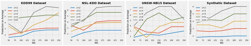
2      Jun Zhuang, Mohammad Al Hasan

algorithms do not account for the instances from unknown classes, either in
the train or the test environments. To overcome this challenge, a series of re-
lated research activities has become popular in recent years; examples include
anomaly detection (AD) [13,15,27,34], few-shot learning (FSL) [12,25], zero-shot
learning (ZSL) [21,29], open set recognition (OSR) and open-world classification
(OWC) [1,2,4,5,8,11,14,17,19,20,23,26,30,31]. Collectively, each of these works
belongs to one of the four different categories [6], differing on the kind of in-
stances observed by the model during train and test. If L refers to labeling and
I refers to self-information (e.g., semantic information in image dataset), the
categories C can be denoted as the Cartesian product of two sets L and I, as
shown below:
                      C = L × I = {(l, i) : l ∈ L & i ∈ I},                   (1)
both L and I have two elements: known (K) and unknown (U). Thus, there are
four categories in C: (K, K), (K, U), (U, K), (U, U). For example, (U, U) refers
to the learning problem in which instances belonging to unknown classes having
no self-information.
    Conventional supervised learning task belongs to the first category, as for
such a task all instances in train and test datasets belong to (K, K). The anomaly
detection (AD) task, a.k.a. one-class classification or outlier detection, detects
a few (U, U) instances from the majority of (K, K) instances; for AD, the (U,
U) instances may only (but not necessary) exist in the test set. FSL and ZSL
are employed to identify (U, K) instances in the test set. The main difference
between FSL and ZSL is that the training set of FSL contains a limited number
of (U, K) instances while for the case of ZSL, the number of (U, K) instances
in the train set is zero. In other words, ZSL identifies (U, K) instances in the
test set only by associating (K, K) instances with (U, K) instances through self-
information. Finally, works belonging to open set recognition (OSR) identify (U,
U) instances in the test set. These works are the most challenging; unlike AD,
whose objective is to detect only one class (outlier), OSR handles both (K, K)
and (U, U) in the test set. Similar to OSR, OWC also incrementally learns the
new classes and rejects the unseen class. Nevertheless, most existing methods of
OSR or OWC do not distinguish the test instances among incremental unseen
classes, which is more close to the realistic scenario. The scope of our work falls
in the OSR category which only deals with (K, K) and (U, U) instances. In
Table 1, we present a summary of the discussion of this paragraph.
    Some works belonging to OSR have also been referred as Non-Exhaustive
Learning (NEL). The term, Non-Exhaustive, means that the training data does
not have instances of all classes that may be expected in the test data. The
majority of early research works of NEL employ Bayesian methods with Gaussian
mixture model (GMM) or infinite Gaussian mixture model (IGMM) [24, 33].
However, these works suffer from some limitations; for instance, they assume
that the data distribution in each class follows a mixture of Gaussian, which
may not be true in many realistic datasets. Also, in the case of GMM, its ability
to recognize unknown classes depends on the number of initial clusters that it
uses. IGMM can mitigate this restriction by allowing cluster count to grow on the
Non-Exhaustive Gaussian Mixture Generative Adversarial Networks 3
Table 1. The Background of Related Tasks (Conv. for Conventional Method)
Tasks Training Set Testing Set GOAL
Conv. (K, K) (K, K) Supervised learning with (K, K)
AD (K, K) w./wo. outliers (K, K) w. outliers Detect outliers
FSL (K, K) w. limited (U, K) (U, K) Identify (U, K) in test set
ZSL (K, K) w. self-info. (U, K) Identify (U, K) in test set
OSR (K, K) (K, K) & (U, U) Distinguish (U, U) from (K, K)
NEL (K, K) (K, K) & (U, U) Incrementally learn (U, U)
fly, but the inference mechanism of IGMM is time-consuming, no matter what
kind of sampling method it uses for inferring the probabilities of the posterior
distribution.
To address these issues, in this work we propose a new non-exhaustive learn-
ing model, Non-exhaustive Gaussian mixture Generative Adversarial Networks
(NE-GM-GAN), which synthesizes the Bayesian method and deep learning tech-
nique. Comparing to the existing methods for OSR, our proposed method has
several advantages: First, NE-GM-GAN takes multi-modal prior as input to
better fit the real data distribution; Second, NE-GM-GAN can deal with class-
imbalance problem with end-to-end offline training; Finally, NE-GM-GAN can
achieve accurate and robust online detection on large sparse dataset while avoid-
ing noisy distraction. Extensive experiments demonstrate that our proposed
model has superior performance over competing methods on benchmark datasets.
The contribution of this paper can be summarized as follows:
• We propose a new model for non-exhaustive learning, namely NE-GM-
GAN, which can detect novel classes in online test data accurately and defy the
class-imbalance problem effectively.
• NE-GM-GAN integrates Bayesian inference with the distance-based and
the threshold-based method to estimate the number of emerging classes in the
test data. It also devises a novel scoring method to distinguish the UCs (unknown
classes) from KCs (known classes).
• Extensive experiments on four datasets (3 real and 1 synthetic) demonstrate
that our model is superior to existing methods for accurate and robust online
detection of emerging classes in streaming data.
2 Related Work
Anomaly detection (AD) basically can be divided into two categories, conven-
tional methods, and deep learning techniques. Majority of conventional meth-
ods widely focus on distance-based approaches [15,28], reconstruction-based ap-
proaches [9], and unsupervised clustering. Deep learning techniques usually in-
clude autoencoder and GAN. An autoencoder identifies the outlier instances
through reconstruction loss [34]. GAN has also been used as another means for
computing reconstruction loss and then identifying anomalies [27,32]. In our ap-4 Jun Zhuang, Mohammad Al Hasan
proach, we use bi-directional GAN (BiGAN) with multi-modal prior distribution
to improve the performance of UCs extraction.
AD mainly detects one class of anomalies whereas realistic data often con-
tains multiple UCs. OSR is the right technique that solves this kind of problem.
According to [6], OSR models are categorized into two types, discriminative and
generative. The first type includes SVM-based methods [26] and distance-based
method [1, 2]. A collection of recent OSR works venture towards the generative
direction [4, 11, 19, 31]. A subset of OSR methods, named NEL, mainly employ
Bayesian methods, such as infinite Gaussian mixture model (IGMM) [24] to
learn the UCs. For example, Zhang et al. [33] use a non-parametric Bayesian
framework with different posterior sampling strategies, such as one sweep Gibbs
sampling, for detecting novel classes in online name disambiguation. However,
IGMM-type methods can only handle small datasets that follow Gaussian distri-
bution. To address this issue, we propose a novel algorithm that can achieve high
accuracy on the large sparse dataset, which does not necessarily follow Gaussian
distribution.
3 Background
Generative Adversarial Networks (GAN). Vanilla GAN [7] consists of two
key components, a generator G, and a discriminator D. Given a prior distribution
Z as input, G maps an instance z ∼ Z from the latent space to the data space
as G(z). On the other hand, D attempts to distinguish a data instance x from a
synthetic instance G(z), generated by G. We use the terminology pZ (z) to denote
that z is a sampled instance from the distribution Z. The training process is set
up as if G and D are playing a zero-sum game, a.k.a. minimax game; G tries
to generate the synthetic instances that are as close as possible to actual data
instances; on the other hand, D is responsible for distinguishing the real instances
from the synthetic instances. In the end, GAN converges when both G and D
reach a Nash equilibrium; at that stage, G learns the data distribution and is
able to generate data instances that are very close to the actual data instances.
The objective function of GAN can be written as follows:
min max V (D, G) = E [log D(x)] + E [log(1 − D(G(z)))] (2)
G D x∼X z∼Z
where X is the distribution of x and Z is the distribution from which G samples.
Bidirectional Generative Adversarial Networks (BiGAN). Besides
training a generator G, BiGAN [10] also trains an encoder E, that maps real
instances x into latent feature space E(x). Its discriminator D takes both x and
pZ (z) as input in order to match the joint distribution pG (x, z) and pE (x, z).
The objective function of BiGAN can be written as follows:
min max V (D, E, G) = E [log D(x, E(x))] + E [log(1 − D(G(z), z))] (3)
G,E D x∼X z∼Z
The objective function achieves the global minimum if and only if the distribution
of both generator and encoder matches., i.e., pG (x, z) = pE (x, z).Non-Exhaustive Gaussian Mixture Generative Adversarial Networks 5
4 Methodology
In this paper, we propose a novel model, Non-Exhaustive Gaussian Mixture Gen-
erative Adversarial Networks (NE-GM-GAN) for online non-exhaustive learning.
The whole process is displayed in Figure 1. Given a training set Xtrain with k0
KCs, in the training step (offline), the proposed NE-GM-GAN employs a bidi-
rectional GAN to train its encoder E and generator G, by matching the joint
distribution of encoder (X, Z) with the same of the generator. Note that the
prior distribution Z of G is a multi-modal Gaussian (shown as Gaussian clusters
on the top-middle part of the figure). After training, the generator and encoder
of the GAN can take z and x as input and generate G(z) and E(x) as output,
respectively.
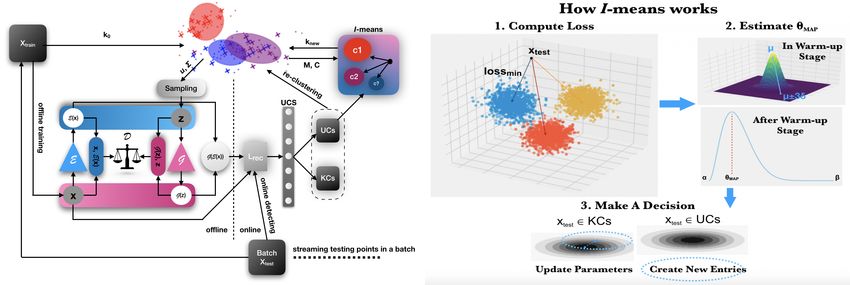
Fig. 1. The Model Architecture of NE-GM-GAN (Left-hand Side) and The Workflow
of I-means in Algorithm (2) (Right-hand Side)
The test step (online) shown on the right side of the model architecture and it
is run on a batch of input instances, Xtest . For all data instance from a batch (say,
x is one such instance), NE-GM-GAN computes the U CS(x) (unknown class
score) of all instances in that batch; UCS score is derived from the reconstruction
loss Lrec = |x−G(E(x))|. Using this score, the instances of a batch are partitioned
into two groups: KCs and UCs. Elements in KCs belong to the known class,
whereas the elements in UCs are potential UC instances. Using instances of UCs
group, the model estimates the number of emerging class, knew . After estimation,
the model updates the prior of the G by adding the number of new classes knew
to k0 as shown in the top right part of the model architecture. The GMM is
then retrained for clustering both KCs and UCs. At this stage, the online test
process for one test batch is finished.
In subsequent discussion, Xtrain ∈ Rr×d is considered to be training data,
containing r data instances, each of which is represented as a d-dimensional
vector. K is the total number of known classes in Xtrain . Xtest is test data that
may contain instances of KCs and also instances of UCs. The dimensionality of
latent space is denoted by p.6 Jun Zhuang, Mohammad Al Hasan
Offline Training: Computing Multi-modal Prior Distribution
In the vanilla form, generators of both GAN and BiGAN has a unimodal dis-
tribution as prior; in other words, the random variables pZ (z) is an instance
from a unimodal distribution. Enlightened by [16], in this paper, we consider
a multi-modal distribution as prior since this prior can better fit the real-life
distribution of multi-class datasets. Thus,
K
X
pZ (z) = α{k} · pk (z) (4)
k=1
We assume that the number of initial clusters in the Gaussian distribution
matches with the number of known classes (K) in Xtrain . α{k} is the mixing
parameter, pk (z) denotes the multivariate Normal distribution N (u{k} , Σ {k} ),
where u{k} and Σ {k} are mean vector and co-variance matrix, respectively.
The model assumes that the number of instances and the number of known
classes in the training set are given at the beginning. During training (offline),
the parameters u{k} and Σ {k} of each Gaussian cluster is learned by GMM and
they are used as the sampling distribution of the latent variable for generating
the adversarial instances. Suggested by [16], we also use the re-parameterization
trick in this paper. Instead of sampling the latent variable z ∼ N (u{k} , Σ {k} ),
the model samples z = A{k} + u{k} , where ∼ N (0, I), A ∈ Rp×p , u{k} ∈ Rp .
In this scenario, u(z) = u{k} and Σ(z) = A{k} A{k}T .
Similar to [10], the GM-GAN (Gaussian Mixture-GAN) learning proceeds
as follows. The model takes sampled instance z, sampled from the Gaussian
multi-modal prior and a real instances x as input. Generator G attempts to map
this sampled pZ (z) to data space as G(z). Encoder E maps real instances x into
latent feature space as E(x). Discriminator D takes both pZ (z) and x as input
for matching their joint distributions. After the model converges, theoretically,
G(z) ∼ x and E(x) ∼ pZ (z). Note that NE-GM-GAN encodes Xtrain for offline
training. To do so, GMM takes encoded Xtrain as input and then generates
encoded u and Σ.
Extracting Potential Unknown Class
UC extraction of NE-GM-GAN is an online process that works on unlabeled
data. During online detection, the model assumes that the test instance x is
coming in a batch of the test set Xtest ∈ Rb×d , where b is batch size and d
is the dimension of feature space. Unlike [10], whose purpose is to generate
the fake images as real as possible, our model aims at extracting the UC as
accurately as possible. More specifically, our model generates the reconstructed
instance G(E(x)) at first and then computes the reconstruction loss between x
and G(E(x)). This step returns a size-b 1-D vector, consisting of reconstruction
losses of the b points in the current batch, which is defined below:
Lrec = kx − G(E(x))k (5)
To distinguish the UC from KC in each test batch, we propose a metric,
unknown class score, in short, U CS; the larger the score for an instance, theNon-Exhaustive Gaussian Mixture Generative Adversarial Networks 7
more likely that the instance belongs to an unknown class. To compute U CS of
a test instance x, NE-GM-GAN first computes, for each KC (out of K KCs), a
baseline reconstruction loss, which is equal to the median of reconstruction losses
of all train objects belonging to that known class. Then, U CS of x is equal to the
minimum of the differences between x’s reconstruction loss and each of the K
baseline reconstruction losses. The pseudo-code of U CS computation is shown
in Algorithm 1.
The intuition of U CS function is that GAN models instances of KCs with
smaller reconstruction loss than the instances of UCs, but different known classes
may have different baseline reconstruction loss, so we want an unknown class’s
reconstruction loss larger than the worst loss among all the KCs. This mechanism
is inspired by [32]. Nevertheless, unlike [32], which assumes the prior as unimodal
distribution and the UC must be far away from KC, our approach considers a
multi-modal prior. After computing the U CS, the model extracts the potential
UC from KC with a given threshold. For online detection, the threshold for the
first test batch is empirically given whereas subsequent thresholds are decided
by the percentage of UCs from previous test batches. Note that, the UCs objects
may belong to multiple classes, but the model has no knowledge yet about the
number of classes.
Algorithm 1: U CS for multi-modal prior
Input: Matrix Xtrain ∈ Rr×d and Xtest ∈ Rb×d
1 Compute Ltest (xtest ) with Equation (5);
2 for i ← 1 to b do
3 for k ← 1 to K do
4 Compute Ltrain (xtrain ){k} with Equation (5);
5 Select the median of Ltrain (xtrain ){k} ;
{k}
6 U CS(xtest ){k} = Ltest (xtest ){i} − Ltrain (xtrain )median ;
7 end
{i}
8 U CSmin = min U CS(xtest ){1} , ..., U CS(xtest ){K} ;
9 end
{1} {b}
10 U CS = [U CSmin , ..., U CSmin ];
b×1
11 return Vector U CS ∈ R
Estimating The Number of Emerging Class
The previous extraction only extracts potential UCs. In practice, a small num-
ber of anomalous KC instances may be selected as UC instances. So, we use a
subsequent step that distinctly identifies instances of unknown classes together
with the number of UC and their parameters (mean, and covariance matrix of
each of the UCs). We name this step as Infinite Means (I-means); the name
reflects the fact that the number of unknown classes can increase as large as
needed based on the test instances. Using I-means, a test instance is assigned to8 Jun Zhuang, Mohammad Al Hasan
a new class if it is positioned far from the mean of all the KCs, and discovered
novel classes prior to seeing that instance. To achieve this, for i-th test instance
{i} {k}
xtest , as shown in Equation (6), I-means computes the distance Lµ between
{i}
xtest and the mean vector µ{k} for the k-th KC and then selects the minimum
of these values as lossmin in Equation (7).
{i}
L{k}
µ = kxtest − µ{k} k, ∀k ∈ [1..K] (6)
lossmin = min Lµ{1} , Lµ{2} , ..., L{K}
µ , idx = arg min L{1} {2} {K}
µ , Lµ , ..., Lµ (7)
{i}
A small value of lossmin indicates that xtest may potentially be a member of
{i}
class idx; on the other hand, a large value lossmin indicates that xtest possibly
belongs to a UC. To make the determination, we use a Bayesian approach, which
dynamically adjusts the probability that a test point that is closest to cluster
idx’s mean vector belongs to cluster idx or not. The process is described below.
{i}
For a test instance, xtest for which idx = k, the binary decision whether the
instance belongs to k-th existing cluster or an emerging cluster follows Bernoulli
distribution with parameter θk , which is modeled by using a Beta prior with
parameter αk , and βk , where αk , βk ≥ 1 and θk = αkα+β k
k
. The value of αk and
βk are updated using Bayes rule. Based on the Bayes’ theorem, the posterior
{i}
distribution p(θk |xtest ), where θk ∈ [0, 1], is proportional to the prior distribution
{i}
p(θk ) multiplied by the likelihood function p(xtest |θk ):
{i} {i}
p(θk |xtest ) ∝ p(xtest |θk ) · p(θk ) (8)
{i}
The posterior p(θk |xtest ) in Equation (8) can be re-written as following:
{i}
p(θk |xtest ) ∝ θkαk0 (1 − θk )βk0 · θkαk −1 (1 − θk )βk −1
= θkαk0 +αk −1 · (1 − θk )βk0 +βk −1 (9)
= beta(θk |αk0 + αk , βk0 + βk )
As the test instances are coming in streaming fashion, for any subsequent test
{i}
instance for which idx = k, the posterior p(θk |xtest ) will act as prior for the
next update. For the very first iteration, αk0 and βk0 are shape parameters of
beta prior, which we learn in a warm-up stage. In the warm-up stage, we apply
the three-sigma rule to compute the beta priors, αk0 , and βk0 . Each test point
in the warm-up stage, for which idx = k, contributes a count of 1 to αk0 if
the point is further than 3 standard deviation away from the mean, otherwise
it contributes a count of 1 to βk0 . After the warm-up stage, we employ the
Maximum-A-Posteriori (MAP) estimation to obtain the θM APk at which the
{i}
posterior p(θk |xtest ) reaches its maximum value. According to the property of
beta distribution, the θM APk is most likely to occur at the mean of posterior
{i}
p(θk |xtest ). Thus, we can estimate the θM APk by:
{i} αk0 + αk
θM APk = arg max p(θk |xtest ) = (10)
θk αk0 + αk + βk0 + βkNon-Exhaustive Gaussian Mixture Generative Adversarial Networks 9
After estimating the θM APk by Equation (10), I-means makes a cluster mem-
{i}
bership decision for each xtest based on θM APk . This decision simulates the
Bernoulli process, i.e., among the test instances which are close to the k-th clus-
ter, approximately θM APk fraction of those will belong to the emerging cluster,
whereas the remaining (1−θM APk ) fractions of such instances will belongs to the
k-th cluster. After each decision, corresponding parameters will be updated. If
{i} {i}
xtest is clustered as a member of KC {k} , we update the parameters µk ∈ R1×d ,
{i}
σk ∈ Rd×d of the k-th cluster by Equation (11) and Equation (12), respectively.
{i}
The shape parameter βk is increased by 1. Otherwise, if xtest is considered as a
member of UC, the shape parameter αk , knew are increased by 1, and the mean
{i}
and covariance matrix of this new class are initialized by assigning current xtest
{i}
as new mean vector and creating a zero vector with the same shape of xtest as
new standard deviation vector.
{i} {i−1}
{i} {i−1} xtest − µk
µk = µk + (11)
i
s
{i}
{i} {i−1}
{i} {i−1}
{i} {i}
{i} vk
vk = vk + xtest − µk xtest − µk , σk = (12)
(i − 1)
The entire process of this paragraph is summarized I-means in Algorithm 2.
Table 2. Statistics of Datasets (#Inst. denotes the number of instances; #F. denotes
to the number of features after one-hot embedding or dropping for network intrusion
dataset; #C. denotes to the number of Classes.)
Dataset #Inst. #F. #C. Selected UCs
KDD99 494,021 121 23 neptune, normal, back, satan, ipsweep,
portsweep, warezclient, teardrop
NSL-KDD 148,517 121 40 neptune, satan, ipsweep, smurf, portsweep,
nmap, back, guess passwd
UNSW-NB15 175,341 169 10 generic, exploits, fuzzers, DoS, reconnaissance,
analysis, backdoor, shellcode
Synthetic 100,300 121 16 No.3, 4, 5, 6, 7, 8, 9, 10
5 Experiments
In this section, we show experimental results for validating the superior per-
formance of our proposed NE-GM-GAN over different competing methods for
multiple capabilities. Firstly, we compare the performance of potential UCs ex-
traction. Furthermore, we compare the estimation of the number of distinct10 Jun Zhuang, Mohammad Al Hasan
Algorithm 2: Infinite Means (I-means)
Input: Testing batch Xtest ∈ Rb×d , mean matrix, co-variance matrix
1 for all x{i} ∈ Xtest do
2 for all µ{k} ∈ M do
{k}
3 Compute Lµ by Equation (6);
4 end
5 Get the index, idx, of minimum loss by Equation (7);
6 if warm-up stage then
7 Select beta prior αidx0 and βidx0 based on Three-sigma Rule;
8 end
9 else
10 Estimate the θM APk by Equation (10);
11 end
12 if Uniform (0, 1) ≤ θM APk then
13 Update corresponding µ and σ by Equation (11) and Equation (12);
14 βidx ← βidx + 1;
15 end
16 else
17 αidx ← αidx + 1;
18 knew ← knew + 1;
19 end
20 end
21 return The number of new emerging clusters knew
unknown classes. Finally, we show some experimental results for studying the
effect of user-defined parameters on the algorithm’s performance.
Dataset. We evaluate NE-GM-GAN on four datasets. Three of the datasets
are real-life network intrusion datasets and the remaining one is a synthetic
dataset. The network intrusion is very common for non-exhaustive classification
because attackers constantly update their attack methods, so the classification
model must adapt to novel class scenarios. The datasets are: (1) KDD Cup 1999
network intrusion dataset (KDD99), which contains 494,021 instances and 41
features with 23 different classes. One of the class represents “Normal” activity
and the rest 22 represent various network attacks; (2) NSL-KDD dataset (NSL-
KDD) [3], which is also a network intrusion dataset built by filtering some
records from KDD99; (3) UNSW-NB15 dataset (UNSW-NB15) [18], which
hybridizes real normal network activities with synthetic attack; (4) Synthetic
dataset (Synthetic), which contains non-isotropic Gaussian clusters. Many of
the features in the intrusion datasets are categorical or binary, so we employ
one-hot embedding for such features. We also drop some columns which are
redundant or whose values are almost zero or missing along the column. After
that, we select eight of the classes as unknown classes (UCs) for each dataset.
The test set is constructed from two parts. The first part is randomly sampled
20% of KCs instances and the second part is all the instances of the UCs. Rest
80% of KC instances are left for the training set. In the synthetic dataset, noisesNon-Exhaustive Gaussian Mixture Generative Adversarial Networks 11
are injected into Gaussian clusters, each cluster representing a class. The injected
noise is homocentric to the corresponding normal class but with a larger variance.
The detailed statistics of the datasets are provided in Table 2.
Competing Methods. The performance of UCs extraction is evaluated with
three competing methods, AnoGAN [27], DAGMM [34], and ALAD [32]. AnoGAN
is the first GAN-based model for UC detection. Similarly, ALAD is another
GAN-based model, which uses reconstructed errors to determine the UC. In
contrast, DAGMM implements the autoencoder for the same task instead. The
experimental setting follows [32] for this experiment. On the other hand, the ca-
pability of estimating the number of new emerging classes is compared against
two competing methods, X-means [22], and IGMM [24, 33]. X-means is a classi-
cal distance-based algorithm that can efficiently search the data space without
knowing the initial number of clusters. On the contrary, IGMM is a Bayesian
mixture model which uses the Dirichlet process prior and Gibbs sampler to ef-
ficiently identify new emerging entities. This experiment uses one sweep Gibbs
sampler for IGMM [33]. For IGMM, we select the tunable parameters as fol-
lowing; h = 10, m = h + 100, κ = 100 and α = 100, which is identical to the
parameter values in [33]. Both models can return the number of online classes
as NE-GM-GAN does, so they are selected as competing methods.
Evaluation Metrics. We use an external clustering evaluation metric, such
as F1-score, to evaluate the performance of UCs extraction. For evaluating the
prediction of the number of UCs (a regression task), we propose a new met-
ric, Symmetrical R-squared (S-R2 ). To obtain this, the root mean square error
(RM SE) for both NE-GM-GAN and a competing method are computed and
plugged into Equation 13. S-R2 ∈ [-1, 1] gets more close to 1 if NE-GM-GAN
defeats the competing method. On the contrary, its value will become more close
-1. S-R2 is exactly equal to 1 when the proposed model gets perfect prediction
while the competing method doesn’t. S-R2 is zero when both methods have
similar performance. The motivation to propose a new metric rather than using
R-squared (R2 ) is that R2 would be less distinctive if two methods get much
worse predictions because of using mean square error (M SE) inside. Besides,
baseline sometimes achieves better performance, but R2 cannot reflect this sce-
nario as its range is from negative infinity to positive one.
RM SEm
1 − , RM SEm < RM SEbl
RM SEbl
S-R2 = (13)
RM SEbl
− 1, RM SEm > RM SEbl
RM SEm
where RM SEm and RM SEbl denote the RM SE of our model and baseline
model, respectively.
The Capability of Unknown Class Extraction. In Table 3, we show the
F1-score values of NE-GM-GAN and the competing methods for detecting the
unknown class instances (the best results are shown in bold font). The result is
computed by running each model 10 times and then taking the average. Out of
the four datasets, NE-GM-GAN has the best performance in three with a healthy12 Jun Zhuang, Mohammad Al Hasan
margin over the second-best method. In the largest dataset, our model received a
0.99 F1-score, a very good performance considering the fact that unknown class
instances are assembled from 8 different classes. Only in the NSL-KDD dataset,
NE-GM-GAN came out as the second-best. The performance of the other three
models is mixed without a clear winner. One observation is that all the methods
perform better on the larger dataset (KDD99).
To understand NE-GM-GAN’s performance further, we perform an ablation
study by switching the prior, as shown in Table 4. As we can see Gaussian multi-
modal prior used in NE-GM-GAN is better suited than Unimodal prior generally
used in traditional GAN. For all datasets multi-modal prior has 1% to 2% better
F-score. A possible reason is that multi-modal prior is more closer to the real
distribution of the training data.
Table 3. The F1-score of Four Models for UCs Extraction
Data NE-GM-GAN AnoGAN DAGMM ALAD
KDD99 0.99 0.87 0.97 0.94
NSL-KDD 0.75 0.68 0.79 0.73
UNSW-NB15 0.57 0.49 0.53 0.51
Synthetic 0.74 0.51 0.70 0.56
Table 4. F1 Score from Our Proposed Model by Using Different Prior
Prior KDD99 NSL-KDD UNSW-NB15 Synthetic
Unimodal 0.98 0.74 0.55 0.72
Multi-modal 0.99 0.75 0.57 0.74
The Estimation of The Number of New Classes. In this experiment, we
compare NE-GM-GAN against two competing methods on all four datasets.
To extend the scope of experiments, we vary the number of unknown classes
from 2 to 6 by choosing all possible combinations of UCs and build multiple
copies of one dataset and report performance results over all those copies. The
motivation of using a combination of different UCs is to validate the robustness of
the methods against varying numbers of UC counts. The result is shown in Table
5 using S-R2 metric discussed earlier. The result close to 1 (the majority of the
values in the table are between 0.85 and 0.95) means NE-GM-GAN substantially
outperforms the competing methods. We argue that both competing methods
assume that data distribution in each class follows mixture of Gaussian and
thus fail to achieve good performance on realistic datasets. In only one dataset
(Synthetic), X-means was able to obtain identical performance as ours’ method,
as both methods have the perfect prediction.
The same results are also shown in Figure 2 as bar charts. In this Figure,
y-axis is the number of predicted clusters, and each group of bars denotes theNon-Exhaustive Gaussian Mixture Generative Adversarial Networks 13
number of actual clusters for different methods. As we can see, NE-GM-GAN’s
prediction is very close to the actual prediction, whereas the results of the com-
pleting methods are way-off, except for the X-means method on the synthetic
dataset. These experimental results demonstrate that our NE-GM-GAN outper-
forms the competing methods in terms of accuracy and robustness.
Table 5. The S-R2 between NE-GM-GAN and Baselines on 4 Datasets (We denote
“UCs” as the number of unknown classes in this table)
Datasets Methods UCs=2 UCs=3 UCs=4 UCs=5 UCs=6
X-means 0.8301 0.8805 0.8628 0.9105 0.8812
KDD99
IGMM 0.9528 0.8991 0.8908 0.9303 0.9248
X-means 0.8892 0.8604 0.9539 0.9228 0.9184
NSL-KDD
IGMM 0.8771 0.8647 0.9517 0.9285 0.9238
X-means 0.8892 0.8604 0.9539 0.9228 0.9184
UNSW-NB15
IGMM 0.8771 0.8647 0.9517 0.9285 0.9238
X-means 0 0 0 0 0
Synthetic
IGMM 1 1 1 1 1
Fig. 2. Comparison on The Estimation of New Emerging Class among Three Methods
Study of User-defined Parameters. We perform a few experiments to justify
some of our parameter design choices. For instance, to build the initial beta priors
we used three-sigma rule. In Table 6, we present the percentage of instances of
points that falls within the three standard deviations of the mean. The four
columns correspond to the four datasets. As can be seen in the third row of the
table, for all datasets, almost 100% of the points falls within the three standard
deviations away from the mean. So, the priors selected in the warm-up stage
based on three-sigma rule can sufficiently distinguish the UCs from the known
class instances.
We also show unknown class prediction results over different values of W S
(epochs of the warm-up stage) for different (between 2 to 6) unknown class that
counts for all datasets. In Figure 3, each curve represent a specific UC count.
As can be seen, the prediction of the unknown class gets better with a larger
number of W S. In most cases, the prediction converges when the number of
epochs in the warm-up stage (W S) reaches 200 or above. In all our experiments,
we select the W S value 200 for all datasets.14 Jun Zhuang, Mohammad Al Hasan
Table 6. Test of Three-sigma Rule (%)
Range KDD99 NSL-KDD UNSW-NB15 Synthetic
µ ± 1σ 94.37 61.17 58.67 56.64
µ ± 2σ 99.58 99.87 99.92 99.81
µ ± 3σ 99.60 100.00 100.00 100.00
Fig. 3. Investigation on The Number of Epochs in The Warm-up Stage (W S) for
I-means on Four Datasets
Table 7. Model Architectures
Layers Units Activation Batch Norm. Dropout
E(x) Dense 64 LReLU(0.2) × 0.0
Dense 1 None × 0.0
G(z) Dense 64 LReLU(0.2) × 0.0
Dense 128 LReLU(0.2) × 0.0
Dense 121 Tanh × 0.0
D(x, z) Dense 128 LReLU(0.2) X 0.5
Dense 128 LReLU(0.2) X 0.5
Dense 1 Sigmoid × 0.0
Reproducibility of the Work. The model is implemented using Python 3.6.9
and Keras 2.2.4. For optimization, Adam is used with α = 10−5 and β = 0.5;
mini-batch size is 50, latent dimension is 32, and the number of training epochs
equal to 1000. The source code is available at https://github.com/junzhuang-
code/NEGMGAN. The details of the BiGAN model architecture is given in Table 7.
6 Acknowledgement
This research is partially supported by National Science Foundation with grant
number IIS-1909916.
7 Conclusion
In this paper, we propose a new online non-exhaustive model, Non-Exhaustive
Gaussian Mixture Generative Adversarial Network (NE-GM-GAN), that syn-
thesizes Bayesian method and deep learning technique for incremental learningNon-Exhaustive Gaussian Mixture Generative Adversarial Networks 15
the new emerging classes. NE-GM-GAN consists of three main components: (1)
Gaussian mixture clustering generating multi-modal prior and re-clusters both
KCs and UCs for parameter updating. (2) Bidirectional adversarial learning re-
constructs the loss for extracting imbalanced UCs from KCs in an online testing
batch. (3) A novel algorithm, I-means, estimates the number of new emerging
classes for incremental learning the UCs on large sparse datasets. Experimen-
tal results illustrate that NE-GM-GAN significantly outperforms the competing
methods for online detection across several benchmark datasets.
References
1. Bendale, A., Boult, T.: Towards open world recognition. arXiv preprint
arXiv:1412.5687 (2014)
2. Bendale, A., Boult, T.: Towards open set deep networks. arXiv preprint
arXiv:1511.06233 (2015)
3. Dhanabal, L., Shantharajah, S.: A study on nsl-kdd dataset for intrusion detec-
tion system based on classification algorithms. International Journal of Advanced
Research in Computer and Communication Engineering 4(6), 446–452 (2015)
4. Ge, Z., Demyanov, S., Chen, Z., Garnavi, R.: Generative openmax for multi-class
open set classification. arXiv preprint arXiv:1707.07418 (2017)
5. Geng, C., Chen, S.: Collective decision for open set recognition. IEEE Transactions
on Knowledge and Data Engineering (2020)
6. Geng, C., Huang, S.j., Chen, S.: Recent advances in open set recognition: A survey.
arXiv preprint arXiv:1811.08581 (2018)
7. Goodfellow, I.J., Pouget-Abadie, J., Mirza, M., Xu, B., Warde-Farley, D., Ozair,
S., Courville, A., Bengio, Y.: Generative adversarial networks. arXiv preprint
arXiv:1406.2661 (2014)
8. Hassen, M., Chan, P.K.: Learning a neural-network-based representation for open
set recognition. In: Proceedings of the 2020 SIAM International Conference on
Data Mining. SIAM (2020)
9. Hubert, M., Rousseeuw, P.J., Vanden Branden, K.: Robpca: a new approach to
robust principal component analysis. Technometrics 47(1) (2005)
10. Jeff Donahue, Philipp Krähenbühl, T.D.: Adversarial feature learning. arXiv
preprint arXiv:1605.09782 (2017)
11. Jo, I., Kim, J., Kang, H., Kim, Y.D., Choi, S.: Open set recognition by regular-
ising classifier with fake data generated by generative adversarial networks. In:
2018 IEEE International Conference on Acoustics, Speech and Signal Processing
(ICASSP). IEEE (2018)
12. Koch, G., Zemel, R., Salakhutdinov, R.: Siamese neural networks for one-shot
image recognition. In: ICML deep learning workshop. Lille (2015)
13. Liu, F.T., Ting, K.M., Zhou, Z.H.: Isolation forest. In: 2008 Eighth IEEE Interna-
tional Conference on Data Mining. pp. 413–422. IEEE (2008)
14. Liu, Z., Miao, Z., Zhan, X., Wang, J., Gong, B., Yu, S.X.: Large-scale long-tailed
recognition in an open world. In: Proceedings of the IEEE/CVF Conference on
Computer Vision and Pattern Recognition. pp. 2537–2546 (2019)
15. Manevitz, L.M., Yousef, M.: One-class svms for document classification. Journal
of machine Learning research 2(Dec), 139–154 (2001)16 Jun Zhuang, Mohammad Al Hasan
16. Matan Ben-Yosef, D.W.: Gaussian mixture generative adversarial networks for
diverse datasets, and the unsupervised clustering of images. arXiv preprint
arXiv:1808.10356 (2018)
17. Mensink, T., Verbeek, J., Perronnin, F., Csurka, G., et al.: Distance-based image
classification: Generalizing to new classes at near zero cost. IEEE Transactions on
Pattern Analysis and Machine Intelligence 35 (2013)
18. Moustafa, N., Slay, J.: Unsw-nb15: a comprehensive data set for network intrusion
detection systems (unsw-nb15 network data set). In: 2015 military communications
and information systems conference (MilCIS). pp. 1–6. IEEE (2015)
19. Neal, L., Olson, M., Fern, X., Wong, W.K., Li, F.: Open set learning with counter-
factual images. In: Proceedings of the European Conference on Computer Vision
(ECCV). pp. 613–628 (2018)
20. Oza, P., Patel, V.M.: C2ae: Class conditioned auto-encoder for open-set recog-
nition. In: Proceedings of the IEEE/CVF Conference on Computer Vision and
Pattern Recognition (2019)
21. Palatucci, M., Pomerleau, D., Hinton, G.E., Mitchell, T.M.: Zero-shot learning with
semantic output codes. In: Advances in neural information processing systems. pp.
1410–1418 (2009)
22. Pelleg, D., Moore, A.W., et al.: X-means: Extending k-means with efficient esti-
mation of the number of clusters. In: Icml. vol. 1, pp. 727–734 (2000)
23. Perera, P., Morariu, V.I., Jain, R., Manjunatha, V., Wigington, C., Ordonez, V.,
Patel, V.M.: Generative-discriminative feature representations for open-set recog-
nition. In: Proceedings of the IEEE/CVF Conference on Computer Vision and
Pattern Recognition (2020)
24. Rasmussen, C.E.: The infinite gaussian mixture model. In: NIPS (2000)
25. Ravi, S., Larochelle, H.: Optimization as a model for few-shot learning (2016)
26. Scheirer, W.J., Jain, L.P., Boult, T.E.: Probability models for open set recognition.
IEEE transactions on pattern analysis and machine intelligence (2014)
27. Schlegl, T., Seeböck, P., Waldstein, S.M., Schmidt-Erfurth, U., Langs, G.: Unsu-
pervised anomaly detection with generative adversarial networks to guide marker
discovery. arXiv preprint arXiv:1703.05921 (2017)
28. Schölkopf, B., Williamson, R.C., Smola, A.J., Shawe-Taylor, J., Platt, J.C.: Sup-
port vector method for novelty detection. In: Advances in neural information pro-
cessing systems. pp. 582–588 (2000)
29. Socher, R., Ganjoo, M., Manning, C.D., Ng, A.: Zero-shot learning through cross-
modal transfer. In: Advances in neural information processing systems (2013)
30. Wang, Y., Liu, W., Ma, X., Bailey, J., Zha, H., Song, L., Xia, S.T.: Iterative learning
with open-set noisy labels. In: Proceedings of the IEEE conference on computer
vision and pattern recognition (2018)
31. Yang, Y., Hou, C., Lang, Y., Guan, D., Huang, D., Xu, J.: Open-set human activity
recognition based on micro-doppler signatures. Pattern Recognition (2019)
32. Zenati, H., Romain, M., Foo, C.S., Lecouat, B., Chandrasekhar, V.: Adversari-
ally learned anomaly detection. In: 2018 IEEE International Conference on Data
Mining (ICDM). IEEE (2018)
33. Zhang, B., Dundar, M., Hasan, M.A.: Bayesian non-exhaustive classification a case
study: Online name disambiguation using temporal record streams. arXiv preprint
arXiv:1607.05746 (2016)
34. Zong, B., Song, Q., Min, M.R., Cheng, W., Lumezanu, C., Cho, D., Chen, H.: Deep
autoencoding gaussian mixture model for unsupervised anomaly detection (2018)You can also read