Price Optimization in Fashion E-commerce - arXiv.org
←
→
Page content transcription
If your browser does not render page correctly, please read the page content below
Price Optimization in Fashion E-commerce
Sajan Kedia Samyak Jain Abhishek Sharma
sajan.kedia@myntra.com jainsamyak2512@gmail.com abhishek.sharma4@myntra.com
Myntra Designs Myntra Designs Myntra Designs
India India India
Abstract price point for all the products is a critical business need
With the rapid growth in the fashion e-commerce industry, which maximizes the overall revenue.
it is becoming extremely challenging for the E-tailers to set To maximize revenue, we need to predict the quantity sold
an optimal price point for all the products on the platform. of all products at any given price. To get the quantity sold for
arXiv:2007.05216v2 [cs.LG] 24 Aug 2020
By establishing an optimal price point, they can maximize all the products, a Demand Prediction Model has been used.
the platform’s overall revenue and profit. In this paper, we The model is trained on all the products based on their his-
propose a novel machine learning and optimization tech- torical sales & browsing clickstream data. The output label is
nique to find the optimal price point at an individual product the quantity sold value, which is continuous. Hence it's a re-
level. It comprises three major components. Firstly, we use a gression problem. Demand prediction has a direct impact on
demand prediction model to predict the next day's demand the overall revenue. Small changes in it can vary the overall
for each product at a certain discount percentage. Next step, revenue number drastically. For demand prediction, several
we use the concept of price elasticity of demand to get the regression models like Linear Regression, Random Forest
multiple demand values by varying the discount percentage. Regressor, XGBoost [2], MultiLayer Perceptron have been
Thus we obtain multiple price demand pairs for each product applied. An ensemble [11] of the models mentioned above is
and we've to choose one of them for the live platform. Typi- used since each base model was not able to learn all aspects
cally fashion e-commerce has millions of products, so there about the nature of demand of the product and wasn't giving
can be many permutations. Each permutation will assign a adequate results. Usually, the demand for a product is tem-
unique price point for all the products, which will sum up poral, as it depends on historical sales. To leverage this fact,
to a unique revenue number. To choose the best permuta- Time Series techniques like the autoregressive integrated
tion which gives maximum revenue, a linear programming moving model (ARIMA) [9] [3] is used. An RNN architecture
optimization technique is used. We've deployed the above based LSTM(Long Short-Term Memory) model [6] is also
methods in the live production environment and conducted used to capture the sequence of the sales to get the next day's
several A/B tests. According to the A/B test result, our model demand. In the result section, a very detailed comparative
is improving the revenue by 1% and gross margin by 0.81%. study of these models is explained.
Another significant challenge is cannibalization among
Keywords Pricing, Demand Prediction, Price Elasticity of products, i.e., if we decrease the discount of a product, it can
Demand, Linear Programming, Optimization, Regression lead to an increase in sales for other products competing with
it. For example, if the discount is decreased for Nike shoes,
1 Introduction it can lead to a rise in sales for Adidas or Puma shoes since
The E-commerce industry is growing at a very rapid rate. they are competing brands & the price affinity is also very
According to Statista report1 , it is expected to become $4.88 similar. We overcame this problem by running the model
trillion markets by 2021. One of the biggest challenges to at a category level and creating features at a brand level,
the e-commerce companies is to set an optimal price for which can take into account cannibalization. The second
all the products on the platform daily, which can overall major challenge is to predict demand for new products, it's
maximize the revenue & the profitability. Specifically fash- a cold start problem since we don't have any historical data
ion e-commerce is very price sensitive and shopping be- for these products. To overcome this problem, we've used a
haviour heavily relies on discounting. Typically in a fashion Deep Learning-based model to learn the Product embedding.
e-commerce platform, starting from the product discovery These embeddings are used as features in the Demand Model.
to the final order, discount and the price point is the main The demand prediction model generates demand for all
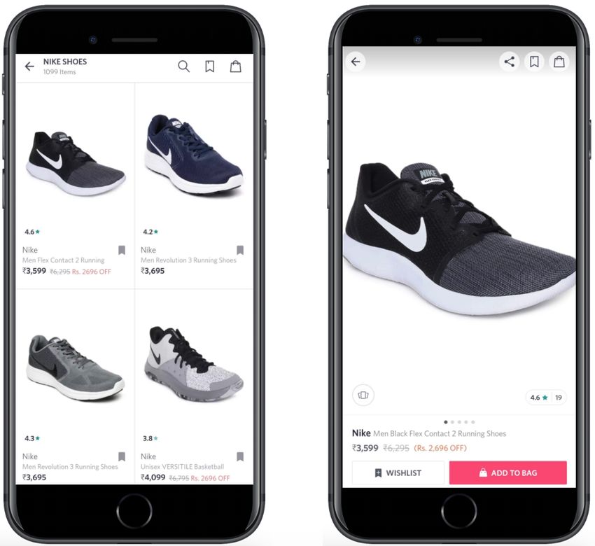
conversion driving factor. As shown in Figure 1, the List Page the products for tomorrow at the base discount value. To get
& product display page (PDP) displays the product(s) with demand at different discount values economics concept of
it's MRP and the discounted price. Product 1,4 is discounted, "Price Elasticity of Demand" (PED) is used. Price elasticity
whereas product 2,3 is selling on MRP. This impacts the click- represents how the demand for a product varies as the price
through rate (CTR) & conversion. Hence, finding an optimal changes. After applying this, we get multiple price-demand
pairs for each product. We have to select a single price point
1 https://www.statista.com/statistics/379046/worldwide-retail-e-
commerce-sales/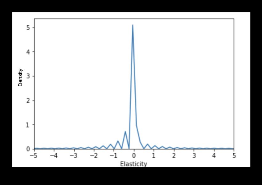
AI4FashionSC KDD, August 23, 2020, Virtual Event, CA, USA                                                             Kedia, et al.

for every product such that the chosen configuration maxi-           Paper [14] describes the price prediction methodology
mizes the overall revenue. To solve it, the Linear Program-      for AWS spot instances. To predict the price for next hour,
ming optimization technique [15] is used. Linear Program-        they've trained a linear model by taking the last three months
ming Problem formulation, along with the constraints, is         & previous 24 hours of historical price points to capture the
described in detail in section 3.4.                              temporal effect. The weights of the linear model is learned
   The solution was deployed in a live production environ-       by applying a Gradient descent based approach. This price
ment, and several A/B Tests were conducted. During the A/B       prediction model works well in this particular case since the
test, A set was shown the same default price, whereas the        number of instances in AWS is very limited. In contrast, in
B set was shown the optimal price suggested by the model.        fashion e-commerce, there can be millions of products, so
As explained in the Result section we're getting a revenue       the methodology mentioned above was not working well in
improvement by approx 1% and gross margin improvement            our case.
by 0.81%.                                                            In paper[13], authors studied how the sales probability of
   The rest of the paper is organized as follows. In Section     the products are affected by customer behaviors and different
2, we briefly discuss the related work. We introduce the         pricing strategies by simulating a Test Market Environment.
Methodology in Section 3 that comprises feature engineering,     They used different learning techniques to estimate the sales
demand prediction model, price elasticity of demand, and         probability from observable market data. In the second step,
linear programming optimization. In Section 4, Results and       they used data-driven dynamic pricing strategies that also
Analysis are discussed, and we conclude the paper in Section     took care of the market competition. They compute the prices
5.                                                               based on the current state as well as taking future states into
                                                                 account. They claim that their approach works even if the
                                                                 number of competitors is significant.
                                                                     Paper [16] authors have explained the optimal price rec-
                                                                 ommendation model for the hosts at the Airbnb platform.
                                                                 Firstly they've applied a binary classification model to pre-
                                                                 dict booking probability of each listing in the platform; after
                                                                 that, a regression model predicts the optimal price for each
                                                                 listing for a night. At last, they apply a personalization layer
                                                                 to generate the final price suggestion to the hosts for their
                                                                 property. This setup is very different from a conventional
                                                                 fashion e-commerce setup where we need to decide an exact
                                                                 price point for all the products, whereas in the former case,
                                                                 it's a range of price.
                                                                     To address the above issues, we've proposed a novel ma-
                                                                 chine learning mechanism to predict the exact price point
                                                                 for all the products on a fashion e-commerce platform at a
                                                                 daily level.

                                                                 3   Methodology
                                                                 In this section, we have explained the methodology of deriv-
              Figure 1. List Page and PDP page                   ing the optimal price point for all the products in the fashion
                                                                 e-commerce platform.
                                                                    Figure 2 shows the architecture diagram to optimize the
2    Related Work
                                                                 price for all the products.
In this section, we've briefly reviewed the current literature
work on Price Optimization in E-commerce. In [7], authors                                      n
                                                                                               Õ
are first creating customer segments using K-means cluster-                               R=         pi q i                    (1)
ing; then, a price range is assigned to each cluster using a                                   i=1
regression model. Post that authors are trying to find out the     Here R is the revenue of the whole platform, pi is the price
customer's likelihood of buying a product using the previous     assigned to i th product, and qi is the quantity sold at that
outcome of user cluster & price range. The customer's like-      price.
lihood is calculated by using the logistic regression model.       According to Equation 1, revenue is highly dependent on
This model gives price range at a user cluster level, whereas    the quantity sold. Quantity sold is, in turn, dependent on
in typical fashion e-commerce exact price point of each prod-    the price of the product. Typically, as the price increases, the
uct is desired.                                                  demand goes down and vice-versa. So there is a trade-off
Price Optimization in Fashion E-commerce AI4FashionSC KDD, August 23, 2020, Virtual Event, CA, USA
The ratio of quantity sold at BAG level (brand, arti-
cle, gender) to the total quantity sold of a product is
calculated to take care of the competitiveness among
substitutable products.
• Sort rank: Search ranking of a product is very highly
correlated with the quantity sold. Products listed in
the top search result generally have higher amounts
sold. The search ranking score has been used for all
the live products to capture this effect in our model.
• Product Embedding: From the clickstream data, the
user-product interaction matrix is generated. The value
Figure 2. Architecture Diagram
of an element in this matrix signifies the implicit score
(click, order count, etc.) of a user's interaction with
between cost and demand. To maximize revenue, we need the product. Skip-gram based model[8] is applied to
demand for all the products at a given price. Therefore, a the interaction matrix, which captures the hidden at-
demand prediction model is required. Predicting demand for tributes of the products in the lower dimension latent
tomorrow at an individual product level is a very challenging space. Word2Vec [12] is used for the implementation
task. For new products, there is a cold start problem which we purpose.
address by using product embeddings. Another challenging
task is how to capture the cannibalization of product. 3.2 Demand Prediction Model
Demand for a product is a continuous variable, hence regres-
3.1 Feature Engineering sion based models, sequence model LSTM, and time series
To estimate the demand for all products in the platform ex- model ARIMA were used to predict future demand for all
tensive feature engineering is done. The features are broadly the products. Since the data obeyed most of the assumptions
categorized into four categories : of linear regression (the linear relationship between input
and output variables, feature independence, each feature
following normal distribution and homoscedasticity), linear
regression became an optimal choice. Hyperparameters like
learning rate (alpha) and max no. of iterations were tuned
using GridSearchCV and by applying 5 fold cross-validation.
The learning rate of 0.01 and the max iteration of 1000 was
chosen as a result of it. Overfitting was taken care of by
using a combination of L1 and L2 regularization (Elastic Net
Regularization). Tree-based models were also used. They
do not need to establish a functional relationship between
input features and output labels, so they are useful when it
comes to demand prediction. Also, trees are much better to
interpret and can be used to explain the outcome to business
users adequately. Various types of tree-based models like
Random Forest and XGBoost were used. Hyperparameters
like depth of the tree and the number of trees were tuned
Figure 3. Feature Engineering for Demand Prediction
using the technique mentioned above. Overfitting was taken
care of by post-pruning the trees. Lastly, a MLP regressor
• Observed features: These features showcase the brows- with a single hidden layer of 100 neurons, relu activation,
ing behavior of people. They include quantity sold, list and Adam optimizer was used. Finally, an ensemble of all
count, product display count, cart count, total inven- the regressors was adopted. The median of the output of
tory, etc. From these features, the model can learn all the regressors was chosen as the final prediction. It was
about the visibility aspects of the products. These di- chosen because each of the individual regressors was not
rectly correlate with the demand for the product. able to learn all aspects of the nature of the demand for the
• Engineered features: To capture the historical trend product and wasn't giving adequate results. Thus, the ensem-
of the products, we've handcrafted multiple features. ble approach was able to capture all aspects of the data and
For example, the last seven days of sales, previous 7 delivered positive results. LSTM with a hidden layer was also
days visibility, etc. They also capture the seasonality used to capture the temporal effects of the sale. Batch-size for
effects and its correlation to the demand of the product. each epoch was chosen in such a way that it comprised of allAI4FashionSC KDD, August 23, 2020, Virtual Event, CA, USA Kedia, et al.
the items of a particular day. Hyperparameters like loss func- A product is said to be highly elastic if for a small change
tion, number of neurons, type of optimization algorithm, and in price there is a huge change in demand, unitary elastic
the number of epochs were tuned by observing the training if the change in price is directly proportional to change in
and validation loss convergence. Mean-squared error loss, demand and is called inelastic if there is a significant change
50 neurons, Adam optimizer, and 1000 epochs were used to in price but not much change in demand.
perform the task. Arima was also used to capture the trends Since we are operating in a fashion e-commerce envi-
and seasonality of the demand for the product. The three ronment determination of price elasticity of demand is a
parameters of ARIMA : p (number of lags of quantity sold to challenging task. There is a wide range of products that are
be used as predictors), q (lagged forecast errors), and d (min- sold, so we experience all types of elasticity. Usually price
imum amount of difference to make series stationery) were and demand share an inverse relationship i.e., when the price
set using the ACF and PACF plots. The order of difference (d) decreases, the demand for that product increases and vice-
= 2 was chosen by observing when the ACF plot approaches versa.
0. The number of lags (p) = 1 was selected by observing the But this relationship is not followed in the case of Gif-
PACF plot and when it exceeds the PACF's plot significance fen/Veblen goods. Giffen/Veblen goods are a type of product,
limit. Lagged forecast errors (q) = 1 was chosen the same for which the demand increases when there is an increase
way as p was chosen but by looking at the ACF plot instead in the price. In our environment, we not only experience
of PACF. different types of elasticity, but we also have to deal with Gif-
fen/Veblen goods. E.g., Rolex watch is a type of Veblen good
3.3 Price Elasticity of Demand as its demand increases with an increase in price because it
From the demand model, we get the demand for a particular is used more as a status symbol.
product for the next day based on its base discount. To get Due to these reasons calculating the price elasticity of
the demand for a product at a different price point, we use demand at a brand, category, or any other global level is not
the concept of price elasticity of demand [1][10]. possible. So we have computed it for each product based on
the historical price-demand pairs for that product. For new
products, the elasticity of similar products determined by
product embeddings were used.
Price elasticity is used to calculate the product demand at
different price points. From the business side, there is a strict
guardrail of max ±δ % change in the base discount, where δ
is a user defined threshold. The value of δ is kept as a small
positive integer since a drastic change in the discounts of the
products is not desired. We have the demand value for all
the products for tomorrow at the base discount by using the
aforementioned demand prediction model. We also calculate
two more demand values by increasing the base discount by
δ % and decreasing by δ % by using the price elasticity. Thus
the output after applying the elasticity concept is that we get
three different price points and the corresponding demand
value for all products. The price elasticity changes with time,
Figure 4. Variation of Price and Demand of a Product
so its value is updated daily.
Figure 4 illustrates the effects of change in price on the 3.4 Linear Programming
quantity demanded of a product. When the price drops from After applying the price elasticity of demand, we get three
INR 1400 to 1200, the quantity demanded of the product different price points for a product and the corresponding
increases from 7 to 11. The price elasticity of demand is used demand at those price points.
to capture this phenomenon. Now we need to choose one of these three prices such that
The formula for price elasticity of demand is : the net revenue is maximized. Given 3 different price points
and N products, there will be 3N permutations in total. Thus,
∆Q P
Ed = . (2) the problem boils down to an optimization problem, and we
Q ∆P
formulate the following integer problem formulation: [5].
where Q, P are the original demand and price for the
product, respectively. ∆Q represents the change in demand as 3 Õ
n
the price changes, and ∆P depicts the change in the product’s
Õ
max pik x ik dik
price. k=1 i=1Price Optimization in Fashion E-commerce AI4FashionSC KDD, August 23, 2020, Virtual Event, CA, USA
Figure 5. Linear Programming Vector Computations
chosen as the optimal price point. The linear programming
Subject To the constraints problem [4] thus obtained is :
3
Õ 3 Õ
n
x ik = 1 ∀ i ∈ n
Õ
max pik x ik dik
k =1 k=1 i=1
3 Õ
Õ n
pik x ik = c Subject To the constraints
k =1 i=1
3
Õ
x ik ∈ {0, 1} x ik = 1 ∀ i ∈ n
k=1
3 Õ
n
In the above equations pik denotes the price and dik denotes Õ
pik x ik = c
the demand for i t h product if k t h price-demand pair is chosen.
k =1 i=1
Here, x ik acts like a mask that is used to select a particular
price for a product. x ik is a boolean variable (0 or 1) where 1 0 ≤ x ik ≤ 1
denotes that we select the price and 0 that we do not select it.
The constraint k3 =1 x ik = 1 makes sure that we select only 1
Í
price for a product and k3 =1 ni=1 pik x ik = c makes sure that
Í Í
We implement the above linear programming problem
sum of all the selected prices is equal to c, where c is user- using Scipy linear programming library routine linprog. The
defined variable. C can be varied from its minimum value that input is given in the vector form as follows:
is obtained when the least price for each product is chosen to
its maximum value that is obtained when the highest price max r.x
for each product is chosen. Somewhere in between, we get Subject To A.x = b
the optimal solution. Where r is a vector that contains the revenue contributed
The above formulation is computationally intractable since by a product at each price point, A is a matrix that contains
there can be millions of permutations of price-demand pairs. information about the products and their prices.
Thus we convert the above integer programming problem As shown in Figure 5, a set of 3 columns represents a
to a linear programming problem by treating x ik as a con- product. In this set of 3 columns, the first column represents
tinuous variable. This technique is called linear relaxation. value corresponding to (discount-δ %), middle column to base
The solution obtained from this problem acts like a linear discount, last column to (discount+δ %). The last row of A
bound for the integer formulation problem. Here, for the i th contains different price points according to their updated
product the price corresponding to maximum value of x ik is discount value & product. b vector contains the upper boundAI4FashionSC KDD, August 23, 2020, Virtual Event, CA, USA Kedia, et al.
of the constraints. All entries in b are 1 except the last one, hence elasticity is calculated at a product level. It is evident
which is equal to c. Here 1 represents that only one price can from the figure that the range of elasticity is from -5 to +5. -5
be selected for each product, and c indicates the summation indicates that if the price is dropped, then demand increases
corresponding to the chosen prices. drastically, and +5 suggests that if the price is increased, then
demand also increases by a large margin. It can be observed
4 Results & Analysis that most of the time, elasticity value is 0; this is so because
In this section, we have discussed the data sources used to 80% of the quantity of the product sold is 0. Lastly, it can be
collect the data, followed by an analysis of the data and the concluded that most of the product’s elasticity lies between
insights derived from it. Different kinds of evaluation metrics -1 to +1. Hence, most of the products are relatively inelastic,
used to check the accuracy are also discussed along with the but there are few products whose elasticity is very high and
comparative study of different models used. are at extreme ends, so it has to be calculated accurately.
4.1 Data Sources
Data was collected from the following sources :
• Clickstream data: this contained all user activity
such as clicks, carts, orders, etc.
• Product Catalog: this contained details of a product
like brand, color, price, and other attributes related to
the product.
• Price data: this contained the price and the quantity
sold of a product at hour level granularity.
• Sort Rank: this contained search rank and the corre-
sponding scores for all the live products on the plat-
form.
4.2 Analysis of Data
According to the analysis, 20% of the products generate 80%
Figure 7. Distribution of Elasticity
of the revenue. Hence, it is required to price these products
precisely. This is the biggest challenge when it comes to de-
mand prediction. Figure 6 shows the distribution of quantity 4.3 Evaluation Metric
To evaluate the demand prediction models, mean absolute
error & root mean squared error is used as a metric. They
both tell us the idea of how much the predicted output is
deviating from the actual label. For this scenario, coefficient
of determination i.e., R 2 or adjusted R 2 , is not a good measure
as it involves the mean of the actual label. Since 80% of the
time actual label is 0 mean cannot accommodate it, and hence
R 2 cannot judge the demand model's performance.
4.4 Results
In this section results of different models are discussed in ta-
ble 1. Majorly three different classes of the model were tested
and compared. They include regressors, LSTM, and ARIMA.
mae and rmse were chosen as the evaluation metric to com-
Figure 6. Distribution of Quantity Sold pare these models. The reason for this choice is discussed in
section 4.3. All the models were trained on historical data of
sold for all the products on the platform. It is evident that a the past three months, comprising of over a million records.
minority of products contribute towards the total revenue. For the test data, the recent single day records were used.
Figure 7 shows the elasticity distribution of the products First, different kinds of regressors were used; out of all the
on the platform. The y-axis of the graph depicts the density regressors, XGBoost gave the best result. It is so because it’s
rather than the actual count frequency of the elasticity value. tough to establish a functional relationship between input
As discussed in Section 3.3, the determination of elasticity is features and output demand. As XGBoost does not need to
a difficult task. All kinds of elasticity are experienced, and establish any functional relationship, it performed better.Price Optimization in Fashion E-commerce AI4FashionSC KDD, August 23, 2020, Virtual Event, CA, USA
Model mae rmse Percentage increment in Revenue GM % Uplift
Linear Regression 0.207 0.732 Test 1 0.96% 0.99%
Random Forest Regressor 0.219 0.854 Test 2 1.96% 0.95%
XG Boost 0.195 0.847 Test 3 0.09% 0.49%
MLP Regressor 0.254 1.471 Test 4 3.27% -0.41%
Ensemble 0.192 0.774 Test 5 7.05% 0.15%
LSTM 0.221 0.912 Table 2. A/B test results
ARIMA 0.258 1.497
Table 1. Comparative performance of various models
In the case of Women's Western wear, there was a massive
lift in revenue, but the gross margin fell. The reason for this
However, all individual regressors were not able to capture is that women's products were highly elastic. Small changes
all aspects of the data, so an ensemble of all the regressors in price had a significant impact on demand. So due to the
gave the ideal result. The ensemble takes advantage of all model’s recommended price, there was a vast fluctuation in
regressors and hence is chosen. Then, after regressors, LSTM demand (i.e., demand for products increased), and the rev-
& ARIMA were also tried, but it failed to give the desired enue thus increased. However, the gross margin was slightly
result as due to multiple external factors in the business, the impacted, and it decreased.
demand data for the products did not exhibit sequential & Eyewear is a small business unit, so the impact of discount
temporal characteristics. change is enormous, i.e., 7.05% increment in the revenue,
whereas the GM increased by 0.15%.
4.5 Experimental Design
Overall there was an approximately 1% increase in revenue
In this section, we describe live experiments that were per- of the platform and 0.81% uplift in gross margin due to model
formed on one of the largest fashion e-commerce platforms. recommended prices. These are computed by taking the
The experiments were run on around two hundred thousand average of the first three instances since they belong to the
styles spread across five days. To test the hypothesis that same business unit.
model recommended prices are better than baseline prices,
two user groups were created: 5 Conclusion
Fashion e-tailers currently find it extremely hard to decide
• Set-A (Control group) was shown the baseline prices an optimal price & discounting for all the products on a daily
• Set-B (Treatment group) was shown model recom- basis, which can maximize the overall net revenue & the
mended prices. profitability. To solve this, we have proposed a novel method
comprising three major components. First, a demand predic-
These sets were created using a random assignment from tion model is used to get an accurate estimate of tomorrow's
the set of live users. 50% of the total live users were assigned demand. Then, the concept of price elasticity of demand is
to Set A and the rest to Set B. used to get the demand for a product at multiple price points.
Users in Control and Treatment groups were exposed to Finally, a linear programming optimization technique is used
the same product. But the products were priced differently to select one price point for each product, which maximizes
according to the group they belong to. Both groups were the overall revenue. Online A/B test experiments show that
compared with respect to the overall platform revenue and by deploying the model revenue and gross margin increases.
gross margin. Revenue is already defined and explained in Right now, the prices are decided and updated daily, but in
section 3, whereas gross margin can be defined as follows : the future, we would like to extend our work so that we can
also capture the intra-day signals in our model & accordingly
GrossMarдin = (Revenue − (buyinд cost))/Revenue do the intra-day dynamic pricing.
In general, the gross margin in our scenario is pure profit References
bottom line. [1] M Babar, PH Nguyen, V Cuk, and IG Kamphuis. 2015. The development
In table 2, the first three instances correspond to the busi- of demand elasticity model for demand response in the retail market
ness unit - Men's Jeans and Streetwear, while the last 2 are environment. In 2015 IEEE Eindhoven PowerTech. IEEE, 1–6.
of Women's Western wear and Eyewear respectively. [2] Tianqi Chen and Carlos Guestrin. 2016. Xgboost: A scalable tree
In the case of Men's Jeans and Streetwear, there is a steady boosting system. In Proceedings of the 22nd acm sigkdd international
conference on knowledge discovery and data mining. ACM, 785–794.
increase in both revenue and gross margin of the whole [3] Javier Contreras, Rosario Espinola, Francisco J Nogales, and Antonio J
platform. From this, it can be concluded that the model rec- Conejo. 2003. ARIMA models to predict next-day electricity prices.
ommended price gave positive results for this business unit. IEEE transactions on power systems 18, 3 (2003), 1014–1020.AI4FashionSC KDD, August 23, 2020, Virtual Event, CA, USA Kedia, et al.
[4] MAH Dempster and JP Hutton. 1999. Pricing American stock options Cat. No. 03EX693), Vol. 2. IEEE, 893–898.
by linear programming. Mathematical Finance 9, 3 (1999), 229–254. [11] Xueheng Qiu, Le Zhang, Ye Ren, Ponnuthurai N Suganthan, and Gehan
[5] Ralph E Gomory and William J Baumol. 1960. Integer programming Amaratunga. 2014. Ensemble deep learning for regression and time se-
and pricing. Econometrica: Journal of the Econometric Society (1960), ries forecasting. In 2014 IEEE symposium on computational intelligence
521–550. in ensemble learning (CIEL). IEEE, 1–6.
[6] Klaus Greff, Rupesh K Srivastava, Jan Koutník, Bas R Steunebrink, [12] Xin Rong. 2014. word2vec parameter learning explained. arXiv preprint
and Jürgen Schmidhuber. 2016. LSTM: A search space odyssey. IEEE arXiv:1411.2738 (2014).
transactions on neural networks and learning systems 28, 10 (2016), [13] Rainer Schlosser and Martin Boissier. 2018. Dynamic pricing under
2222–2232. competition on online marketplaces: A data-driven approach. In Pro-
[7] Rajan Gupta and Chaitanya Pathak. 2014. A Machine Learning Frame- ceedings of the 24th ACM SIGKDD International Conference on Knowl-
work for Predicting Purchase by Online Customers based on Dynamic edge Discovery & Data Mining. ACM, 705–714.
Pricing. In Complex Adaptive Systems. [14] Vivek Kumar Singh and Kaushik Dutta. 2015. Dynamic Price Prediction
[8] David Guthrie, Ben Allison, Wei Liu, Louise Guthrie, and Yorick Wilks. for Amazon Spot Instances. 2015 48th Hawaii International Conference
2006. A closer look at skip-gram modelling.. In LREC. 1222–1225. on System Sciences (2015), 1513–1520.
[9] Maobin Li, Shouwen Ji, and Gang Liu. 2018. Forecasting of Chinese [15] Daniel Solow. 2007. Linear and nonlinear programming. Wiley Ency-
E-Commerce Sales: An Empirical Comparison of ARIMA, Nonlinear clopedia of Computer Science and Engineering (2007).
Autoregressive Neural Network, and a Combined ARIMA-NARNN [16] Peng Ye, Julian Qian, Jieying Chen, Chen-hung Wu, Yitong Zhou,
Model. Mathematical Problems in Engineering 2018 (2018). Spencer De Mars, Frank Yang, and Li Zhang. 2018. Customized Re-
[10] Lusajo M Minga, Yu-Qiang Feng, and Yi-Jun Li. 2003. Dynamic pricing: gression Model for Airbnb Dynamic Pricing. In Proceedings of the 24th
ecommerce-oriented price setting algorithm. In Proceedings of the 2003 ACM SIGKDD International Conference on Knowledge Discovery & Data
International Conference on Machine Learning and Cybernetics (IEEE Mining. ACM, 932–940.You can also read