A comparative study on image based snake identification using machine learning
←
→
Page content transcription
If your browser does not render page correctly, please read the page content below
www.nature.com/scientificreports
OPEN A comparative study
on image‑based snake
identification using machine
learning
Mahdi Rajabizadeh & Mansoor Rezghi*
Automated snake image identification is important from different points of view, most importantly,
snake bite management. Auto-identification of snake images might help the avoidance of venomous
snakes and also providing better treatment for patients. In this study, for the first time, it’s been
attempted to compare the accuracy of a series of state-of-the-art machine learning methods, ranging
from the holistic to neural network algorithms. The study is performed on six snake species in Lar
National Park, Tehran Province, Iran. In this research, the holistic methods [k-nearest neighbors
(kNN), support vector machine (SVM) and logistic regression (LR)] are used in combination with
a dimension reduction approach [principle component analysis (PCA) and linear discriminant
analysis (LDA)] as the feature extractor. In holistic methods (kNN, SVM, LR), the classifier in
combination with PCA does not yield an accuracy of more than 50%, But the use of LDA to extract
the important features significantly improves the performance of the classifier. A combination of
LDA and SVM (kernel = ’rbf’) is achieved to a test accuracy of 84%. Compared to holistic methods,
convolutional neural networks show similar to better performance, and accuracy reaches 93.16%
using MobileNetV2. Visualizing intermediate activation layers in VGG model reveals that just in deep
activation layers, the color pattern and the shape of the snake contribute to the discrimination of
snake species. This study presents MobileNetV2 as a powerful deep convolutional neural network
algorithm for snake image classification that could be used even on mobile devices. This finding pave
the road for generating mobile applications for snake image identification.
With around 81.410 to 137.880 deaths per year (https://w ww.w ho.i nt), snakes are among the top three dangerous
animals for human. Out of 3848 known species of snakes, around 800 species are venomous, among which only
about 50 species are fatal to human (https://www.reptile-database.reptarium.cz).
Identification of snakes is not easy; For example, those characters discriminating the non-venomous snake
from the viperids (oval shaped head, round pupil, absence of a pit) occur in the elapid snakes either; while
both viperids and elapids are venomous or fatal to the human. Hence, proper snake identification would entail
herpetological skills that use body and head morphological features (color, pattern, shape, scalation, and etc.)1.
Automated snake image identification is important from different points of view, most importantly, snake bite
management. Auto-identification of snake images might help people avoid venomous snakes; besides, it can help
healthcare providers plan a better treatment for patients bitten by snakes (see2).
Computer vision technology has developed rapidly in the field of automated image recognition and image
classification3. Computer scientists apply different machine learning approaches for image c lassification4. Image
classification using machine learning, consists of two phases: feature extraction and classification. In image clas-
sification the classes are predetermined; in summary, the process includes a training phase using the training
data, and classification of the test data based on the trained model. By training, the predefined classes can be
conceived of an available dataset that take the characteristic features of each image classes and shape a special
description for each specific c lass5.
Application of machine learning (hereafter ML) for the identification of plants and animals’ images is growing
rapidly (for a review see6). Recently, efforts have been made for image-based snake classification using ML7–10.
In these researches a range of machine learning methods we used, from traditional ML classifiers, including
k-nearest neighbors (hereafter kNN) and support vector machine (hereafter SVM), to the state of the art neural
Department of Computer Science, Tarbiat Modares University, Tehran, Iran. *email: rezghi@modares.ac.ir
Scientific Reports | (2021) 11:19142 | https://doi.org/10.1038/s41598-021-96031-1 1
Vol.:(0123456789)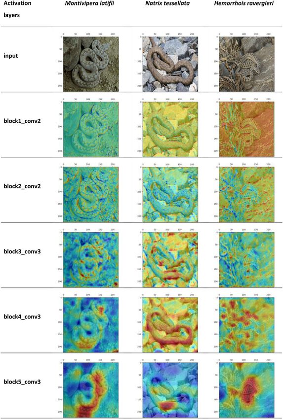
www.nature.com/scientificreports/
Figure 1. Scatterplot resulting from PCA over snake images.
network algorithms like convolutional neural network (hereafter CNN). None of the former studies compared
the accuracy of the traditional methods and neural networks in the classification of the snake images; neverthe-
less, there are challenges in the application of ML algorithms for the classification of snakes.
• First, because of the elongated and flexible body, snakes usually represent wide variations in the pose and
deformation of the body. For example, in a limited image dataset of a snake, head or tail might be hidden
under the body; besides, the body itself might be twisted in different directions and hence, the dorsal color
pattern might show plenty of different ornamentations. So, acquiring features from the dorsal body pattern
of snakes is quite challenging.
• Second, training a deep convolutional neural network requires a large image dataset. Unfortunately, not
many specialized datasets are available for snakes. Regarding rare snakes this situation is even worse; On
the other hand, since the museum specimens do not have natural color and pose, they are not applicable for
incorporation in the whole body image datasets.
In this study, for the first time, it’s been planned to compare the accuracy of a series of state-of-the-art machine
learning methods, ranging from the traditional to neural network algorithms. An attempt is made to evaluate the
performance of these models in the classification of a limited, accessible series of snake images. For this purpose,
the following guidelines are pursued:
• Minimum possible dataset: collecting snake images is not an easy task, and not all the images are necessarily
taxonomically informative (e.g. art works). So, a dataset of 594 images of the whole body of six snake spe-
cies were collected. Only those images in which at least 50% of the snake body was visible in the image were
involved in the dataset.
• Feature extraction: to overcome the challenge of wide variations in the body pose of snakes in the images,
a feature extraction method has been used in combination with traditional classifiers. Feature extraction
is the process of representing a raw image in its reduced form to facilitate decision-making as to pattern
classification11.
• Transfer learning: the size of our dataset is not optimum to train a state-of-the-art deep neural network
model; To solve this issue, a transfer learning is used. In this method, off-the-shelf features extracted from a
pre-trained network is transferred to a new CNN model12 for classification of snakes.
• Visualization of CNN hidden layers: to understand the learning process of a CNN model, a visualization
method has been used, which visualizes the location of the discriminative regions of snakes’ images at each
hidden layer13. Using this method, we can uncover snake identification process through a CNN model and
also compare it with human experts.
Results
Principle component analysis (PCA). PCA extracted 476 components. The first three components
cumulatively explain 23.39, 25.83 and 26.78% of the total variance (Fig. 1).
Linear discriminant analysis (LDA). LDA extracted five components; all of which cumulatively explain
28.22, 49.98, 70.49, 86.16 and 100% of total variance (Fig. 2).
kNN classifier. The accuracy of kNN algorithm used for the classification of snake images, merely and in
combination with a data dimension reduction approach, is presented in Figs. 3 and 4; while k in these procedures
has been changing in a range from 1 to 30.
Scientific Reports | (2021) 11:19142 | https://doi.org/10.1038/s41598-021-96031-1 2
Vol:.(1234567890)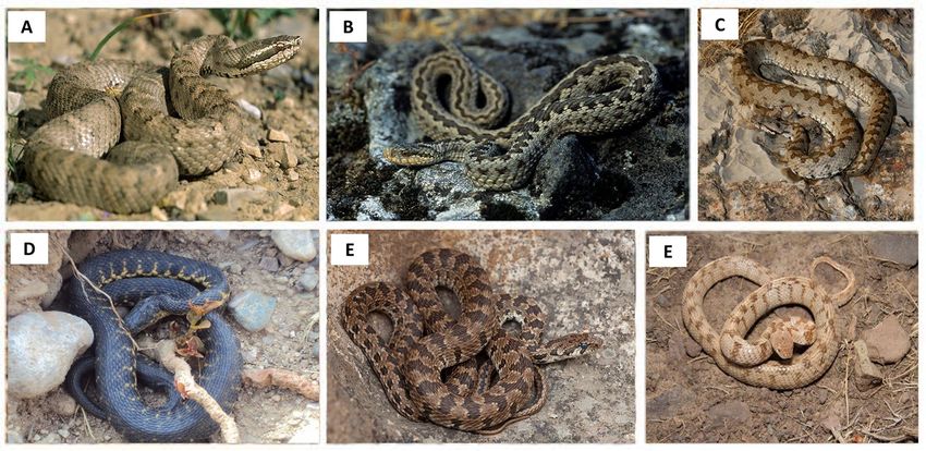
www.nature.com/scientificreports/

                                  Figure 2.  Scatterplot resulting from linear discriminant analysis (LDA) over the snake images.

                                  Figure 3.  Results of snake image classification using kNN algorithm, as well as kNN in combination with a data
                                  dimension reduction approach (PCA), while k has been changing in a range from 1 to 30. The number of the
                                  components (c) is 5, 10, 50, 100 and 200.

                                  SVM. The result of snake image classification using SVM algorithm, both alone and in combination with a
                                  data dimension reduction approach, is presented in Table 1.

                                  Logistic regression. The result of snake image classification using logistic regression algorithm, both alone
                                  and in combination with a data dimension reduction approach, is presented in Table 2.

                                  CNN.      The VGG-16 model involves 134.260.544 parameters. The model was trained for 500 epochs. Besides,
                                  the MobileNetV2 involves 5.147.206 parameters and was trained for 150 epochs. Both the models were set up
                                  with SGD optimizer and a learning rate equal to 0.0001, as well as a momentum equal to 0.9 (Table 3).
                                     The models were run twice; once without an initial weight and another time with an initial weight from
                                  ImageNet. The models without the initial weight were not trained properly during the training process. In
                                  VGG-16, the train and test accuracy of the weighted model after one run reached to 96.82 and 77.78%; while in
                                  MobileNetV2 the train and test accuracy of the weighted model reached to above 90%. Hence a fivefold valida-
                                  tion set were performed for MobileNetV2 and the accuracy obtained for the train and test of the model were
                                  99.16 and 89.99%, 99.16 and 93.33%, 99.78 and 93.33%, 99.58 and 92.50%, and finally 100.0 and 91.67% (Fig. 5).
                                  MobileNetV2 model is a relatively robust model and induced noise in the input test images does not reduce the
                                  accuracy of the model drastically (Table 4). The Detailed result of snake image classification, using VGG-16 and

Scientific Reports |   (2021) 11:19142 |              https://doi.org/10.1038/s41598-021-96031-1                                                3

                                                                                                                                           Vol.:(0123456789)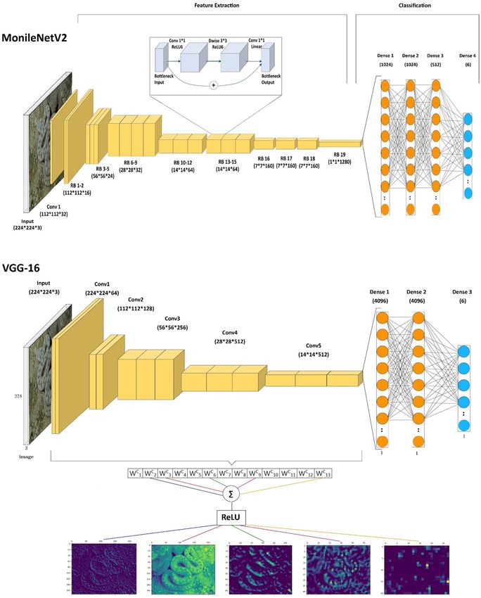
www.nature.com/scientificreports/

                                            Figure 4.  Result of snake image classification using kNN algorithm, as well as kNN in combination with a
                                            data dimension reduction approach (LDA), while k has been changing in a range from 1 to 30. The number of
                                            components (comp) was ranging from 2 to 5.

                                                                                                                                         SVM_PCA (Nr. components: 2, 5, 10, 20, 50, 100,
                                                                            SVM_LDA (Nr. components: 2, 3, 4, 5)                         200)                                                       SVM
                                             Classifier (SVM)               Tr                            Ts                             Tr                           Ts                            Tr       Ts
                                             kernel = ’linear’              0.68, 0.77, 0.83, 0.83        0.66, 0.76, 0.81,0.81          –,–,–,–,–, 1, 1              –,–,–,–,–, 0.31, 0.30         1.00     0.40
                                                                                                                                         0.31, 0.45, 0.49, 0.52, 0.44, 0.27, 0.34, 0.36, 0.33, 0.31,
                                             kernel = ’poly’, dr = 5        0.55, 0.63, 0.72, 0.72        0.52, 0.60, 0.68, 0.64                                                                     1.00    0.34
                                                                                                                                         0.55, 0.60                    0.29, 0.27
                                                                                                                                         0.36, 0.50, 0.57, 0.65, 0.73, 0.31, 0.41, 0.42, 0.41, 0.45,
                                             kernel = ’rbf ’                0.71, 0.79, 0.87, 0.87        0.69, 0.76, 0.83, 0.84                                                                     0.93    0.43
                                                                                                                                         0.79, 0.83                    0.44, 0.43
                                                                                                                                         0.16, 0.20, 0.21, 0.23, 0.28, 0.14, 0.18, 0.20, 0.21, 0.22,
                                             kernel = ’sigmoid’             0.52, 0.63, 0.77, 0.79        0.50, 0.61, 0.76, 0.79                                                                     0.20    0.20
                                                                                                                                         0.34, 0.43                    0.23, 0.26

                                            Table 1.  Result of snake image classification using SVM algorithm.

                                                                                                                                                              LR_LDA (Nr. components: 2,
                                                               LR_PCA (Nr. components: 2, 5, 10, 20, 50, 100, 200)                                            3, 4, 5)                              LR
                                                               Tr                                                  Ts                                         Tr                 Ts                 Tr      Ts
                                             tol = 1e−2        0.25, 0.31, 0.36, 0.43, 0.57, 0.88, 1.0             0.23, 0.30, 0.30, 0.33, 0.32, 0.31, 0.35   –, –, 0.77, 0.84   –, –, 0.76, 0.83   1.0     0.35
                                             tol = 1e−3        0.25, 0.28, 0.33, 0.41,0.56, 0.88, 1, 0             0.24, 0.27, 0.27, 0.30, 0.30, 0.30, 0.32   –, –, 0.77, 0.85   –, –, 0.78, 0.84   1.0     0.37
                                             tol = 1e−4        0.25, 0.27, 0.33, 0.40, 0.56, 0.85, 1.0             0.23, 0.24, 0.26, 0.28, 0.31, 0.27, 0.34   –, –, 0.78, 0.82   –, –, 0.77, 0.81   1.0     0.36

                                            Table 2.  Result of snake image classification using logistic regression algorithm.

                                                                 MobileNetV2                                   VGG-16
                                                                 G      H        M    N     V        T         G        H     M     N      V     T
                                             Gloydius            22     0        1    2     0        0         20       2    1      1      0     1
                                             Hemorrhois          1      16       0    0     0        1         1        16   0      0      0     1
                                             Montivipera         0      0        24   1     0        0         0        1    21     1      0     2
                                             Natrix              0      1        0    18    0        0         2        2    2      9      0     4
                                             Viper               0      0        0    1     13       0         1        1    0      0      12    0
                                             Telescopus          0      0        0    0     0        16        1        0    1      1      0     13
                                             Total               25    18        25   19    14       16        25       18   25     19     14    16

                                            Table 3.  Confusion matrix showing the performance of MobileNetV2 and VGG-16 model for snake image
                                            classification of the test dataset. Total number of the samples has been presented bellow each column.

          Scientific Reports |   (2021) 11:19142 |                           https://doi.org/10.1038/s41598-021-96031-1                                                                                             4

Vol:.(1234567890)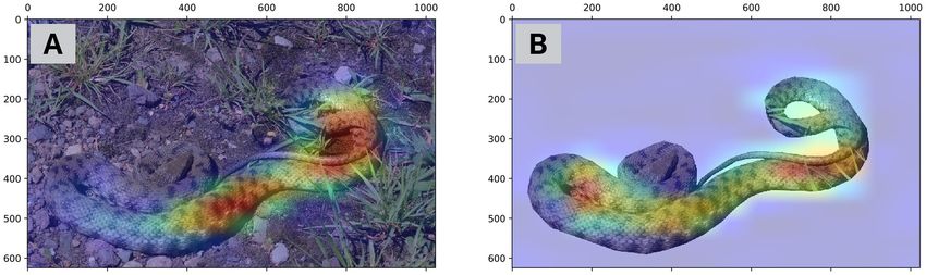
www.nature.com/scientificreports/

                                              1

                                             0.9

                                             0.8

                                             0.7

                                             0.6

                                  Accuracy   0.5

                                             0.4

                                             0.3                                                                        MobileNetV2

                                             0.2
                                                                                                                        VGG-16
                                             0.1

                                              0
                                                   0   100            200            300            400           500
                                                                            Epoch
                                              2

                                             1.8

                                             1.6

                                             1.4

                                             1.2
                                  Loss

                                              1

                                             0.8
                                                                                                                        MobileNetV2
                                             0.6

                                             0.4                                                                        VGG-16

                                             0.2

                                              0
                                                   0   100            200           300             400          500
                                                                            Epoch
                                  Figure 5.  Accuracy and loss values of MobileNetV2 and VGG-16 model with an initial weight from ImageNet
                                  during the training process.

                                  MobileNetV2 algorithm, has been presented in a confusion matrix (Table 3); moreover an accuracy results table
                                  has been presented in Table 5.
                                      Visualizing the intermediate activation layers in VGG-16 (and similarly MobileNetV2) model revealed that
                                  although a snake and its environmental features are considered together via the model’s filters in the first and
                                  second blocks of the activation layers toward the deeper layers, the model focuses on the dorsal pattern features
                                  of the snakes as the discriminant feature (Fig. 6).

Scientific Reports |   (2021) 11:19142 |               https://doi.org/10.1038/s41598-021-96031-1                                                5

                                                                                                                                            Vol.:(0123456789)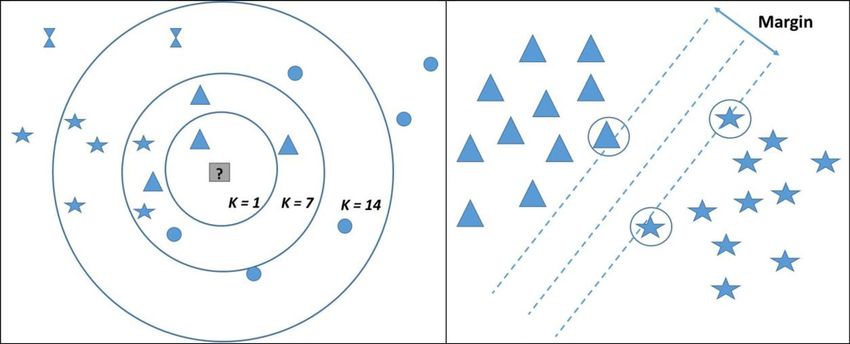
www.nature.com/scientificreports/
Width shifted Flipped and zoomed
F1-score F1-score
Gloydius 0.89 0.84
Hemorrhois 0.89 0.73
Montivipera 0.9 0.85
Natrix 0.87 0.75
Vipera 0.96 0.83
Telescopus 0.94 0.89
Accuracy 0.91 0.82
Table 4. The F1-score and overall accuracy of MobileNetV2 model for modified test images datasets
(augmented via width shift as well as vertical flip and zooming) showing the robustness of the model.
MobileNetV2 VGG-16
Precision Recall F1-score Precision Recall F1-score
Gloydius 0.96 0.88 0.92 0.8 0.8 0.8
Hemorrhois 0.89 0.89 0.89 0.73 0.89 0.8
Montivipera 0.96 0.92 0.94 0.84 0.84 0.84
Natrix 0.82 0.95 0.88 0.75 0.47 0.58
Vipera 1 0.93 0.96 1 0.86 0.92
Telescopus 0.94 1 0.97 0.62 0.81 0.7
Accuracy 0.93 0.78
Table 5. Accuracy result of MobileNetV2 and VGG-16 model for snake image classification.
Discussion
In this study, for the first time, a series of state-of-the-art machine learning algorithms were compared in the
classification of six snake species of Lar National Park. In holistic methods (kNN, SVM, LR), performance of the
classifiers over the raw images’ data were not satisfying and the test accuracy did not exceed 50%. Application
of the dimension reduction algorithms had different outputs; Application of PCA did not improve the accuracy
of the model, but the use of LDA in extracting the important features significantly improved the performance of
classifiers. A combination of LDA and SVM (kernel = ’rbf ’) reached a test accuracy of 84%.
Independent comparative studies of PCA and LDA on the FERET image datasets revealed that a particular
combination of PCA or LDA with a classifier is not always the best combination for classification of each dataset,
so choosing a dimension reduction approach depends on the dataset and the specific t ask14. Amir et al.8 used
Color and Edge Directivity Descriptor (CEDD) as feature extractor. CEDD is a low-level feature that is extracted
from images and might be used for indexing and r etrieval15; Hence, in the classification of snake images of Perlis
corpus dataset (including 349 images of 22 species of the snakes from Perlis Region in Malaysia), they used kNN
(k = 1) and reached the accuracy of 89.22% (correct predictions).
James9 proposed a method that included manually cropping of 31 taxonomic features from snakes’ head and
body images. Snake features are subsequently classified using the proposed method based on kNN algorithm.
He used this method for classification of Elapid and Viperid snakes (two classes) and obtained the accuracy of
94.27%.
Compared to the holistic methods, the performance of neural network algorithms in image classification of
snakes of Lar National Park was not the same. Although the performance of VGG-16 (Table 5) was not different
than the holistic methods, but the image classification accuracy improved drastically using the MobileNetV2
(93.16%). the convolutional neural networks showed better performance than the holistic methods for image-
based fish species’ classification16 and also plant leaf disease17. But opposite results are also reported, e.g. in auto
identification of bird i mages18.
Scientific Reports | (2021) 11:19142 | https://doi.org/10.1038/s41598-021-96031-1 6
Vol:.(1234567890)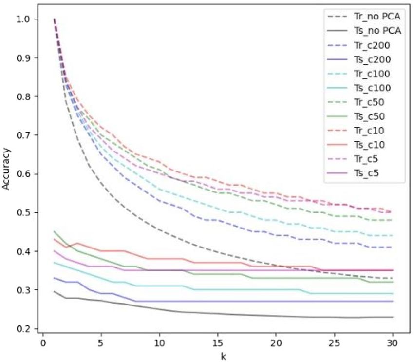
www.nature.com/scientificreports/

                                  Figure 6.  The heatmap visualization of discriminative regions within the hidden activation layers of VGG-16
                                  model.

Scientific Reports |   (2021) 11:19142 |              https://doi.org/10.1038/s41598-021-96031-1                                                 7

                                                                                                                                          Vol.:(0123456789)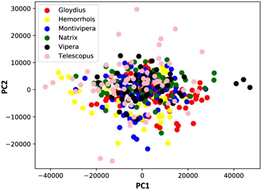
www.nature.com/scientificreports/
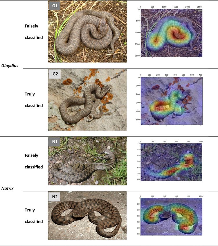
Figure 7. The heatmap visualization of discriminative regions within the last activation layers of VGG-16
model, in truly and falsely classified images of Gloydius and Natrix snakes.
Patel et al.10 used a region-based convolutional neural network (R-CNN) for the detection and classification
of nine snake species in Galápagos Islands and Ecuador; and using ResNet algorithm, they obtained an accuracy
of around 75%, and using VGG-16, they obtained an accuracy of around 70% (Table 6).
So, in this paper we present MobileNetV2, as a powerful deep convolutional neural network algorithm for
snake image classification, with an accuracy over 90%. Since MobileNetV2 is a light algorithm with few number
of parameters, it could be used even on mobile devices. This possibility could be used in a mobile application
that would be helpful e.g. in auto-identification of snake images by healthcare providers to help in snake bite
management. Although the majority of the images used in this study come from SLR cameras, but to feed the
classification model, the images were originally resized to 224*224 pixels that is far bellow the quality of images
of modern smartphone camera. So, smartphone images could be properly used for training a MobileNetV2
model too.
Scientific Reports | (2021) 11:19142 | https://doi.org/10.1038/s41598-021-96031-1 8
Vol:.(1234567890)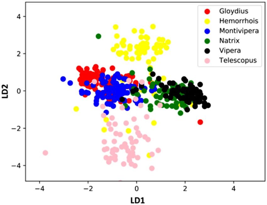
www.nature.com/scientificreports/
Figure 8. The heatmap visualization of the discriminative regions within the last activation layers of VGG-16
model, in Natrix (A: correspond to N1 in Fig. 7) snake, after removing the natural substrates (B).
Visualization of intermediate activation layers in VGG-16 (and similarly MobileNetV2) model reveals that
the model mainly focuses on dorsal color pattern of snakes for a proper classification. Dorsal color pattern is a
taxonomic key feature in the identification of s nakes1. Looking at those snake images that are misidentified, and
comparing them with the similar images that are truly classified (Fig. 7) reveals that in the misclassified images,
the dorsal color pattern has not received a proper attention by the VGG-16 algorithm. This problem might have
raised from the following cases:
• Dorsal pattern is not discriminative enough to identify the snake. For example, in a Gloydius snake (Fig. 7,
G1), dorsal pattern is less pronounced than other specimens of the Gloydius (Fig. 7, G2), probably because
the photographed snake was close to shedding and its dorsal pattern was somehow masked. Similar reason for
misidentification was observe in classification of vector mosquitoes. Park et al.19 observed that if the lighting
condition of the mosquito images are not good enough to clearly show the discriminating color features of
the mosquitoes, the CNN model cannot identify them properly.
• Only a part of the snake’s dorsal pattern has received attention by the model. For example, in Fig. 7 (N1 and
N2), the dorsal patterns are discriminative; whereas in N1 that only part of the pattern has received proper
attention, the image is misidentified. This probably resulted from the cryptic effect of snake over its natural
environment; hence, when the environment is removed from the image (Fig. 8, the overall color pattern of
the snake receives more attention by the model. In classification of Chinese butterfly Xi et al.20 showed that
image background removal enhanced model generalizability and provide a better results for test datasets.
Transfer learning is usually applied when a new dataset smaller than the original dataset is used to train the
pre-trained model. ImageNet is an optimum dataset, but collecting enough number of images from the living
organisms, especially not common ones, like many snake species, is not usually possible. Transfer learning greatly
helps generate high accuracy models for the identification of living creatures. This technique was used success-
osquitoes19 and fish species21,22 too.
fully in generating models for the identification of e.g. vector m
Materials and methods
Study area. The study area is Lar National Park, located in the northeastern Tehran Province, Iran. The park
is a natural attraction, adjacent to Damavand Summit, where many visitors come for picnic, hiking, climbing,
fishing etc.in springs and summer.s As well, nomad families and beekeepers reside in the area during warm sea-
sons. Six snake species have been reported in Lar National Park, including three venomous, one semi-venomous,
and two non-venomous snakes1 (Table 6) .
Dataset. Totally, 594 images of the six snake species of Lar National Park were collected, including 124
images of Caucasian pit viper, 80 of Alburzi viper, 124 of Latifi’s viper, 95 of dice snake, 90 of spotted whip snake,
and 81 of European cat snake (Fig. 9). The images were collected from personal archives (see the acknowl-
edgement) and web databases, including https://www.calphotos.berkeley.edu and https://www.flickr.com. The
images are of different sizes, with 24 bit RGB channels.
Models. A series of state-of-the-art machine learning algorithms were used to compare their performed.
This comparison was performed because in classification of biodiversity elements, depending on the subject,
the performance of different classification algorithms may vary a lot and although for some taxa, deep learning
erformance16,17, for other taxa, shallow learning algorithms work b
algorithms show better p etter18. The methods
are as follows:
Traditional or holistic methods. These methods represent images using the entire image region23. In this
research, the holistic methods were used in combination with a dimension reduction approach. Projecting
images onto a low-dimensional space is used to extract the important features and to discard the redundant
Scientific Reports | (2021) 11:19142 | https://doi.org/10.1038/s41598-021-96031-1 9
Vol.:(0123456789)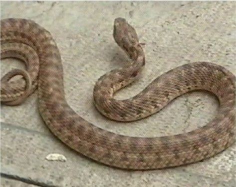
www.nature.com/scientificreports/
Nr English name Scientific name Venom Lethality Human conflict
1 Alburzi viper Vipera eriwanensis Venomous Low (LD50: 21.7) Low
2 Caucasian pit viper Gloydius halys caucasicus Venomous Medium (LD50: 13.6) High
3 Dice snake Natrix tessellate Non-venomous –- High
4 European cat snake Telescopus fallax Semi-venomous Very low Medium
5 Latifi’s viper Montivipera latifii Venomous High (LD50: 5.5) Medium
6 Spotted whip snake Hemorrhois ravergieri Semi-venomous –- High
Table 6. Diversity of snakes of Lar National Park (following1).
Figure 9. Samples of the images of the six snake species of Lar National Park. A: Caucasian pit viper, venomous;
B: Alburzi viper, venomous; C: Latifi’s viper, venomous; D: Dice snake, non-venomous; E: Spotted whip snake,
non-venomous; F: European cat snake, semi-venomous.
details that are not needed for image c lassification23. Feature extraction could be defined as the act of mapping
the image from image space to the feature s pace4. Among the popular approaches in this category, principle
component analysis (PCA) and linear discriminant analysis (LDA) were used.
Principal component analysis. PCA is an unsupervised linear technique that uses an orthogonal transforma-
tion to project a set of variables into a lower dimension with maximum variance. In PCA a set of variables that are
possibly correlated, convert into a set of values that are not correlated variables, called principal components24.
To reduce each data xi ∈ Rn to yi ∈ Rd while d ≪ n, the PCA tries to find orthogonal matrix U ∈ Rn×d so that the
reduced data yi = UTxi have the maximum variance. It has been shown that this projection matrix U ∈ Rn×d con-
sists of d eigenvectors corresponding to the first k large eigenvalues of the following covariance matrix.
1
C= (xi − x)(xi − x)T (1)
N −1
where x and N are mean and the number of data, respectively25.
Linear discriminant analysis. LDA is a supervised feature extraction method that is usually used for the classifi-
cation problems. LDA extracts low dimensional features which have the most sensitive discriminant ability from
high dimensional feature s pace26. LDA for each data xi tries to find an orthogonal projector U by minimizing the
within-class distance and maximizing the between-class distance of the projected data yi = UTxi. Mathematically, If
we consider the number of classes equal to K and consider the number of elements within the class k represented
as Nk, then the index of maximizing the between-class separation and minimizing the within-class separation,
leads to the maximizing the following objective function named Fisher discriminant analysis (FD) as:
trace (U T SB U)
J(W) = (2)
trace (U T SW U)
Scientific Reports | (2021) 11:19142 | https://doi.org/10.1038/s41598-021-96031-1 10
Vol:.(1234567890)www.nature.com/scientificreports/
Figure 10. Left: A simplified, schematic drawing, showing a feature distance space and the classification process
based on the nearest neighbors classifier. Given k = 1, the query image (question mark) is assigned to the label
triangle. Right: A simplified, schematic drawing, showing the process of SVM classification. In multidimensional
feature space, SVM finds the hyperplane that maximizes the margin between the classes (here two classes). Here,
the support vectors are the circled labels.
Here, SW is the within-class distribution and SB is the between-class distribution of the original data, and
they are defined as:
K
SB = Nk (mk − m)(mk − m)T (3)
k=1
K
SW = (xn − mk )(xn − mk )T (4)
k=1 xn ∈Ck
where m and mk are the mean of total data and the mean of the class k. LDA tries to find the matrix U ∈ Rn×d to
maximize Eq. (3). in this regard, each data of x ∈ Rn is linearly transmitted to a d dimension space, as y = UTx .
We can show that the result of maximizing Eq. (3), is d eigenvector, corresponding to the biggest eigenvalue of
the following Generalized eigenvalue problem (Eq. 5)27,28.
SB u = SW u (5)
Traditional or holistic classifiers. Three types of traditional or holistic classifiers have been used in this study
as follows. The training process in these classification algorithms only consist of storing the feature vectors and
labels of the training images.
k‑nearest neighbor. kNN is among the simplest machine learning algorithms that can classify the samples
(data) based on the closest training examples in the feature space29.
The most common distance function for kNN, used in the current study, is Euclidean distance (Eq. 6):
n
2
(6)
d x, y = xi − yi =� x − y �
i=1
During the classification process, using the kNN, the unlabeled query point is simply assigned to the label
of its k nearest neighbors Fig. 10).
Support vector machines. SVM is a popular and powerful classification algorithm that can be used for image
classification. Linear, Gaussian, Polynomial and Sigmoid kernel functions are used in developing SVM. The
SVM tries to find two parallel hyperplanes as following
ω T x + ω0 = 1
ωT x + ω0 = −1 (7)
With maximum distance from each other; each train data xi satisfies the following equation
∀xi ∈ C1 ωT xi + ω0 ≥ 1
Scientific Reports | (2021) 11:19142 | https://doi.org/10.1038/s41598-021-96031-1 11
Vol.:(0123456789)www.nature.com/scientificreports/
∀xi ∈ C2 ωT xi + ω0 ≤ −1 (8)
Mathematically this problem leads to the following minimization problem
1
min ω 2 (9)
2
s.t.y i (ωT xi + ω0 ) ≥ 1
1 xi ∈ c1
where yi =
−1 xi ∈ c2
By writing the dual problem of this optimization, we have the following form:
n n n
1
Min LD = −α i + αi αj yi yj xiT xj (10)
2
i=1 i=1 j=1
Subjected to
n
αi yi = 0 (11)
i=1
By using kerners, this form gives a nonlinear version of SVM as follows:
n n n
1
Min LD = −α i +
2
αi αj yi yj k(xi , xj ) (12)
i=1 i=1 j=1
Subjected to
n
αi yi = 0, k xi , xj : kernel (13)
i=1
A more detailed discussion of the SVM has been presented in30.
Logistic regression. Logistic regression (hereafter LR) is a linear model that uses the cross entropy as a loss
function, and is able to handle the outlier in the data.
Neural networks. Neural networks are described as a collection of connected units, called artificial neurons,
organized in the layers. Neural networks can be divided into shallow (one hidden layer) and deep (more hidden
layers) networks.
Feedforward neural networks is one of the most prevailing neural networks that is very popular for data
processing31. But all the parameters in the Feedforward neural networks need to be tuned iteratively; besides,
the learning speed of the networks is very slow, which limits its applications32. Huang et al.33 proposed a single
hidden layer feedforward neural networks algorithm named extreme learning machine (ELM) that has faster
learning speed. This algorithm is based on a new feedforward neural network training method, which assigns
input weights and thresholds of the neuron weights randomly; and output weight needs to be calculated in the
learning process34,35.
But for image recognition, convolutional neural networks (CNNs) are the most common type of deep learn-
ing method36.
Of deep neural networks, VGG-1637 and MobileNetV238 algorithms are used in this paper. VGG-16 represents
a memory-intensive deep learning model that has a large number of parameters, but its architecture is relatively
simple and intuitive37 (Fig. 11). The architecture of MobileNetV2 is based on an inverted residual structure where
the residual connections are between the bottleneck layers. The architecture of MobileNetV2 contains the initial
fully convolution layer with 32 filters, followed by 19 residual bottleneck layers38. Despite the relative complex-
ity in architecture, compared to other CNN models (including VGG-16), MobileNetV2 has considerably lower
number of parameters that enable it to perform well even on mobile devices. We did not use more complex,
residual based architectures like ResNet, as proposed in other l iteratures10,39, since ResNet has considerably high
number of parameters and with our image dataset, the model was always subjected to overfitting.
Transfer learning. Transfer learning is an option for overcoming the limitations of input data for training a
neural network model (to overcoming the limitations of input data for training a neural network model, transfer
learning is an option). With transfer learning, those features extracted from the pre-trained networks are re-used
for training a new neural network model. Else, transfer learning decreases the training time of a model. In this
research, a VGG and a MobileNetV2 models are used for transfer learning. The models were first trained based
on a dataset of ImageNet40, and then repurposed to learn features (or transfer them) on our dataset. In this way,
the model obtained an initial weight from ImageNet. ImageNet is a dataset of over 15 million labeled high-
resolution images belonging to roughly 22,000 categories41.
Scientific Reports | (2021) 11:19142 | https://doi.org/10.1038/s41598-021-96031-1 12
Vol:.(1234567890)www.nature.com/scientificreports/
Figure 11. Architecture of the MobileNetV2 and the VGG-16 deep convolutional neural n etwork37 (the image
modified from42) as well as the process of visualization of hidden activation layers. Cov convolutional layer, RB
residual bottleneck layer. Max pooling layers did not show to simplify the images.
Discriminant features visualization. Visualizing each intermediate activation layer consists of displaying the
feature maps that are produced by the convolution and pooling layers in the network. For this purpose, some
recently developed visualization methods13 are used to locate the discriminative regions in the image output of
the activation layers of VGG model (Fig. 11). These visualizations only were generated for VGG-16 since the
architecture of this model is simpler and more understandable than MobileNetV2. Visualization was performed
using the "keras" package40.
Scientific Reports | (2021) 11:19142 | https://doi.org/10.1038/s41598-021-96031-1 13
Vol.:(0123456789)www.nature.com/scientificreports/
Experiments
Image preparation. All input images were resized to 224*224*3. Subsequently, each image was converted
to a vector with a length of 150,528; afterward, the vectors were converted to a matrix with 594 rows and 150,528
columns. The input data (images) were partitioned to 80% for the training, and 20% for the test. Subsequently,
for the holistic methods, the classification was performed with a tenfold validation set; each fold with differ-
ent images in train and test, compared to other experiments, to prevent the overlapping of testing and training
images in each experiment.
For the neural network methods, we used a series of data augmentation techniques for the train images;
Hence, only the train images were randomly rotated in a range of 0 to 45 degrees and flipped both horizontally
and vertically. To check the robustness of the neural network model, the test images were modified using a series
of augmentation techniques (not used for the training images) and then using the augmented test images, the
performance of the model were evaluated again.
Models. The models were generated in Python (version, 3.8) using the "Scikit-learn" p ackage43 and the
"keras" package40 with TensorFlow44 as the backend. The analyses were performed on Google Colab.
Performance metrics. The performance of the classification algorithms were evaluated using three metrics
including the accuracy, precision and recall. The accuracy is simply defined as the fraction of correct predictions
of the model to total number of the predictions. Accuracy can also be calculated in terms of positives and nega-
tives as follows (Eq. 14):
TP + TN
Accuracy = (14)
TP + TN + FP + FN
where TP is true positives, TN is true negatives, FP is false positives, and FN is false negatives.
The precision (also called positive predictive value) is the fraction of test images classified as a class A that
are truly assigned to the class A (Eq. 15); whereas recall (also known as sensitivity) is the fraction of test images
from a class A that are correctly identified to be assign to the class A (Eq. 16).
TP
Precision = (15)
TP + FP
TP
Recall = (16)
TP + FN
The average of the precision and recall could be interpreted as F1 score, having its best value at 1 and worst
value at 0 (Eq. 17).
Precision.Recall
Fscore = 2( ) (17)
Precision + Recall
To simplify the comparisons for the holistic algorithms, the performance of the models were presented solely
based on the accuracy; but for a neural network algorithm the performance of the model was evaluated using
the three metrics, the accuracy, precision and recall.
Received: 17 December 2020; Accepted: 28 July 2021
References
1. Rajabizadeh, M. Snakes of Iran (Iranshenasi, 2018).
2. Inthanomchanh, V. et al. Assessment of knowledge about snakebite management amongst healthcare providers in the provincial
and two district hospitals in Savannakhet Province, Lao PDR. Nagoya J. Med. Sci. 79, 299–311 (2017).
3. Liu, J.-E. & An, F.-P. Image classification algorithm based on deep learning-kernel function. Sci. Program. 1–14, 2020. https://doi.
org/10.1155/2020/7607612 (2020).
4. Kumar, S., Khan, Z. & Jain, A. A review of content based image classification using machine learning approach. Int. J. Adv. Comput.
Res. 2, 55–60 (2012).
5. Aggarwal, V. G. A review: Deep learning technique for image classification. ACCENTS Trans. Image Process. Comput. Vis. 4, 21–25
(2018).
6. Wäldchen, J. & Mäder, P. Machine learning for image based species identification. Methods Ecol. Evol. 9, 2216–2225 (2018).
7. Abeysinghe, C., Welivita, A. & Perera, I. in Proceedings of the 2019 3rd International Conference on Graphics and Signal Processing.
8–12 (2019).
8. Amir, A., Zahri, N. A. H., Yaakob, N. & Ahmad, R. B. in International Conference on Computational Intelligence in Information
System. 52–59 (Springer, 2019).
9. James, A. Snake classification from images. PeerJ Preprints 5, 1–15 (2017).
10. Patel, A. et al. Revealing the unknown: Real-time recognition of Galápagos snake species using deep learning. Animals 10, 1–16.
https://doi.org/10.3390/ani10050806 (2020).
11. Rathi, V. G. P. & Palani, D. S. Int. Conf. Comput. Sci. Eng. Appl. 3, 225–234 (2017).
12. Yosinski, J., Clune, J., Bengio, Y. & Lipson, H. in Advances in Neural Information Processing Systems. 3320–3328.
13. Selvaraju, R. R. et al. Grad-CAM: Why did you say that? arXiv preprint arXiv:1409.1556. 1–4. https://d oi.o
rg/1 0.1 007/s 11263-0 19-
01228-7 (2016).
14. Delac, K., Grgic, M. & Grgic, S. Independent comparative study of PCA, ICA, and LDA on the FERET data set. Int. J. Imaging Syst.
Technol. 15, 252–260 (2005).
Scientific Reports | (2021) 11:19142 | https://doi.org/10.1038/s41598-021-96031-1 14
Vol:.(1234567890)www.nature.com/scientificreports/
15. Chatzichristofis, S. A. & Boutalis, Y. S. in International Conference on Computer Vision Systems. 312–322 (Springer, 2019).
16. Salman, A. et al. Fish species classification in unconstrained underwater environments based on deep learning. Limnol. Oceanogr.
Methods 14, 570–585 (2016).
17. Shruthi, U., Nagaveni, V. & Raghavendra, B. in 2019 5th International Conference on Advanced Computing & Communication
Systems (ICACCS). 281–284 (IEEE, 2019).
18. Islam, S., Khan, S. I. A., Abedin, M. M., Habibullah, K. M. & Das, A. K. in Proceedings of the 2019 7th International Conference on
Computer and Communications Management. 38–42.
19. Park, J., Kim, D. I., Choi, B., Kang, W. & Kwon, H. W. Classification and morphological analysis of vector mosquitoes using deep
convolutional neural networks. Sci. Rep. 10, 1–12 (2020).
20. Xi, T., Wang, J., Han, Y., Wang, T. & Ji, L. The Effect of Background on a Deep Learning Model in Identifying Images of Butterfly
Species.
21. Ma, Y., Zhang, P. & Tang, Y. in 2018 14th International Conference on Natural Computation, Fuzzy Systems and Knowledge Discovery
(ICNC-FSKD). 850–855 (IEEE, 2018).
22. Singh, P. & Seto, M. L. in VISIGRAPP (4: VISAPP). 169–176.
23. Trigueros, D. S., Meng, L. & Hartnett, M. Face recognition: From traditional to deep learning methods. arXiv preprint
arXiv1811.00116 (2018).
24. Dong, P. & Liu, J. Foundations of Intelligent Systems 131–140 (Springer, 2011).
25. Rezghi, M. Noise-free principal component analysis: An efficient dimension reduction technique for high dimensional molecular
data. Expert Syst. Appl. 41, 7797–7804 (2014).
26. Liu, X. & Zhao, H. Hierarchical feature extraction based on discriminant analysis. Appl. Intell. 49, 2780–2792 (2019).
27. Rezghi, M. & Rastegar, A. A Multi Linear Discriminant Analysis Method Using a Subtraction Criteria. (2017).
28. Bishop, C. M. Pattern Recognition and Machine Learning (Springer, 2006).
29. Kim, J., Kim, B. & Savarese, S. in Proceedings of the 6th WSEAS International Conference on Computer Engineering and Applications,
and Proceedings of the 2012 American Conference on Applied Mathematics. 48109–42122.
30. Lee, L. H., Wan, C. H., Rajkumar, R. & Isa, D. An enhanced support vector machine classification framework by using Euclidean
distance function for text document categorization. Appl. Intell. 37, 80–99 (2012).
31. Haykin, S. & Network, N. A comprehensive foundation. Neural Netw. 2, 41 (2004).
32. Liu, Y. et al. Proceedings of ELM-2014, Vol1. 325–344 (Springer, 2015).
33. Huang, G.-B., Zhu, Q.-Y. & Siew, C.-K. Extreme learning machine: Theory and applications. Neurocomputing 70, 489–501 (2006).
34. Li, J., Shi, W. & Yang, D. Color difference classification of dyed fabrics via a kernel extreme learning machine based on an improved
grasshopper optimization algorithm. Color Res. Appl. (2020).
35. Zhou, Z. et al. Fabric wrinkle level classification via online sequential extreme learning machine based on improved sine cosine
algorithm. Text. Res. J. 90, 2007–2021 (2020).
36. Nguyen, G. et al. Machine learning and deep learning frameworks and libraries for large-scale data mining: A survey. Artif. Intell.
Rev. 52, 77–124 (2019).
37. Simonyan, K. & Zisserman, A. Very deep convolutional networks for large-scale image recognition. arXiv preprint arXiv:1409.1556
(2014).
38. Sandler, M., Howard, A., Zhu, M., Zhmoginov, A. & Chen, L.-C. Proceedings of the IEEE Conference on Computer Vision and Pat-
tern Recognition. 4510–4520.
39. Abdurrazaq, I. S., Suyanto, S. & Utama, D. Q. 2019 International Seminar on Research of Information Technology and Intelligent
Systems (ISRITI). 97–102 (IEEE, 2019).
40. Chollet F. E. A. Keras 2.1.3. https://github.com/fchollet/keras (2018).
41. Deng, J. et al. 2009 IEEE Conference on Computer Vision and Pattern Recognition. 248–255 (IEEE, 2009).
42. Blauch, N. M., Behrmann, M. & Plaut, D. C. Computational insights into human perceptual expertise for familiar and unfamiliar
face recognition. Cognition 208, 104341 (2020).
43. Pedregosa, F. et al. Scikit-learn: Machine learning in Python. J. Mach. Learn. Res. 12, 2825–2830 (2011).
44. Abadi, M. A. A., Barham, P., Brevdo, E., Chen, Z., Citro, C. et al. Tensorflow: Large-Scale Machine Learning on Heterogeneous
Distributed Systems. arXiv preprint arXiv:160304467 (2016).
Acknowledgements
This study was supported with a postdoc grant from Iran’s National Elites Foundation and was performed in
Tarbiat Modares University based on a contract with the number 30D/5141. He we express our greatest thanks to
both Iran’s National Elites Foundation and Tarbiat Modares University for their support. The first author thanks
to Seyedeh Zahra Seyd too. We are grateful to Parham Beihaghi, Mohammad Jahan and Fariborz Heydari for
their kind assists in providing snake images. Also, we are grateful to Saeedeh Rajabizadeh for her accurate English
language edition on the manuscript.
Author contributions
M.Ra. proposed the idea of this manuscript, wrote the main part of the manuscript, performed the analyses.
M.Re. helped in developing the idea, helped in writing the materials and methods section, commented the
manuscript, helped in assessment of the results and choosing the best possible analyses.
Competing interests
The authors declare no competing interests.
Additional information
Correspondence and requests for materials should be addressed to M.R.
Reprints and permissions information is available at www.nature.com/reprints.
Publisher’s note Springer Nature remains neutral with regard to jurisdictional claims in published maps and
institutional affiliations.
Scientific Reports | (2021) 11:19142 | https://doi.org/10.1038/s41598-021-96031-1 15
Vol.:(0123456789)www.nature.com/scientificreports/
Open Access This article is licensed under a Creative Commons Attribution 4.0 International
License, which permits use, sharing, adaptation, distribution and reproduction in any medium or
format, as long as you give appropriate credit to the original author(s) and the source, provide a link to the
Creative Commons licence, and indicate if changes were made. The images or other third party material in this
article are included in the article’s Creative Commons licence, unless indicated otherwise in a credit line to the
material. If material is not included in the article’s Creative Commons licence and your intended use is not
permitted by statutory regulation or exceeds the permitted use, you will need to obtain permission directly from
the copyright holder. To view a copy of this licence, visit http://creativecommons.org/licenses/by/4.0/.
© The Author(s) 2021
Scientific Reports | (2021) 11:19142 | https://doi.org/10.1038/s41598-021-96031-1 16
Vol:.(1234567890)You can also read