DON'T WORRY, BE HAPPY - BUT ONLY SEASONALLY - SZYMON LIS MATEUSZ KIJEWSKI MICHAŁ WOŹNIAK MACIEJ WYSOCKI - Faculty of Economic Sciences, University ...
←
→
Page content transcription
If your browser does not render page correctly, please read the page content below
UNIVERSITY OF WARSAW
           FACULTY OF ECONOMIC SCIENCES

   Working Papers
      No. 12/2021 (360)

DON’T WORRY, BE HAPPY
– BUT ONLY SEASONALLY

    M ATEUSZ K IJEWSKI
       S ZYMON L IS
    M ICHAŁ W OŹNIAK
    M ACIEJ W YSOCKI

        Warsaw 2021
WORKING PAPERS 12/2021 (360)

Don’t Worry, Be Happy – But Only Seasonally

Mateusz Kijewski, Szymon Lis*, Michał Woźniak, Maciej Wysocki

University of Warsaw, Faculty of Economic Sciences
* Corresponding author: sm.lis@student.uw.edu.pl

Abstract: Current scientific knowledge allows us to assess the impact of socioeconomic variables
on musical preferences. The research methods in these studies were psychological experiments
and surveys conducted on small groups or analyzing the influence of only one or two variables at
the level of the whole society. Instead inspired by the article of The Economist about February
being the gloomiest month in terms of music listened to, we have created a dataset with many
different variables that will allow us to create more reliable models than the previous datasets. We
used the Spotify API to create a monthly dataset with average valence for 26 countries for the
period from January 1, 2018, to December 1, 2019. Our study almost fully confirmed the effects
of summer, December, and number of Saturdays in a month and contradicted the February effect.
In the context of the index of freedom and diversity, the models do not show much consistency.
The influence of GDP per capita on the valence was confirmed, while the impact of the happiness
index was disproved. All models partially confirmed the influence of the music genre on the
valence. Among the weather variables, two models confirmed the significance of the temperature
variable. All in all, effects analyzed by us can broaden artists' knowledge of when to release new
songs or support recommendation engines for streaming services.

Keywords: valence,      spotify, happiness, statistical panel analysis, explainable machine learning

JEL codes: C01,    C23, I31

Working Papers contain preliminary research results. Please consider this when citing the paper. Please contact the
authors to give comments or to obtain revised version. Any mistakes and the views expressed herein are solely those
of the authors

Kijewski, M. et al. /WORKING PAPERS 12/2021 (360)                              1

1. Introduction

The popularity of online music via global streaming services made it possible to study the

similarities and differences in musical tastes between countries, the seasonality of listening to

different types of music, and the relationship between music trends and socioeconomic variables.

In the beginning, we must think about the factors that influence people’s music preferences.

Listening to music is an inherently cultural behavior that can be shaped by users' backgrounds and

contextual characteristics, which means variables in the area of economics (e.g. Gross Domestic

Product – GDP) (Liu, Hu & Scheld, 2018), political issues (e.g. Freedom of Expression, Rule of

Law) (Schedl, et al., 2017), or weather conditions (e.g. average temperature, season, cloud cover,

or precipitation) (Lee & Lee, 2007). To go deeper into the topic, we need to understand why people

are listening to music. As listening to music is a consumption, it is dictated by the desire to

maximize the pleasure and minimize the pain, but in the case of music, it is not that simple. People

generally tend to avoid negative emotional experiences. However, they can enjoy sadness portrayed

in music and other arts (Vuoskoski et al., 2011). This paradox is called “pleasurable sadness” and

its clarification has puzzled music scholars for decades (Hospers, 1969; Levinson, 1997; Scherer,

2004). Now using the data from the streaming platform, this riddle can be solved. In the previous

year, the article “Data from Spotify suggest that listeners are gloomiest in February” has been

published, which can be summed up in one sentence - February is the month in which we listen to

the most depressive music (The Economist, 2020). The exceptions to this rule are three countries,

i.e., Chile, Paraguay, and Argentina. However, this article only presents the phenomenon itself,

without bringing us any closer to explanation of this phenomenon. The following research tries to

not only explain what makes us listen to the least cheerful music in February, but also explore other

factors influencing the choice of song by its positivity.
Kijewski, M. et al. /WORKING PAPERS 12/2021 (360)                               2

         Musical preferences have been the subject of much sociological, psychological, and

economic research. Skowron et al. (2017) showed that we can reduce the error of prediction of the

popularity of genres using cultural and socioeconomic indicators such as GDP, income inequality,

agriculture’s share of the economy, unemployment rate, or life expectancy. Similar results have

obtained Schedl et al. (2017), Liu et al. (2018). Mellander et al. (2018), whose research showed

that geographic differences in music preferences reflect underlying economic and political

divisions in American society. In agglomerations that are more affluent, better educated, more

densely populated, and more diverse (in terms of sexual and ethnic minorities) liberal tendencies

prevail people prefer sophisticated and contemporary music, while in regions, where people are

less privileged, less educated, more racially homogeneous, and more religious, they tend to be

conservative and prefer unpretentious and intense music. A similar pattern has been discovered at

the level of states, where the authors found that the geographic structure of music preference is

related to the key socioeconomic variables such as income, education, and occupation, as well as

political preferences expressed as voting patterns (Rentfrow, 2013).

         There are no significant differences between musical preference and any demographic

variables (age, gender, ethnicity, and educational level) (Lai, 2004). Similar results were achieved

by Vlegels & Lievens (2017) with a difference that people over 65 years old have a much greater

interest in classical music than other groups. However, some research shows that variables as

gender structure can improve the accuracy of prediction (Vigliensoni & Fujinaga, 2016; Roe,

1987).

         The listening patterns can be influenced by contextual factors such as an activity the listener

is involved in. Consequently, choices about listening to music can show some recurring time

patterns, such as certain days of the week. Predicting the listening day of a particular genre using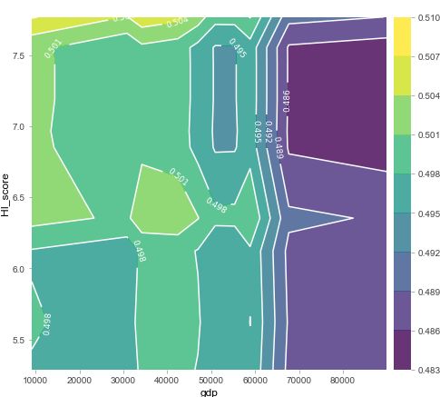
Kijewski, M. et al. /WORKING PAPERS 12/2021 (360)                               3

circular analysis was much more precise than the chance expectations (Herrera, Resa & Sordo,

2010; Baltrunas & Amatriain, 2009).

       Most young people report that they use music to improve their mood, especially when they

are already positive in their initial state. However, some young people reported a deteriorated mood

when feeling sad or stressed. The stressed young people were more likely to listen to intense music

and heavy metal, reporting no more negative impact on their mood than any other music genre

(McFerran et al., 2015; McFerran, 2016). The other study shows completely another view on this

topic. The results suggested that those in sad moods were not unfailingly inclined to listen to sad

songs, but rather were reluctant to listen to happy songs, apparently for fear that the selection of

such songs would seem inappropriate (Friedman, Gordis & Förster, 2012). Another perspective

may also be taken, which suggests that musical preferences reflect mental health rather than

causing it or affecting it. Some studies suggest that musical choices were related to the student's

current academic success or failures, which can affect the choice of music interest (Roe, 1987;

Took & Weiss, 1994). By this fact, we can say that in this area there is no scientific consensus.

       Weather matters, such as the seasons or cloud cover, can define people's musical

preferences, i.e., winter may sometimes isolate individuals and force them to adapt their way of

travel and dress to cope with the changing weather. The research of Pettijohn and Sacco (2009)

showed that more complex music, e.g., instrumental music, is preferable in winter. On the other

hand, in summer preferable is dance music with an emphasis on rhythm emphasized in the genres

of rap/hip-hop, soul/funk, and electronica/dance music (Rentfrow & Gosling, 2003). Application

of the weather and temperature data into the recommendation system caused that evaluation of the

model outperforms the comparative system that utilizes the user’s demographics and behavioral

patterns only (Kim et al., 2008; Lee & Lee, 2007).
Kijewski, M. et al. /WORKING PAPERS 12/2021 (360) 4
Based on the above results from the literature and the preliminary data analysis, we put
forward the following hypotheses:
• Hypothesis 1: Is the effect of summer significant and has a positive effect in the model?
Summertime and vacations are expected to positively influence people’s mood; hence they
tend to listen more happy songs.
• Hypothesis 2: Is the effect of December (Christmas) significant and has a positive effect on
the valence? Christmas is a special time around the world, in this case especially
considering the popularity of Christmas songs, which are full of happiness and love.
• Hypothesis 3: Will the February effect be irrelevant in the model? February is not a month
with any holidays or spikes; thus, we do not expect any difference between February and
other common months.
• Hypothesis 4: Will the effect of the political environment be important in the model? We
assume that a high level of democratization, rule of law, civil liberties, freedom of religion,
freedom of speech and artistic expression will be positively related to the level of valence.
Conversely, as state corruption increases, the relationship should be negative.
• Hypothesis 5: Will the unfavorable socio-economic environment expressed by GDP per
capita, and Happiness Index have a negative impact on valence? It is expected that sad
music is chosen by people who are in a difficult financial situation and happy songs are
listened by cheerful and peaceful people.
• Hypothesis 6: Whether the genre of music has significantly influence valence, i.e., the
variables describing trends in listening will be statistically significant. In general, some
music genres are happier than the others.Kijewski, M. et al. /WORKING PAPERS 12/2021 (360) 5
• Hypothesis 7a: Weather that is forcing people to stay at home negatively affects valence,
i.e., the variable describing cloudiness of the sky will be significant and will have a positive
impact on valence, and that the temperature will have positive impact on valence. It is
expected that current music preferences are affected by the aura. Based on literature, people
are more likely to listen sad music alone, than in groups of people.
• Hypothesis 7b: Weather forcing people to stay at home negatively affects valence, i.e., the
variable assigning countries to specific geographical regions will be statistically significant
and will have negative values for Western Europe, Northern America, Eastern Europe,
Northern Europe, Southern Europe, Eastern Asia, Western Asia, and positive for Latin
America and the Caribbean, Southern Europe.
• Hypothesis 8: Will the results show the effect of more Saturdays per month, i.e., the month
with five Saturdays will have a positive impact on dependent variable. Saturdays are related
to choosing a more positive music vibes, because people are expected to relax over the
weekend and most of the parties are organized on Saturdays. Thus, difference between two
months – one with four Saturdays and the other one with five Saturdays should be visible.
We believe that this article will extend past literature on this topic, by using data of
aggregated choices of individuals with many variables describing current status of the country.
What is more, the results can be a great advice for music business e.g., radio stations or playlist
makers. They can select songs by their positivity using our analysis, which may lead to higher
popularity of the radio or the playlist. The rest of this paper is organized as follows. Section
2 introduces the data set and applied models. Section 3 presents the results. Section 4 consists of
a conclusion and an outlook on potential future research areas.Kijewski, M. et al. /WORKING PAPERS 12/2021 (360) 6
2. Empirical analysis
2.1 Data and variables
The earlier research on the impact of socioeconomic variables on musical preferences has been
more focused on checking whether introducing new information will improve the accuracy of
predicting songs that will be listened to. Whereas we are rather focused on explaining the
phenomenon of trends in listening to the songs with different positivity between months and
countries. We created a dataset with many variables chosen based on the knowledge gathered from
the literature. We believe that this large dataset will allow to obtain more reliable model
architectures than previous datasets. We used Spotify API to create the monthly average valance
dataset for 26 countries for the period from 1 January 2018 to 1 December 2019. Valance describes
the positivity of the song. High valence songs sound more positive (happy, cheerful, euphoric),
while low valence songs sound more negative (sad, depressive, intense). To extend our dataset, we
added monthly aggregated search indices from Google Trends for all the countries describing
trends in music genres (i.e. rap, house, pop, rock, and classical music). To describe democratic
situation of the countries we used Varieties of Democracy (V-Dem) Project (Coppedge et al.,
2020). To explain how diversity of ethnic or religious groups affects selection of the songs based
on positivity, we gathered data from Fractionalization research (Alesina et al., 2003).
For each country we collected 24 variables regarding socio-economic issues, weather and
calendar data aggregated to the monthly level. The descriptions of these features combined with its
basic statistics are summarizes in table 1. It contains the mean, standard deviation (below the mean
in brackets), minimum, 25th quartile, 50th quantile, 75th quartile, and maximum. Our dependent
variable ranges from 0.42 to 0.65. From quantiles and the maximum value, we may conclude thatKijewski, M. et al. /WORKING PAPERS 12/2021 (360) 7
the right tail of the distribution is fat, that exhibits a left skewness and/or high kurtosis. The mean
is equal to 0.4939 and is slightly higher than the median (0.487).
Table 1. Description and summary statistics for variables
Mean 25th 50th 75th
Variable Description Min Max
(sd) Quantile Quantile Quantile
A measure from 0 to 1
describing the musical 0.4939
Valence 0.420 0.468 0.487 0.509 0.652
positiveness conveyed by a (0.041)
track
A happiness index from 6.7140
HI_score 5.287 6.180 6.908 7.332 7.769
World Happiness Report (0.72)
A GDP per capita,
48089.61
Gdp resampled from quarterly 9126.600 36042.525 49640.600 58023.300 89936.300
(16391.56)
to monthly
A variable with a value of
1 if a given month had 5 0.3333
Dancing days 0.000 0.000 0.000 1.000 1.000
Saturdays, and a value of 0 (0.4718)
if it had 4 Saturdays
An ethnic fractionalization
describing probability of 0.2270
Ethnic_frac 0.012 0.103 0.126 0.322 0.712
not belonging to the same (0.1909)
ethnic group
A linguistic
fractionalization
Ling_frac 0.2090
describing the probability 0.000 0.053 0.146 0.323 0.577
(0.1909)
of not belonging to the
same linguistic group
A religious
fractionalization
Relig_frac 0.3926
describing the probability 0.000 0.205 0.353 0.608 0.824
(0.2275)
of not belonging to the
same religious group
A proportion of searches
for classical music on
YouTube to all music
0.4026
Classical categories (Pop, Rock, 0.000 0.209 0.343 0.577 1.000
(0.2686)
Rap, House, Classical),
download and prepared
from Google Trends
A proportion of searches
for pop music on YouTube
0.3882
Pop_music to all music categories, 0.000 0.156 0.315 0.589 1.000
(0.2868)
download and prepared
from Google Trends
A proportion of searches
for rap music on YouTube
0.4306
Rap to all music categories, 0.000 0.205 0.399 0.622 1.000
(0.2770)
download and prepared
from Google TrendsKijewski, M. et al. /WORKING PAPERS 12/2021 (360) 8
A proportion of searches
for rock music on
YouTube to all music 0.5041
Rock 0.000 0.339 0.492 0.678 1.000
categories, download and (0.2566)
prepared from Google
Trends
A proportion of searches
for house music on
YouTube to all music 0.4517
House 0.000 0.246 0.431 0.661 1.000
categories, download and (0.2716)
prepared from Google
Trends
A logarithm of percent of
Sky_log the sky hidden behind the 3.5542
0.338 3.286 3.522 3.839 4.372
clouds, values from 0 to (0.3381)
100
A monthly sum of 164.2558
Sun_hrs 5.000 99.000 162.050 222.750 363.000
sunshine hours (80.1069)
An average monthly 53.6035
Temperature 16.245 42.788 53.598 64.920 83.591
temperature in Fahrenheit (13.99)
A freedom of academic
and cultural expression.
2.2282
v2clacfree Ordinal converted to -2.209 2.182 2.567 2.875 3.212
(1.1238)
interval in the original
dataset.
A freedom of religion
indicating to what extent
individuals are free to
1.6816
v2clrelig choose and practice their -0.661 1.398 1.726 2.090 2.800
(0.7078)
religions. Ordinal
converted to interval in the
original dataset.
A political corruption
index related to frequency
0.1430
v2x_corr of briberies and 0.002 0.021 0.056 0.202 0.765
(0.1992)
embezzlements. Interval
from low to high (0-1)
A categorical variable
indicating to what extent
the electoral democracy 0.8156
v2x_polyarchy 0.279 0.826 0.870 0.881 0.913
applies in the country. (0.1407)
Interval from low to high
(0-1)
A rule of law indicator,
indicating independence,
transparence, equality in
law enforcements, and if 0.8973
v2x_rule 0.201 0.891 0.968 0.987 0.999
actions of the government (0.1773)
in line with the law.
Interval from low to high
(0-1)
A freedom of discussion
index indicating liberty of 0.9041
v2xcl_disc 0.120 0.908 0.953 0.975 0.987
press and media, privilege (0.1646)
to publicly discuss theKijewski, M. et al. /WORKING PAPERS 12/2021 (360) 9
political issues and liberty
of academic and cultural
discourse. Interval from
low to high (0-1),
Rights to private property.
0.9001
v2xcl_prpty Interval from low to high 0.422 0.908 0.930 0.942 0.971
(0.1021)
(0-1)
Source: Own calculations.
For Sky, Temperature and Valence variables, we encountered a few missing observations
for Turkey and Czech Republic, which were replaced with average for country subregion group.
There were few factors with yearly or quarterly frequency – GDP, Happiness index, fractional and
political variables (v2) for which we replaced missing observations with last known value.
Additionally, we used min-max scaler for trends in music genres.
One variable, Subregion, which assigns a country to a given region, was not described in
the table due to its categorical character. We identified 8 regions, i.e. Western Europe (6 countries),
Northern America (Canada and USA), Eastern Europe (4 countries), Northern Europe (7
countries), Southern Europe (4 countries), Eastern Asia (Japan), Latin America and the Caribbean
(Mexico), and Western Asia (Turkey).
Probability density function of Valence has been estimated using Kernel Density Estimate
(KDE). The estimation results along with the histogram are presented in figure 1. Its fragment, i.e.,
from 0.40 to 0.55, resembles the normal distribution. However, the right tail is fat. To understand
where the reasons behind this phenomenon the valence values above 0.55 were analyzed. There
were 53 observations, so almost 10% of the sample. Most of the records come from Spain and
Mexico. Importantly, all 24-month observations for Mexico exceeded this threshold, and in case
of Spain almost all - 21 out of 24 observations. In addition, six observations come from Japan and
two from Finland.Kijewski, M. et al. /WORKING PAPERS 12/2021 (360) 10
Figure 1. Kernel Density Estimate (KDE) plot with histogram for Valence
Source: Own calculations.
Figure 2 shows how valence changes over time. December stands out here for both years.
Therefore, we can expect the hypothesis for this effect to be confirmed. For 2019, the summer
effect may be noticeable, but for 2018 it is not very visible. What is more, from figure 2. analysis
we cannot see that February stands out with lower valence. As it has similar levels to nearest
months – January and March.Kijewski, M. et al. /WORKING PAPERS 12/2021 (360) 11
Figure 2. Valence probability density over the time segregated from the most recent (at the top)
to the oldest (at the bottom)
Source: Own calculations.
Figure 3 shows how the values of valence percentiles change over time. Here, the December
effect is also clearly visible, which is interesting that it appears not only on the average level but
also applies to every percentile. The summer effect (July and August) is clearly visible, although
what we have expected earlier, the effect is much more visible for 2019. In 2018, the effect was
observable only for the 90th percentile. Thus, countries that listen to happy music for most of the
time in the year, are listening to even happier music in summer in comparison to other countries.Kijewski, M. et al. /WORKING PAPERS 12/2021 (360) 12
Figure 3. Quantile trend plot for Valence
Source: Own calculations.
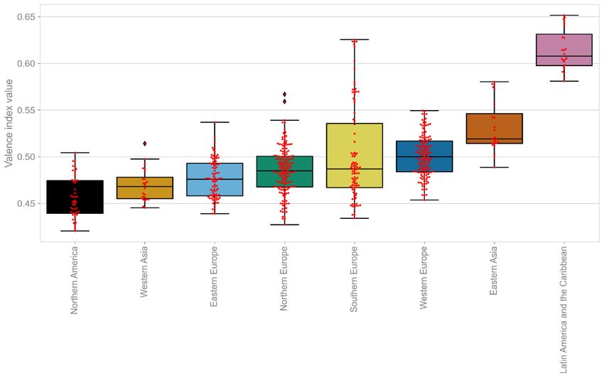
Figure 4 shows the valence in individual regions. Southern Europe, Latin America and the
Caribbean stand out clearly from other regions. In both regions, Spotify users listen to much more
positive music.
Figure 4. Valence in particular subregions
Source: Own calculations.Kijewski, M. et al. /WORKING PAPERS 12/2021 (360) 13
Figure 5 shows the correlation between the variables. The most closely related variables are
the political variables, i.e. v2clacfree, v2clrelig, v2x_corr, v2x_rule, v2xcl_prpty, v2c_polyarchy,
and v2xcl_disc. The correlation between valence and the explanatory variables can be assessed as
moderate (it ranges from 0.2 to 0.5).
Figure 5. Correlation between the variables used in the research
Source: Own calculations.Kijewski, M. et al. /WORKING PAPERS 12/2021 (360) 14 2.2 Empirical design 2.2.1 Panel Data Regression Model The data used in this research is a panel with 26 countries serving as groups and 24 monthly observations for each variable, hence the most obvious choices are panel data regression models with fixed effects and random effects. For the purpose of determining the proper estimator, we used the Hausman test which null hypothesis points towards using a random effects estimator and the alternative hypothesis indicates that the random effects estimates are inconsistent and hence fixed effects estimator should be chosen. The results of the Hausman test indicated that the null hypothesis is rejected, and hence the fixed effects (FE) panel regression should be used. In order to come up with a set of significant variables for regression analysis we applied General-to-Specific modelling procedure (Campos, Ericsson & Hendry, 2005), which consists of iterative model estimation, dropping the variable with the highest p-value of the significance test and testing the joint hypothesis of insignificance of the dropped variables. 2.2.2 Dynamic Panel Data Regression Model Dynamic panel data regression models are used in cases where the autoregressive process of the dependent variable is significant, hence its future values depend on the past. To test this assumption we tested significance of AR(1) process of the dependent variable. The results strongly rejected the null hypothesis of insignificance and hence indicated that the autoregressive term is not redundant in explaining the regressand. Therefore, we concluded that it is necessary to include the lagged values of the dependent variable in the panel. The rationale behind this model is also the retention in music taste and the fact that people generally tend to listen a specific type of music for a longer period as well as come back to the songs they enjoyed listening recently. In such case using fixed
Kijewski, M. et al. /WORKING PAPERS 12/2021 (360)                              15

effects regression model will lead to the Nickell’s bias and the estimated coefficients will be

inaccurate, especially in the context of panels with small T and large N. This bias arises due to

exclusion of individual fixed effect from each observation, which in case of including the lagged

regressor leads to introducing correlation between the regressors and the error term. Since the panel

used in this research is relatively short, as it consists of only 24 monthly observations, we have

decided to use Arellano and Bover / Blundell and Bond system estimator, which is unbiased and

effective for dynamic panel data even in a small sample. Consistently with previous panel

regression model, General-to-Specific modelling approach was applied to select the set of

significant variables.

2.2.3 CatBoost model and Explainable Artificial Intelligence

To analyze the research problem in depth, we also applied the CatBoost model (Prokhorenkova et

al., 2017) in its classic regression form. That is, we entered panel data into the model, and the

machine learning estimator treats them as cross-sectional data. Importantly, we have chosen not to

consider the specificity of the time series in this model in order to simplify the estimation and

statistical inference process.

       The biggest advantage of the boosting trees model in our context is a lack of assumption

regarding the linear function, thus it can handle highly non-linear interactions in the data. We are

aware that manual search for an appropriate polynomial or power functional form for the linear

panel approach like fixed-effects model usually fails due to a vast space of possible solutions. What

is more, boosting schemes applied in CatBoost allowed us to control variance (overfitting) in

a responsible way. In addition, CatBoost perfectly model highly cardinal variables (we have such

in the analysis). Importantly, the CatBoost model interpretation is not as trivial as for FE or DPD.
Kijewski, M. et al. /WORKING PAPERS 12/2021 (360) 16
However, it is feasible with techniques such as feature importance and feature effects powered by
SHapley Additive exPlanations (Lundberg & Lee, 2017).
Our CatBoost modelling process was relatively straightforward. We searched for the best
hyperparameters in a 5-folded cross-validation grid search with following setup (based on our
experience): depth [2, 3, 4, 5, 6, 7], learning rate [0.01, 0.05, 0.1, 0.25, 0.5], iterations [50, 100,
150, 200, 250, 300]. During this process, our evaluation metric was root mean squared error.
Feature importance techniques enable us to analyze the significance of a given variable
throughout the model and determine its quasi-participation in the predictive power of the model.
SHapley Additive exPlanations (SHAP) is a game theoretic approach to explain the output of any
machine learning model. As we were focused on summarizing the effects of all the features, we
used SHAP summary plot. It sorts features by the sum of SHAP value magnitudes over all samples
and uses SHAP values to show the distribution of the impact each feature has on the model output.
The color represents the feature value (red for high, blue for low). What is more, we used SHAP
Partial Dependence Plot (2D partial Partial Dependence Plot) to examine the overall effect of
a single feature (of two features) across the whole dataset. This kind of plots represents a change
in dependent variable as independent variable changes.
3. Results
3.1 Fixed effects panel model
After conducting General-to-Specific approach, the finally obtained model for fixed effects has 11
independent variables, 10 of the variables are significant at the level of at least 0.1 and 8 of them
are significant at the level of at least 0.05. The values of coefficients, standard errors, and p-value
are reported in the table 2.Kijewski, M. et al. /WORKING PAPERS 12/2021 (360) 17
Table 2. Coefficients, standard errors, and p-value for Panel Data Regression Models
Variable Model 1 Model 2 Model 3
Temperature 0.0002 0.00012 -
(0.0002) (0.0001)
Gdp 0.000003* 0.000003* 0.000003*
(1.14e-06) (1.16e-06) (1.12e-06)
HI_score -0.03021 -0.02816 -0.033
(0.019) (0.0191) (0.0197).
V2clrelig 0.01314* 0.0139* 0.014854*
(0.0063) (0.0058) (0.006)
V2x_corr -0.35842*** -0.33093*** -0.33766***
(0.0466) (0.0559) (0.0556)
V2xcl_prpty 0.13198 - -
(0.0975)
Classical 0.00675 0.00733 0.00636
(0.0037). (0.0039). (0.00397)
House 0.00016*** 0.011896*** 0.01355***
(0.0032) (0.00316) (0.0031)
Rap -0.01212*** -0.01446*** -0.01586***
(0.0041) (0.00379) (0.00343)
Pop_music 0.0068129 0.0078 0.008
(0.0045155) (0.00459). (0.0048).
Dancing_days 0.00381*** 0.00376*** 0.00435***
(0.0005) (0.0005) (0.00055)
Summer 0.00787*** 0.00804*** 0.0104***
(0.00124) (0.00127) (0.00169)
Xmas 0.01584*** 0.015869*** 0.0139***
(0.0035) (0.00346) (0.00344)
Source: Own calculations.
This model strongly confirms the hypotheses 1, 2, and 3 about the importance of the
summer and December effects and not significant February effect. Hypothesis 4 has been partially
confirmed. Only variables regarding freedom of religion (v2clrelig) and political corruption
(v2x_corr) are statistically significant. Hypothesis 5 has been confirmed. Variable gdp is significant
and is positive, but surprisingly HI_score is not significant. It may be caused by correlation
between HI_score and gdp. Hypothesis 6 has been partially confirmed. The impact of the house,
rap, and pop has been confirmed. For the house and pop music effects are positive, while for rap itKijewski, M. et al. /WORKING PAPERS 12/2021 (360) 18
is negative. Hypotheses 7a and 7b have been fully rejected. The variables temperature and sky are
not statistically significant. Hypothesis 8 has been confirmed. The variable dancing_days is
significant and positive.
3.2 Arellano and Bover / Blundell and Bond system estimator
Table 3. Coefficients, standard errors, and p-values for Arellano and Bover / Blundell and Bond
system estimator
Model 1 Model 2 Final model
Variable
A-B / B-B A-B / B-B A-B / B-B
Lag.Valence 0.6280*** 0.632*** 0.623***
(0.0276) (0.027) (0.0264)
Temperature 0.00038*** 0.0004*** 0.00036***
(0.000055) (0.00004) (0.0004)
Gdp -7.90 e-07*** -7.69 e-07** -7.61 e-07**
(3.13 e-07) (3.14 e-07) (3.31 e-07)
HI_score 0.0232*** 0.023*** 0.0225***
(0.0056) (0.0056) (0.0056)
V2clrelig 0.0139*** 0.0135*** 0.01425***
(0.0033) (0.0034) (0.0.033)
V2x_polyarchy 0.1511*** 0.15*** 0.1495***
(0.0421) (0.042) (0.0422)
V2xcl_disc -0.1810*** -0.178*** -0.1795
(0.035) (0.035) (0.035)
Log_sky 0.0041 0.004 -
(0.0037) (0.03)
House 0.0071*** 0.007*** 0.0071***
(0.0.018) (0.0018) (0.0018)
Rap -0.0028* -0.0029* -0.0032**
(0.0018) (0.0019) (0.0018)
Pop_music 0.00921*** 0.0091*** 0.0094***
(0.0017) (0.0017) (0.0017)
Dancing_days 0.0047*** 0.0046*** 0.0045***
(0.00077) (0.00078) (0.0007)
Summer 0.0011 - -
(0.0011)
Xmas 0.022*** 0.022*** 0.022***
(0.0014) (0.0014) (0.001)
Sun_hours 0.000024*** 0.000023*** 0.00002***
(0.0000065) (0.0000065) (0.0000068)Kijewski, M. et al. /WORKING PAPERS 12/2021 (360) 19
Ethnic_fraction 0.1546*** 0.1545*** 0.1578***
(0.0253) (0.0254) (0.0253)
Lingual_fraction -0.228*** -0.227*** -0.228***
(0.03599) (0.036) (0.218)
Relig_fraction 0.089*** 0.088*** 0.087***
(0.0212) (0.022) (0.0218)
Source: Own calculations.
In table 3. we presented the results from Arellano and Bover / Blundell and Bond system
estimator on dynamic panel data. In the table we showed the only last three iterations of General-
to-Specific approach. All independent variables were significant at 5% level of confidence in our
final model. The autoregressive process was significant, which confirms the usage of Dynamic
Panel Data estimators. Retention rate is almost 63% for valence. Temperature and number of sun
hours has positive impact on valence, which confirms the 7th hypothesis that the bad weather forces
people to stay at home, which can lead to lower valence levels. In contradiction to the FE model,
GDP has negative impact on valence. In countries with favorable political environment (v2clrelig,
v2x_polarchy) we can expect higher valence. Variables describing trends of music genre are also
statistically significant for house, rap and pop music. Only rap music has negative impact on
valence, which is in line with intuition that rap music tends to be negative. Number of Saturdays
in a month has a positive impact on dependent variable, which suggest that Saturday itself has
significant impact. Next, we wanted to check, if the second and the third hypotheses were
confirmed. February dummy was insignificant, which confirms third hypothesis. We also observed
a positive significant impact of Christmas dummy, however variable flagging summer was
insignificant.
To confirm the proper selection of the instruments, we calculated Arellano-Bond test. Test
confirms proper form of the model, as we expected the autocorrelation of first order – the testKijewski, M. et al. /WORKING PAPERS 12/2021 (360) 20 rejects the null hypothesis for zero autocorrelation in first-differenced error and for second order we cannot reject null hypothesis at 5% level of confidence (p-value is equal to 0.861). 3.3 CatBoost model Our final CatBoost model gathered 22 explanatory variables. Based on cross-validation (described in the methodology subsection), we set following hyperparameters values: iteration 250, learning rate 0.1 and tree depth 3. The general results of the model obtained using SHAP Summary Plot are presented in the figure 6. It clearly shows that variables like subregion, rock, GDP, rap, month of the year, house and temperature are the most important for this discriminative model. We see that variables generally affect model’s output in expected way. But to be more specific, we propose to analyze SHAP Partial Dependence Plots for exogenous features. These plots are visualized in the figure 7 (note the different scale of the ordinate axis). Figure 6. SHAP Summary Plot based on CatBoost model Source: Own calculations.
Kijewski, M. et al. /WORKING PAPERS 12/2021 (360)                               21

       Let us first analyze the influence of music genres. We can easily conclude that the greater

popularity of pop, house, rock in each country, the greater the valence. The effect of rap is strictly

negative, while the popularity of classical music only has a measurable positive effect on the

expected value of the target variable from a certain point onwards. In the case of meteorological

variables, temperature has a clearly monotonic positive effect on valence, and the logarithmical

cloudiness of the sky is not relevant to the model at all. The effect of sunshine hours seems to be

positively significant only for the extreme values of this exogenous variable. For the months,

valence is positively influenced by the holiday period (June to September) and Christmas

(December). The impact of other months is insignificant. Dancing days have a positive impact on

the target variable. The impact of the Happiness index is unclear. An interesting finding is that

countries with low and medium GDP per capita have higher expected valence than the richest

countries. Jointly, the political and constitutional variables do not clearly indicate their impact on

the explanatory variable. However, the rule of law, rights to private property, and freedom of

religion have a very positive influence on the outcome of the model. An interesting effect has the

freedom of discussion index, which for the largest value has a negative effect on the fitted value

from the model. The higher the religious and ethnic diversity, the more we expect the valence to

be positively affected. Linguistic diversity to some extent suggests a similar relationship. The

subregion variable is hard to interpret due to its poor balancing, while it shows that subregions are

strongly homogeneous with respect to the target variable.
Kijewski, M. et al. /WORKING PAPERS 12/2021 (360) 22 Figure 7. SHAP Partial Dependence Plots based on CatBoost model
Kijewski, M. et al. /WORKING PAPERS 12/2021 (360)   23

Source: Own calculations.
Kijewski, M. et al. /WORKING PAPERS 12/2021 (360)                                 24

       In addition, we used SHAP 2D Partial dependence plots to interpret the CatBoost results

(see figure 8). In this case, the pairs of variables of our interest are pop_music – rap, sun_hours –

temperature and HI_score - gdp. We decided to test the main effect of each feature and their

interaction effect. Based on these graphs, we can confirm the earlier conclusions of the 1D PDP,

i.e. the popularity of rap has a negative effect on valence, while pop has a positive effect. Altogether

we can see that even a relatively low popularity of rap, with a high popularity of pop strongly

negatively affects the final valence. When it comes to the relationship between temperature and

days of sunshine, temperature is clearly the key. Sunny days create a bulge in the graph, i.e. despite

high temperature, few sunny days will lower the expected value of the target variable. A very

interesting relationship is shown by the Happiness Index and GDP. It turns out that the highest

expected valence is in countries with relatively low income and high Happiness Index. Moreover,

moderate Happiness Index and average GDP also lead to above average valence.

Figure 8. SHAP 2D Partial Dependence Plots based on CatBoost model
Kijewski, M. et al. /WORKING PAPERS 12/2021 (360) 25
Source: Own calculations.
To sum up, the two models fully confirmed the hypothesis 1, 2 and 3. Only the Dynamic
Panel Data Regression Model did not confirm the summer effect. In the context of hypothesis 4,
all models confirmed the significance of freedom to religion (v2clrelig). Two models confirmed
the significance of the political corruption index (v2x_corr), the electoral democracy
(v2c_polyarchy), religious diversity (relig_frac) and ethnic diversity (ethnic_frac). Hypothesis
5 for gdp was confirmed, although this variable had the opposite effect to that predicted. For the
Dynamic Panel Data Regression Model and CatBoost, it was negative, for the fixed effects model
the gdp impact is positive. All models partially confirmed hypothesis 6. House and pop had
a positive effect on the valence, while the rap negative. Only the CatBoost model confirmed the
added impact of rock. All models refuted hypotheses 7a with regard to the significance of cloud
cover (sky_log). In case of hypothesis 7b subregions were strongly significant only for CatBoost
model (it can utilize very well highly cardinal variables). All models confirmed the significance
and a positive coefficient for the variable dancing_days, which confirmed the last hypothesis 8.Kijewski, M. et al. /WORKING PAPERS 12/2021 (360) 26
4. Conclusions
The models allowed to confirm most of the hypotheses put forward at the beginning. These results
are important as much as they contradicted the conclusions drawn by The Economist that February
would be the gloomiest month in terms of the music listened to. The remaining effects may broaden
the artists' knowledge of when to release new songs. Streaming services such as Spotify may be
another beneficiary of the results. The recommendation engines for songs and playlists could be
more accurate if they also considered the variables we added.
The first limitation of this study is that valence may be largely related to the kinds of music.
Therefore, further research should focus on the analysis of disaggregated data and a possible
valence comparison for given genres of music. The distribution of valence at the country level
could also be interesting. The analysis of the mean alone does not provide all information about
the mood of the music being listened to, there is a possibility that distribution can be bimodal –
people can listen to extremely negative and extremely positive music. Additionally, the influence
of political variables is unclear. There is no theoretical basis for the interpretation of the obtained
results based on theories from the literature. Another limitation is the short period of the analyzed
data. Two years do not allow to properly capture the seasonality, which was our main interest in
the third hypothesis. Another limitation is the lack of monthly macroeconomic and social data. For
this reason, some of the variables in our analysis had only two unique values.Kijewski, M. et al. /WORKING PAPERS 12/2021 (360) 27
References
Alesina, A., Devleeschauwer, A., Easterly, W., Kurlat, S., & Wacziarg, R. (2003).
Fractionalization. Journal of Economic growth, 8(2), 155-194.
https://doi.org/10.1023/A:1024471506938
Baltrunas, L., & Amatriain, X. (2009). Towards time-dependent recommendation based on
implicit feedback. In Workshop on context-aware recommender systems, 25 - 30.
Campos, J., Ericsson, N. R., & Hendry, D. F. (2005). General-to-specific modeling: an
overview and selected bibliography. FRB International Finance Discussion Paper, 838.
Coppedge, M., Gerring, J., Knutsen, C. H., Lindberg, S. I., Teorell, J., Altman, D., Ziblatt,
D. et al. (2020). V-dem Dataset v10. Varieties of democracy (V-Dem) Project.
https://doi.org/10.23696/vdemds20
Herrera, P., Resa, Z., & Sordo, M. (2010). Rocking around the clock eight days a week: an
exploration of temporal patterns of music listening. In 1st Workshop On Music Recommendation
And Discovery, ACM RecSys, 2010, Barcelona, Spain.
Friedman, R. S., Gordis, E., & Förster, J. (2012). Re-exploring the influence of sad mood
on music preference. Media Psychology, 15(3), 249 - 266.
https://doi.org/10.1080/15213269.2012.693812
Hospers, J. (1969). Introductory readings in aesthetics. Free Press.
Kellaris, J. J. (2008). Music and consumers in Haugtvedt, C. P., Herr, P. M., & Kardes, F.
R. (Eds.). (2018). Handbook of consumer psychology, 837 - 856. Routledge.
Kim, J.-H., Jung, K.-Y., Ryu, J.-K., Kang, U.-G., & Lee, J.-H. (2008). Design of ubiquitous
music recommendation system using MHMM. In Int. Conf. on Networked Computing and
Advanced Information Management, 2, 369 - 374.Kijewski, M. et al. /WORKING PAPERS 12/2021 (360) 28
Lai, H. L. (2004). Music preference and relaxation in Taiwanese elderly people. Geriatric
Nursing, 25(5), 286 - 291. https://doi.org/10.1016/j.gerinurse.2004.08.009
Lee, J. S., & Lee, J. C. (2007). Context awareness by case-based reasoning in a music
recommendation system. In International symposium on ubiquitious computing systems, 45-58.
Springer, Berlin, Heidelberg. https://doi.org/10.1007/978-3-540-76772-5_4
Levinson, J. (1997). Music and negative emotion. In J. Robinson (Ed.), Music and meaning
(215-241). Ithaca, NY: Cornell University Press.
Liu, M., Hu, X., & Schedl, M. (2018). The relation of culture, socio-economics, and
friendship to music preferences: A large-scale, cross-country study. PloS one, 13(12).
Lundberg, S.M. and Lee, S. (2017). A Unified Approach to Interpreting Model Predictions,
Advances in Neural Information Processing Systems, 30, 4765-4774.
McFerran, K. S., Garrido, S., O’Grady, L., Grocke, D., & Sawyer, S. M. (2015). Examining
the relationship between self-reported mood management and music preferences of Australian
teenagers. Nordic Journal of Music Therapy, 24(3), 187 - 203.
https://doi.org/10.1080/08098131.2014.908942
McFerran, K. S. (2016). Contextualising the relationship between music, emotions and the
well-being of young people: A critical interpretive synthesis. Musicae Scientiae, 20(1), 103-121.
https://doi.org/10.1177/1029864915626968
Mellander, C., Florida, R., Rentfrow, P. J., & Potter, J. (2018). The geography of music
preferences. Journal of Cultural Economics, 42(4), 593 - 618. https://doi.org/10.1007/s10824-018-
9320-x
Pettijohn, T. F., II, & Sacco, D. F., Jr. (2009). Tough times, meaningful music, mature
performers: popular Billboard songs and performer preferences across social and economicKijewski, M. et al. /WORKING PAPERS 12/2021 (360) 29
conditions in the USA. Psychology of Music, 37, 155 - 179.
https://doi.org/10.1177/0305735608094512
Prokhorenkova, L., Gusev, G., Vorobev, A., Dorogush, A. V., & Gulin, A. (2017).
CatBoost: unbiased boosting with categorical features. arXiv preprint arXiv:1706.09516.
Rentfrow, P., Mellandar, C., Florida, R., Hracs, B. J., & Potter, J. (2013). The geography
of music preferences.
Rentfrow, P. J., & Gosling, S. D. (2003). The do re mi’s of everyday life: the structure and
personality correlates of music preference. Journal of Personality and Social Psychology, 84, 1236
- 1253. https://doi.org/10.1037/0022-3514.84.6.1236
Roe, K. (1987). The school and music in adolescent socialisation. In J. Lull (Ed.), Pop music
and communication, 212–230. Thousand Oaks, CA: Sage.
Skowron, M., Lemmerich, F., Ferwerda, B., & Schedl, M. (2017). Predicting genre
preferences from cultural and socio-economic factors for music retrieval. In European Conference
on Information Retrieval, 561 - 567. Springer, Cham. https://doi.org/10.1007/978-3-319-56608-
5_49
Schedl, M., Lemmerich, F., Ferwerda, B., Skowron, M., & Knees, P. (2017). Indicators of
country similarity in terms of music taste, cultural, and socio-economic factors. In 2017 IEEE
International Symposium on Multimedia (ISM), 308 - 311. IEEE.
https://doi.org/10.1109/ISM.2017.55
Scherer, K. R. (2004). Which emotions can be induced by music? What are the underlying
mechanisms? And how can we measure them?. Journal of new music research, 33(3), 239-251.
https://doi.org/10.1080/0929821042000317822Kijewski, M. et al. /WORKING PAPERS 12/2021 (360) 30
The Economist. (2020). Data from Spotify suggest that listeners are gloomiest in February.
The Economist. https://www.economist.com/graphic-detail/2020/02/08/data-from-spotify-
suggest-that-listeners-are-gloomiest-in-february
Took, K. J., & Weiss, D. S. (1994). The relationship between heavy metal and rap music
on adolescent turmoil: Real or artifact? Adolescence, 29, 613 - 621.
Vigliensoni, G., & Fujinaga, I. (2016). Automatic Music Recommendation Systems: Do
Demographic, Profiling, and Contextual Features Improve Their Performance?. In ISMIR, 94-100.
Vlegels, J., & Lievens, J. (2017). Music classification, genres, and taste patterns: A ground-
up network analysis on the clustering of artist preferences. Poetics, 60, 76 - 89.
https://doi.org/10.1016/j.poetic.2016.08.004
Vuoskoski, J. K., Thompson, W. F., McIlwain, D., & Eerola, T. (2011). Who enjoys
listening to sad music and why?. Music Perception, 29(3), 311 - 317.
https://doi.org/10.1525/mp.2012.29.3.311UNIVERSITY OF WARSAW FACULTY OF ECONOMIC SCIENCES 44/50 DŁUGA ST. 00-241 WARSAW WWW.WNE.UW.EDU.PL
You can also read