Occasional Paper Series - Fiscal expenditure spillovers in the euro area: an empirical and model-based assessment - European ...

Occasional Paper Series
 Mario Alloza, Marien Ferdinandusse, Fiscal expenditure spillovers
 Pascal Jacquinot, Katja Schmidt
 in the euro area:
 an empirical and model-based
 assessment

 No 240 / April 2020

Disclaimer: This paper should not be reported as representing the views of the European Central Bank (ECB).
The views expressed are those of the authors and do not necessarily reflect those of the ECB.

Contents
Abstract 2

Executive summary 3

1 Introduction 4

2 Empirical estimates of government spending spillovers in the euro
 area 7

 2.1 PVAR estimates of government spending spillovers 7

 2.2 Structural vector autoregression estimates of government
 spending spillovers 12

3 Spillover analysis based on a multi-country DSGE model 19

 3.1 Spillovers with reactive and non-reactive monetary policy 21

 3.2 Sensitivity analysis 23

4 Conclusions 26

References 28

Appendix 31

ECB Occasional Paper Series No 240 / April 2020 1

1 Abstract

 The paper describes the main transmission channels of the spillovers of national fiscal
 policies to other countries within the euro area and investigates their magnitude using
 different models. In the context of Economic and Monetary Union (EMU), fiscal
 spillovers are relevant for the accurate assessment of the cyclical outlook in euro area
 countries, as well as in the debates on a coordinated change in the euro area fiscal
 stance and on a euro area fiscal capacity. The paper focuses on spillovers from
 expenditure-based expansions by presenting two complementary exercises. The first
 is an empirical investigation of spillovers based on a new, long quarterly dataset for
 the largest euro area countries and on new estimates based on annual data for a
 panel of 11 euro area countries. The second uses a multi-country general equilibrium
 model with a rich fiscal specification and the capacity to analyse trade spillovers.
 Fiscal spillovers are found to be heterogeneous but generally positive among euro
 area countries. The reaction of interest rates to fiscal expansions is an important
 determinant of the magnitude of spillovers.

 Keywords: fiscal spillovers, fiscal policy, monetary policy, VAR, DSGE.

 JEL codes: F42, F45, H50, E62, E63

 ECB Occasional Paper Series No 240 / April 2020 2

2 Executive summary

 Fiscal spillovers across countries have received increasing attention in recent
 years. Understanding the impact of one country’s fiscal policies on output in other
 Member States of the monetary union is of interest to a central bank setting a single
 monetary policy, as this feeds into the assessment of the risks to price stability. Fiscal
 spillovers should also be taken into account when assessing the aggregate euro area
 fiscal stance. Finally, the size of the fiscal spillovers is important when assessing the
 stabilisation effects of national fiscal policies. If the fiscal spillovers are small, then the
 existence of a central fiscal stabilisation function that can support national economic
 stabilisers in the presence of large economic shocks would make Economic and
 Monetary Union (EMU) more resilient.

 This paper provides new estimates – based on a suite of models – of fiscal
 expenditure spillovers in the euro area, as well as simulations to promote a
 better understanding of their driving factors. Our first empirical approach consists
 of an estimate of the average spillover effect among euro area countries, using a panel
 vector autoregressive model. The second approach focuses on the individual
 spillovers among the four largest euro area countries using vector autoregressive
 models. Finally, a multi-country DSGE model that was specifically calibrated to
 simultaneously analyse the four largest euro area countries is used to investigate the
 factors influencing the magnitude of fiscal spillovers, in particular the interaction with
 monetary policy.

 The empirical results confirm the existence of positive fiscal spillovers within
 euro area countries. New estimates based on a panel of euro area countries with
 annual data, as well as new estimates for the four largest euro area countries
 individually that are based on a new quarterly dataset, confirm the findings of earlier
 studies that fiscal expenditure has positive spillovers across countries.

 The reaction of interest rates is an important determinant of the magnitude of
 spillovers. The dynamic stochastic general equilibrium (DSGE) model simulations
 illustrate that the composition of government expenditure has implications for the
 magnitude of spillovers, with productive government investment providing larger
 spillovers than consumption. The model simulations also explore the relationship
 between the reaction of interest rates and spillovers, as the empirical results suggest
 that spillovers are higher when interest rates react less to the government expenditure
 shock.

 All in all, spillovers within the euro area are higher when interest rates are not
 increased in response to an increase in government expenditure, but remain
 below the domestic impact of fiscal expenditure. This suggests that fiscal
 spillovers could play a greater stabilising role in the euro area cycle if the efficacy of
 monetary policy instruments is less than during normal times.

 ECB Occasional Paper Series No 240 / April 2020 3

3 Introduction

 Fiscal spillovers across countries have received increasing attention in recent
 years. Understanding the impact of a country’s fiscal policies on output in other
 Member States of the monetary union is naturally of considerable interest to a central
 bank setting a single monetary policy. This allows the bank to better gauge the euro
 area’s economic developments, and in turn feeds into the assessment of risks to price
 stability. Moreover, fiscal spillovers should be taken into account when assessing the
 aggregate euro area fiscal stance. Finally, the size of fiscal spillovers is important
 when assessing the stabilisation effects of national fiscal policies. If fiscal spillovers
 are small, then the existence of a central fiscal stabilisation function that can support
 national economic stabilisers in the presence of large economic shocks would make
 EMU more resilient.

 National fiscal policies spill over to other countries through different channels.
 Trade is an important transmission channel between countries, whereby a fiscal
 expansion in one country increases its imports from other countries. Fiscal expansion
 could also increase domestic prices and the real effective exchange rate, reinforcing
 spillovers, as the stimulating country loses competitiveness vis-à-vis the other
 countries. Given the implications for prices, it is important to take into account the
 monetary policy response. Interest rates may occasionally fail to react to price
 changes stemming from fiscal action, for instance, if the economy is constrained by
 the effective lower bound.

 This paper provides new estimates of fiscal spillovers in the euro area and
 simulations using a suite of multi-country models to better understand the
 driving factors. Our first empirical approach consists of an estimate of the average
 spillover effect among 11 euro area countries, using a panel vector autoregression
 (PVAR) model based on annual data since 1972. The second approach focuses on
 the individual spillovers among the four largest euro area countries, using VAR models
 which are based on a new quarterly dataset. Comparing up-to-date estimates based
 on different data and using different estimation methods enhances the robustness of
 our findings. By employing a multi-country DSGE model that was specifically
 calibrated to analyse the four largest euro area countries simultaneously, we are able
 to investigate the factors influencing the magnitude of fiscal spillovers, in particular
 their interactions with monetary policy. Both the empirical estimates and the DSGE
 simulations focus on an expenditure-based fiscal expansion.

 The empirical literature on fiscal spillovers is relatively underdeveloped. While
 the number of empirical studies estimating the size of fiscal spillovers has grown in
 recent years, it is limited, and results are not easily comparable. The differing
 identification of fiscal shocks and presentation of the results according to different
 metrics makes generalising the findings from the literature all the more complex. In
 addition, there are few papers that focus on the euro area.

 Spillover estimates of public spending tend to be positive but generally small. A
 number of studies have estimated fiscal spillovers from an increase in public spending

 ECB Occasional Paper Series No 240 / April 2020 4

through the trade channel for a panel of countries. For example, based on annual data
from 1965 to 2004, Beetsma et al. (2006) estimate that a spending-based fiscal
expansion of 1% of GDP in Germany would lead to an average increase in the output
of other EU economies by 0.15% after two years; for an expansion originating in
France, the impact is 0.08%. Using quarterly data from 2000 to 2016 for 55 countries,
the International Monetary Fund (IMF) reports that an increase in government
spending by 1% of GDP in an average major advanced economy has a spillover effect
of 0.15% of GDP on an average recipient country within the first year (IMF (2017) and
Blagrave et al. (2017)). When restricting the sample to Europe, the IMF estimates the
one-year spillover of 1% government spending shock in Germany and in France to be
0.26% and 0.14%, respectively (Blagrave et al. (2017)). Auerbach and Gorodnichenko
(2013), who in contrast to the abovementioned studies normalise spillovers to the
recipient country’s GDP, find fiscal spillovers from large OECD economies that are
broadly comparable with the IMF’s findings (see Annex 6 in Blagrave et al. (2017) for a
comparison).

Spillover estimates are heterogeneous. The estimated magnitude of spillovers
varies, with the heterogeneity related to the trade links, the state of the economy and
the reaction of monetary policy. Beetsma et al. (2006) find spillovers from Germany to
be around 0.4% of GDP after two years in small open economies sharing a land
border with the country, such as Austria, Belgium and the Netherlands. Auerbach and
Gorodnichenko (2013) find spillovers that are particularly high in recessions and more
modest in expansions. 1 The IMF study finds that spillovers are up to four times as
large when monetary policy is at the effective lower bound (0.3% after one year),
compared with normal times (0.08%).

Additional insight into fiscal spillovers is provided by a number of studies
using theoretical DSGE models. Rich DSGE multi-country models can provide more
insight into the determinants of the fiscal spillovers than empirical methods such as
vector auto-regressions (VARs), which encompass a variety of contributing effects
that are difficult to disentangle. 2 However, DSGE models may come at the price of
imposing restrictive assumptions, which may not always have strong empirical
foundations. Studies based on DSGE models often find spillovers in normal times to
be lower than the VAR-based estimates, but higher when interest rates do not react.
This is partly explained by the fact that structural models only include spillovers
through trade, whereas VARs also include other effects, such as financial spillovers.

Throughout the paper, spillovers are summarised by destination and by origin.
Destination spillovers measure the spillover from a spending shock, in all but one euro
area country, on the recipient country. This gives an indication of the effect of a
simulaneous fiscal stimulus among euro area Member States. Spillover by origin is the

1
 For domestic fiscal multipliers, the findings by Auerbach and Gorodnichenko (2012) of higher multipliers
 in recessions have been shown to be fragile to small changes in specification (see, for example, Alloza
 (2017)). In an overview paper of the effects of fiscal policy, Ramey (2019) concludes that “most estimates
 of government spending multipliers for general categories of government spending for averages over
 samples are in the range of 0.6 to 0.8, or perhaps up to 1. The evidence for multipliers above one during
 recessions or times of slack is typically not robust. However, some initial explorations suggest that
 government spending multipliers could be higher at times when monetary policy accommodates fiscal
 policy, such as during periods at the zero lower bound of interest rates or wartime”.
2
 Examples are In ‘t Veld (2017) and Blagrave et al. (2018).

ECB Occasional Paper Series No 240 / April 2020 5

impact on the output in the receiving countries of fiscal action in one country. This
statistic indicates the magnitude of the spillovers that an individual country is able to
generate. In Chapter 2, the empirical results are presented, followed by a chapter
demonstrating the DSGE model simulations. Chapter 4 concludes the paper.

ECB Occasional Paper Series No 240 / April 2020 6

4 Empirical estimates of government
 spending spillovers in the euro area

 This section presents new estimates of fiscal spillover effects from the euro area
 countries. To this end, country-specific exogenous government spending shocks are
 identified and their dynamic effect on the economic activity of other countries
 considered.

4.1 PVAR estimates of government spending spillovers
 This section provides an estimate for the average government spending
 spillover for 11 euro area countries using a PVAR model. 3 This approach
 combines the advantages of a VAR model, i.e. the ability to capture dynamic
 interdependencies in the data by imposing a minimum of restrictions, with a
 cross-country dimension given by the panel dimension to gauge the average spillover
 effects across countries and over time.

4.1.1 Data

 The panel estimates are based on an annual dataset of 11 euro area countries.
 The countries covered are the initial euro area countries, excluding Luxembourg, from
 1972 to 2017. 4 The benchmark model includes five variables: trade-weighted foreign
 real government spending (govfor), i.e. the sum of real government consumption and
 real government investment, 5 domestic real government spending (gov), real GDP
 (gdp), the GDP deflator (def) and the long-term (10-year) nominal interest rate (ltn). An
 alternative specification adds the real effective exchange rate (reer) to the model as a
 control for the reaction of relative prices. The variables and data sources are listed in
 the appendix. All variables are in logs (apart from the nominal interest rate) and in 1st
 difference.

 To calculate aggregate foreign real government spending, real government
 spending in euro area partner countries is weighted by bilateral import weight. 6
 We adopt a destination country perspective, i.e. we calculate by how much

 3
 For more information on the methodology and results of the estimates presented in this section, see
 Schmidt (2019).
 4
 Austria, Belgium, Germany, Spain, Finland, France, Greece, Ireland, Italy, Netherlands and Portugal.
 Data limitations do not allow for the inclusion of Luxembourg and later euro area entrants in the
 estimations.
 5
 A chain-type Fisher index is used to construct real government spending from government investment
 and government consumption, using the part of each component in total nominal government spending
 over the years, t-1 and t, as weights.
 6
 Although a large part of public expenditure consists of non-traded goods, weighting public expenditure by
 trade flows provides a synthetic indicator that reflects the relative exposure of the domestic economy to
 fiscal shocks in other euro area countries, which is standard in the literature (see, for example, Beetsma
 et al. (2006)).

 ECB Occasional Paper Series No 240 / April 2020 7

trade-weighted real government spending in euro area source countries affects the
 destination country’s output, prices, interest rates, etc. More precisely, the foreign
 spending variable is calculated as follows:
 10
 , −1
 , = � , 
 , −1
 =1

 where i denotes the recipient country, j the source country, , −1 country j’s goods
 imports from i at time t-1 (10-year moving average), , −1 country j’s total goods
 imports at t-1 (10-year moving average), and , the government shock in source
 country j. Import flows are averaged over ten years to avoid endogeneity problems
 and avoid idiosyncratic shocks to influence the results.

 Trade weights sum up to 1 for each country j over i ( ≠ ), i.e. we presume that euro
 area countries only trade with each other (government shocks are not exported to
 non-euro area countries). This assumption is due to the limited availability of bilateral
 trade data over a long horizon with non-euro area countries. The estimated spillover
 effects are hence likely to represent upper bounds, as a part of the spending shocks
 should also be exported to non-euro area countries. Chart 1 shows foreign real
 government spending fluctuations for the average euro area country for the period
 from 1972 to 2017. They were higher at the beginning of the period up to the 1990s
 (average fluctuations of 5.2%), before falling to around 1.9% on average for the period
 after 1990. A fall in the average foreign (trade-weighted) real government spending is
 observed following the Great Recession.

 Chart 1
 Trade-weighted foreign real government spending (euro area average)
 (x-axis: years; y-axis: percentage change)

 12.0

 10.0

 8.0

 6.0

 4.0

 2.0

 0.0

 -2.0

 -4.0
 1972
 1974
 1976
 1978
 1980
 1982
 1984
 1986
 1988
 1990
 1992
 1994
 1996
 1998
 2000
 2002
 2004
 2006
 2008
 2010
 2012
 2014
 2016

 Source: Schmidt (2019).

4.1.2 Methodology

 The main structure of the PVAR follows the general form as shown in Canova
 and Ciccarelli (2013):

 ECB Occasional Paper Series No 240 / April 2020 8

 , = , + ( ) , −1 + , 

where , is the vector of endogenous variables
 ′
 , = � , , , , , , , , , �

in the benchmark specification, ( ) is a polynomial in the lag operator L, , is a
vector of country-fixed effects, and , are the identically and independently
distributed errors. i = 1;…11 and t = 1;…T.

The variables enter the model in first differences in order to satisfy the stationarity
condition (no root lies outside the unit circle). The benchmark specification is
estimated with 2 lags and an alternative specification with 1 lag. 7

The model is estimated using a least squares dummy variable (LSDV)
estimator. Country-specific fixed effects, which capture invariant unobserved country
heterogeneity, are obtained by adding dummy variables to the system. The existence
of lagged dependent variables in the model introduces a bias into the fixed effects
estimator, whose size is however decreasing in terms of the number of time series
observations T (see Bun and Kiviet (2006) and Nickell (1981)). The bias should be
small here, as T is large for a panel model (46 years). 8

A recursive identification scheme through a Cholesky decomposition is used to
identify structural shocks (see Blanchard and Perotti (2002)). The recursive form
determines which variable responds to the structural shocks in time (t). In the
benchmark specification, foreign government spending is ordered first, affecting all the
other variables contemporaneously. Domestic spending, ordered second, is allowed
to a have a contemporaneous impact on domestic GDP, prices and interest rates, but
would affect foreign government spending only with a lag. This ordering is consistent
with other VAR studies and seems plausible in the situation of one-year ahead annual
budgetary planning, which leads to a certain inertia in government choices as to
macroeconomic conditions (see Beetsma and Giuliodori (2011)). Error bands of the
impulse responses are generated by Monte Carlo simulations over 200 draws with
confidence bands at 68% and 95%. The impulse response functions (IRFs) are
reported for a one-standard deviation shock for a period of over four years.

The robustness of the results is confirmed by a number of alternative model
specifications. We test for alternative orderings of the variables, placing foreign
government spending last, an alternative lag structure as well as including the real
effective exchange rate in the model. The model is also estimated over a shorter time
span from 1972 up to the Great Recession in 2007, in order to analyse whether
benchmark results are influenced by the simultaneous fiscal action in many euro area
countries during the Great Recession, as well as for the four largest euro area
countries only.

7
 The baseline specification of 2 lags is selected by the Hannan-Quinn information criterion and by
 t-statistics for serial correlations; the alternative specification of 1 lag is based on the Bayesian
 information criterion.
8
 Another option would be to use the forward mean-differencing transformation – also known as Helmert
 transformation – to remove fixed effects and estimate the coefficients by the GMM estimator. However,
 the GMM estimator is found to only be consistent for panels with a short time dimension, i.e. N > T, which
 is not the case here.

ECB Occasional Paper Series No 240 / April 2020 9

4.1.3 PVAR results

 The estimates provide evidence of a positive average destination spillover
 effect in the euro area across all countries in the panel. Chart 2 (left panel) plots
 the (non-cumulative) output response in an average euro area country for a
 one-standard deviation increase (equivalent to 2.6%) in (trade-weighted) real
 government spending in the other ten euro area countries. Output in the destination
 country increases by 0.3 percentage point in the first year and by 0.1 percentage point
 in the second year after the shock (effects are significant at the 68% level), before
 decreasing gradually to zero thereafter. Government spending in the destination
 country does not react significantly to the foreign government shock, which assures
 that the reaction of domestic GDP is not driven by a simultaneous impulse from
 domestic government spending (see full set of IRFs in the appendix). For comparison,
 the domestic output response to a domestic government spending shock is
 0.5 percentage point on impact, 0.3 percentage point in the first and second year and
 0.1 percentage point in the third year, all significant at the 68% level (Chart 2, right
 panel).

 Chart 2
 PVAR estimates of government spending (by destination)

 Average (non-cumulative) output response in a euro area country to a trade-weighted increase
 in government spending in the other euro area countries (left) and to an increase in domestic
 government spending (right)
 (x-axis: years; y-axis: percentage change)

 Source: Schmidt (2019).

 These results imply domestic spending multipliers just below unity, and across
 countries of around 0.4. Cumulating these estimated output effects over time and
 dividing them by the cumulated response of government spending in the stimulating
 countries transforms these estimates into (cumulative) elasticities. We transform the
 elasticities into euro multipliers by multiplying them with the sample average
 GDP-to-government-ratio. For a €1 government spending shock, we find a cumulative
 destination spillover multiplier of €0.42 after two years, decreasing to €0.32 after four
 years (see Table 1). The cumulative domestic spending multiplier is 0.87 after two
 years and 0.84 after four years.

 ECB Occasional Paper Series No 240 / April 2020 10

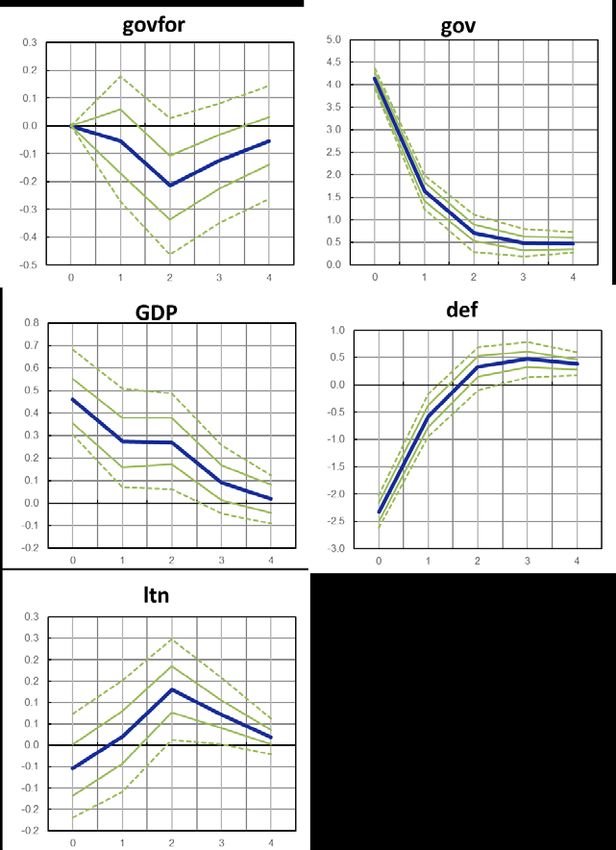
4.1.4 Robustness

 The benchmark results are robust to an alternative model specification and
 other identification assumptions. Table 1 summarises the multipliers estimated in a
 number of alternative models. It is evident that the benchmark results remain robust
 when a different lag structure, a different ordering of variables and a model which
 includes the real effective exchange rate are used. Cumulative spillover multipliers are
 quantitatively close, between 0.3 and 0.4 respectively after two and four years, while
 the time profile of the output reaction varies slightly between these alternative models.

 Table 1
 Robustness of destination spillovers

 Average cumulative multipliers in one euro area country of a trade-weighted €1 increase in
 government spending in the other euro area countries

 Period Benchmark Foreign gov. spending ordered last 1 lag Incl. real effective exchange rate

 0 -0.23 0.00 -0.38 -0.26

 1 0.33 *0.40 0.07 0.30

 2 *0.42 *0.36 0.25 *0.39

 3 0.39 *0.31 *0.32 0.34

 4 0.32 *0.26 *0.35 0.26

 Source: Schmidt (2019).
 Note: * denotes significance at the 68% level.

 Spillovers are somewhat lower when the years following the financial crisis are
 excluded from the estimations. Chart 3 (right panel) shows the (non-cumulative)
 output response to a foreign government spending shock in the estimation for the
 shorter sample from 1972 to 2007, which excludes the period of the Great Recession,
 compared to the full sample estimates (left panel). The output response is comparable
 to the full sample in the first year, but it tends towards zero much faster thereafter
 (impact close to zero from the second year). Cumulative multipliers are therefore only
 slightly smaller than in the full sample after two years (0.25 against 0.42) but
 significantly smaller after four years (0.02 against 0.32). These differences might be
 related to state dependencies in fiscal spillovers that stem from the cyclical position of
 the economy, the reaction of monetary policy and/or the negative fiscal shocks that
 are only observed in the years during and after the financial crisis.

 Spillovers are also lower when limiting the panel to the four largest euro area
 countries (Germany, France, Italy and Spain). For a trade-weighted government
 spending shock in the three largest countries, output in the remaining country
 increases on average by only 0.1 percentage point in the first year (not significant at
 the 68% level) and by 0.2 percentage point in the second year (significant at the 68%
 level) after the shock. However, owing to a stronger negative output response on
 impact, cumulative multipliers are close to zero after two years, increasing only to
 0.15 after four years (against 0.32 in the full panel). The main reason for this smaller
 spillover effect for larger countries should be that they are less open than some of the

 ECB Occasional Paper Series No 240 / April 2020 11

small, open economies included in the main panel set, which, on average, generate
 much larger spillover effects. 9

 Chart 3
 PVAR estimates of government spending (by destination), sample robustness

 Average (non-cumulative) output response in a euro area country to a trade-weighted
 spending increase in the other euro area countries, full sample (left panel) and sample ending
 2007 (right panel)
 (x-axis: years; y-axis: percentage change)

 Source: Schmidt (2019).

4.2 Structural vector autoregression estimates of government
 spending spillovers
 This section provides individual estimates of government spending spillovers
 for the four largest euro area countries using structural vector autoregression
 (SVAR) models. 10 This disaggregated approach allows us to understand the
 potentially heterogeneous effects between countries and gain an insight into the
 transmission mechanisms of fiscal spillovers.

4.2.1 Data

 Estimates are based on a new dataset for euro area countries. An analysis of the
 effects of fiscal spillovers based on time series methods requires the use of
 comparable, long and detailed data. However, for euro area countries, data on many
 of the necessary fiscal variables are only available at a quarterly frequency from the
 mid to late 1990s. This issue is addressed by assembling a new dataset for Germany,
 France, Italy, Spain and the euro area as a whole, from the first quarter of 1980 to the

 9
 The four largest euro area countries have an import-to-GDP ratio (imports from the euro area) of 10%
 over the 1972-2017 period against 26% for the smaller countries in the panel. Other factors such as
 differences in the composition of public spending across countries or a stronger response of interest
 rates to fiscal shocks in large countries might also explain some of the differences.
 10
 For further information on the methodology and results of the estimates presented in this section,
 including the construction of the new quarterly dataset, see Alloza et al. (2019a).

 ECB Occasional Paper Series No 240 / April 2020 12

fourth quarter of 2015 at a quarterly frequency, consistent with Eurostat data (in the
 current ESA 2010 accounting framework). In particular, using an unobserved
 component model that combines both annual and quarterly national accounts, as well
 as monthly indicators, it is possible to estimate fiscal variables at a quarterly
 frequency, while maintaining coherence with official annual aggregates. This
 framework takes into account important features of the data, such as different
 seasonal patterns. 11

 The resulting dataset contains disaggregated measures of fiscal spending (and
 revenues) for each of the four countries and the euro area aggregate. This
 disaggregation allows the separation of components of government spending
 depending on their sensitivity to economic conditions. To support the empirical
 strategy described in the next section, the government spending aggregate comprises
 government consumption and investment, while cyclically sensitive items such as
 transfers are excluded. 12

4.2.2 Methodology

 The empirical strategy follows three steps. First, country-specific VARs are
 estimated based on (the logs of) real net tax revenues, government spending, output,
 the GDP deflator and the level of the 10-year interest rate. The identifying assumption
 is that it takes longer than one quarter to implement fiscal policies in response to a
 change in the economic environment. This facilitates the identification of structural
 shocks to government spending, i.e. fiscal actions are contemporaneously unrelated
 to the economic conditions (see Blanchard and Perotti (2002)). Second, local
 projections are used to trace the dynamic response of economic activity in a country to
 a government spending shock originating in another country (see Jordà (2005)). This
 framework permits the estimation of the bilateral effect of fiscal action for each
 two-country combination. Third, these pair-wise estimates are combined into two
 statistics that summarise the results.

 The dynamic effects of the shocks are estimated using local projections. In
 particular, we estimate the following regressions for output (Y) and government
 spending (G) for each country i:

 , +ℎ − , −1 ℎ , 
 = ,ℎ + , ,ℎ + ,ℎ ( ) , −1 + ξ , +ℎ
 , −1 , −1

 , +ℎ − , −1 ℎ , 
 = ,ℎ + , ,ℎ + ,ℎ ( ) , −1 + , +ℎ
 , −1 , −1

 where ℎ , is a government spending shock in country j identified in a previous
 step, and , −1is a vector of control variables that includes real net tax revenues,

 11
 For Germany and Italy, we combine official information from the quarterly non-financial accounts for
 general government statistics (ESA 2010 and ESA 95) and extend it backwards using intra-annual
 monthly fiscal information and annual official statistics. For Spain and the euro area, we obtain our data
 from updated versions of de Castro et al. (2018) and Paredes et al. (2014) respectively, which were
 constructed according to the methodology described above and are also consistent with national
 accounts. Data for France are obtained directly from Eurostat.
 12
 Nominal variables are converted to real terms using the GDP deflator.

 ECB Occasional Paper Series No 240 / April 2020 13

government spending, output, the GDP deflator and the level of the 10-year interest
 rate in countries i and j. The above equations are estimated for each quarter (h) of the
 response horizon (which extends to 12 periods). The sequence of coefficients , ,ℎ
 for each h of the response horizon represents the dynamic effect of a government
 spending shock in country j on output in country i at period h. These coefficients can
 be combined for various countries, to form spillovers by origin or by destination.

4.2.3 Structural vector autoregression results

 The results provide additional support for the existence of positive fiscal
 spillovers in the euro area. Chart 4 plots the GDP response in each of the four
 economies to increases in government spending in the remaining countries (i.e. the
 destination spillover). The blue line shows the output response in the receiving country
 to the government spending shocks in the source countries, using the coefficients
 , ,ℎ estimated above. Cumulating these output effects and dividing them by the
 cumulated response of government spending ( , ,ℎ ) in the stimulating countries (not
 shown) converts them into a measure that is directly comparable with the multiplier of
 a domestic fiscal expansion. For example, France has a cumulative destination
 spillover of 0.72 after two years. This means that a simultaneous (initial) €1 increase in
 government spending in Germany, Italy and Spain would increase French output by
 €0.72 after two years.

 There are differences in dynamics, magnitude and significance of destination
 spillovers across countries. France and Spain show a similar pattern, with the
 spillover becoming positive and significant at the 68% level by the end of the first year.
 In both cases, the dynamics are similar: around 0.2-0.3 in the first year and
 cumulatively around 0.6-0.7 in the second year. Germany also shows an increasing
 positive spillover, but with significant values at the 68% level, only in the third year.
 While only marginally significant, the magnitude of the effect in Germany seems to be
 larger than in the rest of the countries considered, with a cumulative destination
 spillover of 0.6 at the end of the first year. The spillover in Italy is estimated to be the
 lowest and not significantly different from zero. If the 95% confidence level were
 applied, then fiscal spillovers would only be significant in the case of Spain.

 ECB Occasional Paper Series No 240 / April 2020 14

Chart 4
SVAR estimates of spillover effects (by destination)

Output response to a simultaneous increase in government spending in the rest of the
countries
(x-axis: quarters; y-axis: percentage change)

 Germany France
 1.0 1.0

 0.8 0.8

 0.6 0.6

 0.4 0.4

 0.2 0.2

 0.0 0.0

-0.2 -0.2

-0.4 -0.4
 1 2 3 4 5 6 7 8 9 10 11 12 1 2 3 4 5 6 7 8 9 10 11 12

 Italy Spain
 1.0 1.0

 0.8 0.8

 0.6 0.6

 0.4 0.4

 0.2 0.2

 0.0 0.0

-0.2 -0.2

-0.4 -0.4
 1 2 3 4 5 6 7 8 9 10 11 12 1 2 3 4 5 6 7 8 9 10 11 12

Source: Alloza et al., 2019a.
Note: The blue line shows the output response. The dark grey and light grey lines represent Newey-West confidence intervals at 68%
and 95%.

Positive spillovers are also found for spending increases in one country. When
looking at the spillover effect from the point of view of the country conducting the fiscal
expansion, i.e. spillovers by origin, the results are heterogeneous but also provide
evidence of positive fiscal spillovers among large euro area countries. This effect is
calculated as an output-weighted average of the cross-country spillovers that
country j generates on the rest of countries i ≠ j (the cumulated sum of the ratio of , ,ℎ
to , ,ℎ ). In particular, government spending spillovers by origin are estimated to be
stronger in Italy and Spain than in Germany, but not significant for France (Chart 5).
Additionally, spillovers by origin are found to be stronger for public investment than
consumption.

ECB Occasional Paper Series No 240 / April 2020 15

Chart 5
 SVAR estimates of spillover effects (by origin)

 Output response to an increase in government spending in one country in the other euro area
 countries
 (x-axis: quarters; y-axis: percentage change)

 Source: Alloza et al., 2019a.
 Note: The blue line shows the output response. The dark grey and light grey lines represent Newey-West confidence intervals at 68%
 and 95%.

4.2.4 Potential sources of country heterogeneity

 Differences in trade intensity between countries are likely to be an important
 driver of transmissions of fiscal stimuli. An increase in government spending in a
 country raises both the domestic aggregate demand and the imports from a different
 country. A pair of countries with a tight trade relationship is likely to experience larger
 fiscal spillovers. 13

 13
 Alloza, et al. (2019a) show that there is a substantial and positive relationship between the size of
 cross-country government spending spillovers and their corresponding share of bilateral imports.

 ECB Occasional Paper Series No 240 / April 2020 16

Chart 6
 Response of euro area-wide interest rate to (domestic) government spending shock

 Euro area-wide interest rate response to an increase in government spending in one country
 (x-axis: quarters; y-axis: percentage change)

 Germany France
 0.4 0.4

 0.3 0.3

 0.2 0.2

 0.1 0.1

 0.0 0.0

 -0.1 -0.1

 -0.2 -0.2
 1 2 3 4 5 6 7 8 9 10 11 12 1 2 3 4 5 6 7 8 9 10 11 12

 Italy Spain
 0.4 0.4

 0.3 0.3

 0.2 0.2

 0.1 0.1

 0.0 0.0

 -0.1 -0.1

 -0.2 -0.2
 1 2 3 4 5 6 7 8 9 10 11 12 1 2 3 4 5 6 7 8 9 10 11 12

 Source: Alloza et al., 2019a.
 Note: The blue line shows the interest rate response. The dark grey and light grey lines represent Newey-West confidence intervals at
 68% and 95%.

4.2.5 Comparison of PVAR and SVAR results

 The results from the PVAR and SVAR estimates broadly show a similar picture.
 The abovementioned SVAR destination spillovers measure the impact of a
 €1 increase in government spending in each of the other euro area countries. 14 An
 alternative measure is the effect of an average €1 spending increase in the other three
 euro area countries, which results in lower spillovers on the remaining country but with
 a similar heterogeneity across countries (see Table 2). For the four largest euro area
 countries, the output-weighted average spillovers are around 0.09, 0.46 and 0.60 in
 the first, second and third years respectively. These figures are broadly comparable to
 the results of the PVAR estimates described in Section 2.1, which are based on
 annual data for 11 euro area countries: 0.33, 0.42 and 0.39. The similarity between

 14
 Since this spillover is based on adding the estimated effects of fiscal shocks that might not have taken
 place at the same moment in time, the results are likely to represent an upper bound.

 ECB Occasional Paper Series No 240 / April 2020 17

both sets of results is confirmed with PVAR multipliers estimated on a sample with the
same starting year as the SVAR estimates (0.22, 0.38 and 0.43). The differences
become somewhat larger when compared with the PVAR estimates, which include
only the four largest euro area countries, and show smaller spillover effects (0.02 after
two years, 0.23 after three years). 15 When comparing the benchmark results, both
analyses suggest that the average destination spillover during the first two years is
close to 0.4.

Table 2
Comparison of destination spillovers

Cumulative multiplier (two-year)

 Method SVAR PVAR

 Countries DE FR IT ES EA# EA DE, FR, IT, ES

 Sample 1980Q1-2016Q4 1972-2017 1980-2017 1980-2017

 Average destination spillover 0.73 **0.50 0.00 **0.32 0.46 *0.42 *0.38 0.02

 Simultaneous destination spillover 1.72 *0.72 0.16 *0.61

Source: Alloza et al. (2019) and Schmidt (2019).
Notes: Average destination spillover measures the output response to a €1 average government spending increase in the other euro
 #
area countries; simultaneous spillovers measure the output response to a €1 increase in each of the other countries. EA average based
on the output-weighted average of the SVAR results; * denotes significance at the 68% level; ** at the 95% level.

The results are broadly comparable with previous empirical studies. Different
data samples, fiscal identification and estimation methods make a comparison with
other papers somewhat complicated. However, our baseline results are close to
PVAR estimates found by Beetsma and Giuliodori (2011) and Dabla-Norris et al.
(2017). Their magnitude is at the lower end of estimates by Auerbach and
Gorodnichenko (2013) and Blagrave et al. (2017). 16

The effect of fiscal spillovers is smaller than domestic fiscal spending. The
domestic multipliers found in both approaches are very similar. The second-year
cumulative multiplier for the euro area is 1.1 in the SVAR, with estimates for individual
countries varying between 1.1 and 1.4 (Alloza et al. (2019a)). The PVAR estimate is
0.9 (see Section 3.1.3). These results suggest that the spillover effect of fiscal
expenditure across euro area countries is below half of the effect of domestic fiscal
expenditure.

15
 However, there is a higher degree of uncertainty surrounding the PVAR estimates for the sample
 restricted to the four largest euro area countries, and the spillover multipliers are not significant (at the
 68% level).
16
 The average three-year spillover multipliers reported in these papers differ between 1.4 and 2.0,
 depending on the identification of fiscal shocks and estimation methods (see Annex 6 in Blagrave et al.
 (2017)). The difference in results may be due to differences in the data used (shorter time samples and
 covering OECD countries). The reported uncertainty bands do not allow us to conclude that our results
 are significantly lower.

ECB Occasional Paper Series No 240 / April 2020 18

5 Spillover analysis based on a
 multi-country DSGE model

 This section provides simulations using a multi-country DSGE model: the Euro
 Area and Global Economy (EAGLE) model. 17 The model is calibrated with the euro
 area split into five blocs – Germany, France, Italy, Spain and the rest of the euro
 area – while the sixth bloc covers the rest of the world. 18 Like the ECB’s New
 Area-Wide Model, EAGLE is micro-founded and features nominal price and wage
 rigidities, capital accumulation, and international trade in goods and bonds. Given its
 global dimension, the model is particularly well suited to assess cross-border
 spillovers. All regions trade with each other in intermediate goods, with estimates of
 bilateral trade flows based on recent historical averages. International asset trade is
 limited to nominally non-contingent bonds denominated in US dollars.

 The version used here embeds an extended fiscal bloc. 19 Households are
 assumed to derive utility from the consumption of a composite good consisting of
 public and private consumption goods. Following Clancy et al. (2016) and Coenen et
 al. (2012), government consumption CG,t enters as a partial complement to private
 consumption Ct in the utility function. Utility depends on aggregated consumption CCt:

 θ
 1 θ−1 1 θ−1 θ−1
 CCt = �ωθ (Ct ) θ + (1 − ω)θ �CG,t � θ � (1)

 The share of the government consumption good in the composite good is determined
 by ω, while θ determines the degree of complementarity. Therefore, changes in
 government consumption directly affect optimal private consumption decisions, as
 opposed to the indirect wealth effect when government consumption is separable (see
 Clancy et al. (2016)).

 It is also assumed that government capital stock affects the production process. The
 model also explicitly accounts for the fact that government investment, IG,t is assumed
 not to be wasteful and contributes to public capital, KG,t as in Leeper et al. (2010):

 K G,t+1 = (1 − δ)K G,t+1 + IG,t (2)

 where δ is the depreciation rate. In each sector, KG,t enters the production function as
 follows:

 Yt = zt K εG,t Kαt L1−α
 t (3)

 17
 The model simulations in this chapter were previously published in Alloza et al. (2019b).
 18
 The Euro Area and Global Economy (EAGLE) model is a multi-country dynamic stochastic general
 equilibrium model of the euro area developed by an ESCB team composed of staff from the Banca
 d’Italia, the Banco de Portugal and the ECB. See Gomes et al. (2012).
 19
 See Clancy et al. (2016).

 ECB Occasional Paper Series No 240 / April 2020 19

where zt is the exogenous technological progress, Kt the private capital and Lt labour
(with share α and 1-α respectively). Government capital enhances the productivity of
private capital in a similar manner to technological progress (with productivity ε). This
implies that an increase in government capital will reduce the marginal costs, MCt, of
the intermediate goods sector:

 −1 α 1−α
MCt = �zt K ϵG,t αα (1 − α)1−α � �RK,t � �Wt �1 + τL,t �� (4)

Moreover, in each country, public debt (Bt) is stabilised through a fiscal rule that
induces the endogenous adjustment of fiscal instruments when the public debt ratio
deviates from its target (BY).

 Bt
τt = φB � − BY� (5)
 Pt Yt

Members of the euro area share a common nominal exchange rate and a
common nominal interest rate. The central bank sets the domestic short-term
nominal interest rate (it) according to a standard Taylor-type rule, by reacting to
area-wide consumer price inflation and real activity.

 Yt
it = ρ it−1 + (1 − ρ) φπ (πt − π∗ ) + φY � − 1� (6)
 Yt−1

The rest of the world has its own nominal interest rate and nominal exchange rate.
When forward guidance is implemented, the given monetary policy authority
announces that nominal interest rates will be fixed for a certain time period.

The calibration of parameters that determine the aggregation of private and
government consumption expenditure follows Coenen et al. (2012). The elasticity of
substitution between private and government consumption (θ) is set to 0.30, and the
quasi-share of government consumption expenditure in the aggregator (1- ω) is equal
to 0.20. This ensures that the observed responses of consumption to government
spending shocks are in line with either country-specific or euro area evidence
(e.g. Kirchner et al. (2010); Coenen et al.(2012)). As such, government and private
consumption are strong, but not perfect, complements, in line with the evidence in
Karras (1994) and Fiorito and Kollintzas (2004). On the supply side, the bias towards
public (ε) capital in the production function of intermediate goods sectors is equal to
0.10.

The coefficients of the fiscal rule and the monetary policy rule use standard values
from the literature and are in line with the New Area-Wide Model (Christoffel et al.
(2008)) and the original EAGLE (Gomes et al. (2012)). The coefficient in the fiscal rule
(φB) is equal to 0.1. For the monetary policy rule, the steady-state level of inflation (π*)
is equal to the inflation target, set to 2%, while parameters of the rule take the values ρ,
φπ and φY equal to 0.87, 1.70, and 0.10 respectively.

The simulations focus on government consumption and public investment
separately. The following two sections show the spillovers of a two-year

ECB Occasional Paper Series No 240 / April 2020 20

spending-based fiscal stimulus, which is debt-financed, for two alternative
 specifications: first, with interest rates set according to the Taylor rule; second, with
 unchanged interest rates. The results are shown for government consumption and
 public investment separately.

5.1 Spillovers with reactive and non-reactive monetary policy
 When interest rates respond to the fiscal shock, spillovers by origin are
 positive but small. The left-hand panel in Chart 7 shows the spillovers from a fiscal
 stimulus of 1% of nominal GDP over two years in one large euro area country to the
 rest of the euro area, both for government investment and for consumption. 20 While
 there is some cross-country heterogeneity, both in the domestic effect (shown on the
 x-axis) and the effect on the other countries (y-axis), the spillovers (computed as the
 ratio of the GDP reaction of destination to source) are below 0.1 on average in the two
 years after the shock.

 Chart 7
 Model simulations of fiscal spillovers (with reactive interest rates)
 (x-axis: two-year average percentage change in GDP in country(-ies) propagating the fiscal stimulus; y- axis: two-year average
 percentage change in GDP in recipient country)

 DE (government consumption) IT (government consumption)
 DE (public investment) IT (public investment)
 FR (government consumption) ES (government consumption)
 FR (public investment) ES (public investment)

 a) Spillovers by origin b) Spillovers by destination
 0.2 0.2

 0.1 0.1

 0.0 0.0

 -0.1 -0.1
 0.0 0.5 1.0 1.5 2.0 0.0 0.5 1.0 1.5 2.0

 Source: EAGLE model.
 Notes: The left-hand panel shows the spillover by origin, i.e. the impact of an increase in government consumption or public investment
 by 1% of GDP for two years in one country on its own output (x-axis) and the output of the other countries (y-axis). The right-hand panel
 shows the spillover by destination, i.e. the impact of a simultaneous increase in government consumption or public investment by 1% of
 GDP for two years in all but one country on the countries’ output (x-axis) and the country receiving the spillovers (y-axis).

 Spillovers by destination are also small. The right-hand panel in Chart 7 shows the
 spillovers in one large country from a simultaneous fiscal stimulus of 1% of GDP over
 two years in the other countries. For public investment, the spillovers come out at just
 above 0.1. For public consumption, the destination spillovers are on average slightly
 negative during the first two years, mainly because the demand effect of the fiscal
 stimulus is offset by the contractionary impact of higher interest rates that applies to all
 countries in the monetary union. Relative country size is also important: the
 20
 In this and the following model simulations, the size of the stimulus (1% of GDP of the country or
 countries conducting the stimulus) is chosen for convenience in the interpretation of the results.

 ECB Occasional Paper Series No 240 / April 2020 21

destination spillover in Spain is somewhat larger than the destination spillover in
Germany. This is because the former results from a 1% of GDP stimulus in all
countries but Spain and the latter from a 1% of GDP fiscal expansion in all countries
but Germany.

Destination spillovers are not identical to an aggregation of the spillovers by
origin. Both the spillovers and the domestic effect on output in the countries
conducting the stimulus are more clustered. One explanation is that the impact of a
simultaneous stimulus on prices and economic activity is larger and triggers a
relatively stronger monetary reaction than a stimulus in one large euro area country.

When interest rates in the euro area do not respond to the fiscal shock,
spillovers by origin and by destination are positive, and much larger than in the
case of reactive monetary policy. Without a reaction from interest rates for two
years, spillovers by origin vary between 0.07 for an increase in government
consumption in Spain by 1% of GDP and 0.25 for a similar increase in German public
investment (see the left-hand panel in Chart 8). These spillovers are around six times
as large as those with responsive interest rates. A similarly strong increase can be
seen for investment-based spillovers by destination (see the right-hand panel in
Chart 8). The sensitivity of destination spillovers to France, Italy and Spain to the
reaction of interest rates is even stronger for a public consumption-based stimulus,
with the effect increasing from a negative value to above 1. 21

The model simulations largely confirm the empirical estimates presented
above. When interest rates react, spillovers are generally positive but small, and
higher for investment than for consumption. When comparing the model simulations
with the empirical estimates of the destination spillovers, it should be taken into
account that the empirical estimates are based on data covering different monetary
policy regimes and without coordinated fiscal policies (except in the 2009-10 period of
the crisis). The relatively high empirical destination spillovers for Germany might
partially reflect the fact that fiscal stimulus episodes in the other large euro area
countries resulted less often in an increase in interest rates, on account of exchange
rate pegs to the Deutsche Mark prior to EMU, or their smaller weight in the euro area
economy since the introduction of a common monetary policy.

21
 The exercise is restricted to fiscal shocks and does not take into account other shocks that would have
 led to forward guidance, such as depressed private demand and credit-constrained households and firms
 following an economic crisis. From a longer-term perspective, an increase in public investment could
 generally be expected to contribute more to the productive capacity of the economy than government
 consumption. Non-standard monetary policy measures that can lessen the constraints of the effective
 lower bound are also not considered in this analysis.

ECB Occasional Paper Series No 240 / April 2020 22

Chart 8
 Model simulations of fiscal spillovers (with reactive interest rates)
 (x-axis: two-year average percentage change in GDP in country(-ies) propagating the fiscal stimulus; y- axis: two-year average
 percentage change in GDP in recipient country)

 DE (government consumption) IT (government consumption)
 DE (public investment) IT (public investment)
 FR (government consumption) ES (government consumption)
 FR (public investment) ES (public investment)

 a) Spillovers by origin b) Spillovers by destination
 0.3 1.4

 1.2

 1.0
 0.2

 0.8

 0.6
 0.1
 0.4

 0.2

 0.0 0.0
 0.0 0.5 1.0 1.5 2.0 0.0 0.5 1.0 1.5 2.0 2.5

 Source: EAGLE model.
 Notes: The left-hand panel shows the spillover by origin, i.e. the impact of an increase in government consumption or public investment
 by 1% of GDP for two years in one country on its own output (x-axis) and the output of the other countries (y-axis). The right-hand panel
 shows the spillover by destination, i.e. the impact of a simultaneous increase in government consumption or public investment by 1% of
 GDP for two years in all but one country on the countries’ output (x-axis) and the country receiving the spillovers (y-axis).

5.2 Sensitivity analysis
 Structural models are sensitive to the assumptions regarding future
 developments in monetary policy. The simulations above are conducted under the
 assumptions of perfect foresight and complete financial markets. The implication of
 these assumptions is that the monetary authority, firms and households all know of
 and are able to completely adjust to future changes in the monetary and fiscal policy
 stances. Through these features, structural models are known to be very sensitive to
 the announcement of future interest rates, which is known in the theoretical literature
 as the “forward guidance puzzle”. 22

 As indicated by McKay et al. (2016): “Standard monetary models imply that far future
 forward guidance is extremely powerful: promises about far future interest rates have
 huge effects on current economic outcomes, and these effects grow with the horizon
 of the forward guidance.” The solution to the forward guidance puzzle is either making
 the model less forward-looking or altering expectations (e.g. so that the
 announcement is not partially misperceived). As an illustrative example, let us
 consider the standard IS curve:

 xt = Et xt+1 − σ�it − Et πt+1 − rn,t � (7)

 where xt is the output gap, i t is the nominal interest rate, πt is CPI inflation and rn,t is the
 real natural rate of interest. When the equation is intertemporally solved, it implies:

 22
 See McKay et al. (2016) or Del Negro et al. (2015).

 ECB Occasional Paper Series No 240 / April 2020 23

∞
xt = −σ � Et �it+j − Et+j πt+j+1 − rn,t+j � (8)
 j=0

We can see that there is no discounting in the sum on the right-hand side of this
equation. This means that after a stimulating monetary policy shock, the output gap
will increase immediately and will stay at that higher level until the low interest rate
period passes. One possibility to smooth out this strong effect would be discounting
the equation by a β parameter:

xt = β Et xt+1 − σ�it − Et πt+1 − rn,t � (9)

This would mean that after resolution, the equation becomes:

 ∞
xt = −σ � Et βj �it+j − Et+j πt+j+1 − rn,t+j � (10)
 j=0

In this way, the forward guidance puzzle is mitigated. Close to the value proposed by
McKay et al. (2016), β is calibrated to 0.98. An alternative strategy entails considering
that economic agents might be myopic, thus revising their perception of the monetary
policy on a regular basis (e.g. annually). In order to obtain realistic results, the model
has been adjusted to take the forward guidance puzzle into account. The two types of
adjustments were implemented in our simulation exercises.

Spillovers are also affected by the forward guidance puzzle. The sensitivity to
future interest rates does not only apply to the domestic effect of a fiscal stimulus but
also to the spillover ratio – the ratio of the average percentage change in GDP in the
recipient country to the percentage change in GDP in the stimulating country. An
illustration for a public investment-based stimulus in Germany shows that the spillover
ratio increases more than proportionally when the announced path of future interest
rates is extended by one year (see Chart 9). The effect becomes much smaller when
the interest rate path is modelled as a series of one-year announcements (bars
labelled “myopic”) or when households and firms in the model discount the future
impact of the expected real interest rate on current consumption and investment
decisions (bars labelled “disc.”). 23 This sensitivity analysis suggests that the size of
spillovers under an expected path of unchanged interest rates are sensitive to the
specification of the monetary policy rule, which should avoid the results being driven
by the forward guidance puzzle. The simulations shown in Section 3.1 are modelled
with the stable interest rate path as a series of one-year announcements.

23
 See McKay et al. (2017).

ECB Occasional Paper Series No 240 / April 2020 24