The Effects of Monetary Policy on Stock Market Bubbles: Some Evidence
←
→
Page content transcription
If your browser does not render page correctly, please read the page content below
The E¤ects of Monetary Policy on Stock Market Bubbles:
                                      Some Evidence
                               Jordi Galiy            Luca Gambettiz

                                          December 2013

                                              Abstract

          We estimate the response of stock prices to exogenous monetary policy shocks using
      a vector-autoregressive model with time-varying parameters. Our evidence points to
      protracted episodes in which, after a a short-run decline, stock prices increase per-
      sistently in response to an exogenous tightening of monetary policy. That response
      is clearly at odds with the "conventional" view on the e¤ects of monetary policy on
      bubbles, as well as with the predictions of bubbleless models. We also argue that it is
      unlikely that such evidence be accounted for by an endogenous response of the equity
      premium to the monetary policy shocks.

         JEL Classi…cation: E52, G12
         Keywords: leaning against the wind policies, …nancial stability, in‡ation targeting,
      asset price booms.

     We have bene…ted from comments by Andrea Ferrero, Mark Gertler Refet Gürkeynak, Lucrezia Rieichlin,
and seminar and conference participants at UB, CEMFI, NYU, the Barcelona GSE Summer Forum, the Time
Series Econometric Workshop (U. Zaragoza), the Norges Bank Conference on "The Role of Monetary Policy
Revisited", the NBER Conference on "Lessons for the Financial Crisis from Monetary Policy" and the
OFCE Workshop on Empirical Monetary Economics. Galí acknowledges the European Research Council for
…nancial support under the European Union’s Seventh Framework Programme (FP7/2007-2013, ERC Grant
agreement no 339656). Gambetti gratefully acknowledges the …nancial support of the Spanish Ministry of
Economy and Competitiveness through grant ECO2012-32392 and the Barcelona GSE Research Network.
   y
     CREI, UPF and Barcelona GSE. E-mail: jgali@crei.cat
   z
     UAB and Barcelona GSE. E-mail: luca.gambetti@uab.edu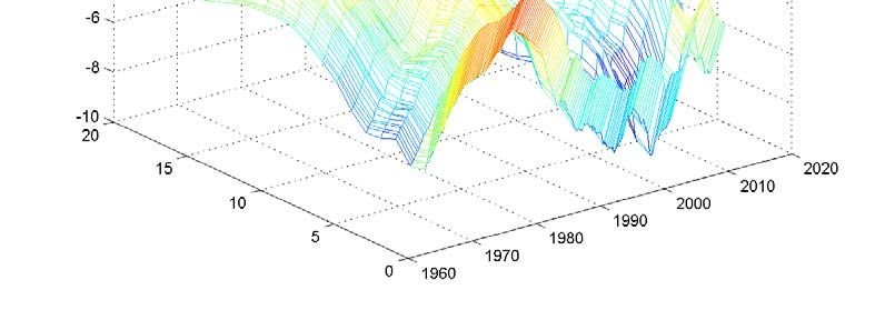
The economic and …nancial crisis of 2008-2009 has been associated in many countries
with a rapid decline in housing prices, following a protracted real estate boom. This has
generated a renewed interest in the link between monetary policy and asset price bubbles,
and revived the long standing debate on whether and how monetary policy should respond
to perceived deviations of asset prices from fundamentals.1
    The consensus view before the crisis was that central banks should focus on stabilizing
in‡ation and the output gap, and ignore ‡uctuations in asset prices, even if the latter are
perceived to be driven by bubbles.2 The recent crisis has challenged that consensus and has
strengthened the viewpoint that central banks should pay attention and eventually respond
to developments in asset markets. Supporters of this view argue that monetary authorities
should "lean against the wind," i.e. raise the interest rate to counteract any bubble-driven
episode of asset price in‡ation, even at the cost of temporarily deviating from their in‡ation
or output gap targets. Any losses associated with these deviations, it is argued, would be
more than o¤set by the avoidance of the consequences of a future burst of the bubble.3
    A central tenet of the case for "leaning against the wind" monetary policies is the
presumption that an increase in interest rates will reduce the size of an asset price bubble.
While that presumption may have become part of the received wisdom, no empirical or
theoretical support seems to have been provided by its advocates.
    In recent work (Galí (2014)), one of us has challenged, on theoretical grounds, the link
between interest rates and asset price bubbles underlying the conventional view. The reason
is that, at least in the case of rational asset price bubbles, the bubble component must grow,
in equilibrium, at the rate of interest. If that is the case, an interest rate increase may end
up enhancing the size of the bubble. Furthermore, and as discussed below, the theory of
rational bubbles implies that the e¤ects of monetary policy on observed asset prices should
depend on the relative size of the bubble component. More speci…cally, an increase in the
interest rate should have a negative impact on the price of an asset in periods where the
bubble component is small compared to the fundamental. The reason is that an interest
rate increase always reduces the ”fundamental” price of the asset, an e¤ect that should be
dominant in "normal" times, when the bubble component is small or non existent. But
if the relative size of the bubble is large, an interest rate hike may end up increasing the
   1
     Throughout the paper we use the term "monetary policy" in the narrow sense of "interest rate policy."
Thus we exclude from that de…nition policies involving macroprudential instruments which are sometimes
controlled by central banks and which may also be used to stabilize asset prices.
   2
     See, e.g. Bernanke and Gertler (1999, 2000) and Kohn (2006). Two arguments have been often pointed
to in support of that view: (i) asset price bubbles are di¢ cult to detect and measure, and (ii) interest rates
are "too blunt" an instrument to prick a bubble, and their use with that purpose may have unintended
collateral damages.
   3
     See, e.g., Borio and Lowe (2002) and Cecchetti et al. (2000) for an early defense of "leaning against the
wind" policies.

                                                      1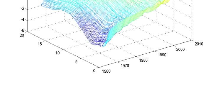
observed asset price over time, due to its positive e¤ect on the bubble more than o¤setting
the negative impact on the fundamental component.
     In the present paper we provide evidence on the dynamic response of stock prices to
monetary policy shocks, and try to use that evidence to infer the nature of the impact of
interest rate changes on the (possible) bubble component of stock prices..Our main goal
is to assess the empirical merits of the "conventional" view. Under the latter, the size of
the bubble component of stock prices should decline in response to an exogenous increase
in interest rates. Since the fundamental component is expected to go down in response to
the same policy intervention, any evidence pointing to a positive response of observed stock
prices (i.e. of the sum of the fundamental and bubble components) to an exogenous interest
rate hike would call into question the conventional view regarding the e¤ects of monetary
policy on stock price bubbles.
     Our starting point is an estimated vector-autoregression (VAR) on quarterly US data
for GDP, the GDP de‡ator, a commodity price index, dividends, the federal funds rate, and
a stock price index (S&P500). Our identi…cation of monetary policy shocks is based on the
approach of Christiano Eichenbaum and Evans (2005; henceforth, CEE), though our focus
here is on the dynamic response of stock prices to an exogenous hike in the interest rate.
Also, and in contrast with CEE, we allow for time-variation in the VAR coe¢ cients, which
results in estimates of time-varying impulse responses of stock prices to policy shocks.4 In
addition to the usual motivations for doing this (e.g. , structural change), we point to a
new one which is speci…c to the issue at hand: to the extent that changes in interest rates
have a di¤erent impact on the fundamental and bubble components, the overall e¤ect on
the observed stock price may change over time as the relative size of the bubble changes.
     Under our baseline speci…cation, which assumes no contemporaneous response of mone-
tary policy to asset prices, the evidence points to protracted episodes in which stock prices
increase persistently in response to an exogenous tightening of monetary policy. That re-
sponse is clearly at odds with the "conventional" view on the e¤ects of monetary policy on
bubbles, as well as with the predictions of bubbleless models.
     We assess a variety of alternative explanations for our …ndings. Thus, we argue that
it is unlikely that such evidence be accounted for by an endogenous response of the equity
premium to the monetary policy shocks.
     When we allow for an endogenous contemporaneous response of interest rates to stock
prices, and calibrate the relevant coe¢ cient in the monetary policy rule according to the
…ndings in Rigobon and Sack (2003), our …ndings change dramatically: stock prices decline
substantially in response to a tightening of monetary policy, more so than our estimated
  4
   See, e.g. Primiceri (2005) and Gali and Gambetti (2009) for some macro applications of the TVC-VAR
methodology.

                                                 2
fundamental components. That …nding would seem to vindicate the conventional view on
the e¤ectiveness of leaning against the wind policies. Recent evidence by Furlanetto (2011),
however, calls into question the relevance of this alternative speci…cation for much of the
sample period analyzed, while supporting instead our baseline speci…cation.
Ultimately, our objective is to produce evidence that can improve our understanding of
the impact of monetary policy on asset prices and asset price bubbles. That understanding is
a necessary condition before one starts thinking about how monetary policy should respond
to asset prices.
The remainder of the paper is organized as follows. In Section 1 we discuss alternative
hypothesis on the link between interest rates and asset prices. Section 2 describes our
empirical model. In Section 3 we report the main …ndings under our baseline speci…cation.
Section 4 provides alternative interpretations as well as evidence based on an alternative
speci…cation. Section 5 concludes.
1 Monetary policy and asset price bubbles: Theoretical is-
sues
We use a simple partial equilibrium asset pricing model to introduce some key concepts and
notation used extensively below.5 We assume an economy with risk neutral investors and
an exogenous, time-varying (gross) riskless real interest rate Rt .6 Let Qt denote the price
in period t of an in…nite-lived asset, yielding a dividend stream fDt g.
We interpret that price as the sum of two components: a "fundamental" component,
Qt , and a "bubble" component, QB
F
t . Formally,
Qt = QFt + QB
t (1)
where the fundamental component is de…ned as the present discounted value of future
dividends: (1 ! )
X kQ1
QFt Et (1=Rt+j ) Dt+k (2)
k=1 j=0
or, rewriting it in log-linear form (and using lower case letters to denote the logs of the
original variables)7
1
X
qtF = const + k
[(1 )Et fdt+k+1 g Et frt+k g] (3)
k=0
5
See Galí (2014) for a related analysis in general equilibrium.
6
Below we discuss the implications of allowing for a risk premium.
7
See, e.g., Cochrane (2001, p.395) for a derivation.
3where =R < 1, with and R are denoting, respectively, the (gross) rates of dividend
growth and interest along a balanced growth path.
How does a change in interest rates a¤ect the price of an asset that contains a bubble?
We can seek an answer to that question by combining the dynamic responses of the two
components of the asset price to an exogenous shock in the policy rate. Letting that shock
be denoted by "m
t , we have:
F
@qt+k B
@qt+k
@qt+k
= (1 t 1) + t 1 (4)
@"m
t @"m
t @"m
t
where t QB t =Qt denotes the share of the bubble in the observed price in period t.
Using (2), we can derive the predicted response of the fundamental component
F 1
X
@qt+k j @dt+k+j+1 @rt+k+j
= (1 ) (5)
@"m
t @"m
t @"mt
j=0
Both conventional wisdom and economic theory (as well as the empirical evidence dis-
cussed below) point to a rise in the real interest rate and a decline in dividends in response
to an exogenous tightening of monetary policy, i.e. @rt+k =@"m t > 0 and @dt+k =@"t
m 0 for
k = 0; 1; 2; :::Accordingly, the fundamental component of asset prices is expected to decline
F =@"m < 0 for k = 0; 1; 2; :::
in response to such a shock, i.e. we expect @qt+k t
Under the "conventional view" on the e¤ects of monetary policy on asset price bubbles
we have, in addition:
B
@qt+k
0 (6)
@"m
t
for k = 0; 1; 2; :::i.e. a tightening of monetary policy should cause a decline in the size of
the bubble. Hence, the overall e¤ect on the observed asset price should be unambiguously
negative, independently of the relative size of the bubble:
@qt+kUsing (1), (7) and (8), it can be easily checked that the bubble component must satisfy:8
QB B
t Rt = Et fQt+1 g (9)
or, equivalently, in its log-linear version:
B
Et f qt+1 g = rt
Hence, an increase in the interest rate will raise the expected growth of the bubble
component. Note that the latter corresponds to the bubble’s expected return, which–under
the risk neutrality assumption made here–must be equal to the interest rate. Accordingly,
and as discussed in Galí (2014), any rule that implies a systematic positive response of the
interest rate to the size of the bubble, will tend to amplify the movements in the latter
–an outcome that calls into question the conventional wisdom about the relation between
interest rates and bubbles.
Changes in interest rates, however, may also a¤ect the bubble through a second channel:
a possible systematic comovement between the (indeterminate) innovation in the bubble
with the surprise component of the interest rate. To see this, evaluate the previous expres-
sion at t 1 and eliminate the expectational operator to obtain:
qtB = rt 1 + t (10)
where t qtB Et 1 fqtB g is an arbitrary process satisfying Et 1 f t g = 0 for all t (i.e. the
martingale-di¤erence property). Note that the unanticipated change ("innovation") in the
size of the bubble, t , may or may not be related to fundamentals and, in particular, to
the interest rate innovation, rt Et 1 frt g. Thus, and with little loss of generality, one can
write:
t = t (rt Et 1 frt g) + t (11)
where t is a (possibly random) parameter and f t g is a zero-mean martingale-di¤erence
process, respectively satisfying the orthogonality conditions . Et 1 f t (rt Et 1 frt g)g = 0
and Et 1 f t t (rt Et 1 frt g)g = 0. Note that neither the sign nor the size of t , nor its
possible dependence on the policy regime, are pinned down by the theory. Accordingly,
the contemporaneous impact of an interest rate innovation on the bubble is, in principle,
indeterminate.
The dynamic response of the bubble component to a monetary policy tightening is given
by (
B @rt
@qt+k t @"m for k = 0
m = @r
t
P k 1 @r (12)
@"t t @"m +
t
j=0 @"m
t+j
for k = 1; 2; :::
t t
8
Transversality conditions generally implied by optimizing behavior of in…nite-lived agents are often used
to rule out such a bubble component (see, e.g., Santos and Woodford (1997)). That constraint does not apply
to economies with overlapping generations of …nitely-lived agents (e.g., Samuelson (1958), Tirole (1985)).
5for k = 0; 1; 2; :::.Thus, and as discussed above, the initial impact on the bubble, captured by
coe¢ cient t , is indeterminate, both in sign and size. Yet, and conditional on @rt+k =@"m t >
0, for k = 0; 1; 2; :: the subsequent growth of the bubble is predicted to be positive. The
long run impact of the monetary policy shock on the size of the bubble, limk!1 @qt+k B =@"m
t
will be positive or negative depending on whether the persistence of the real interest rate
response is more than su¢ cient to o¤set any eventual negative initial impact. Thus, when
considered in combination with the predicted response of the fundamental component, the
theory of rational bubbles implies that the sign of the response of observed asset prices
to a tightening of monetary policy is ambiguous. Most importantly, however, the theory
opens the door to the possibility that the observed asset price rises (possibly after some
initial decline), as long as one or more of the following conditions are satis…ed: (i) t is not
"too negative", (ii) the response of the real interest rate is persistent enough, and (iii) the
relative size of the bubble t is large enough (so that the eventual positive response of the
latter more than o¤sets the likely decline in the fundamental component).
To illustrate the previous discussion, consider an asset whose dividends are exogenous
and independent of monetary policy. In response to an exogenous policy tightening the
real interest rate is assumed to evolve according to @rt+k =@"m k
t = r , for k = 0; 1; 2; :::The
response of the (log) asset price to a unit shock is then given by:
@qt+k k 1 k
r r
= (1 t 1) + t 1 t +
@"m
t 1 r 1 r
Figure 1 displays the dynamic responses of the asset price for alternative con…gurations
of and . In all cases we assume = 0:99 and r = 0:8. The black line (with circles)
displays the asset price response in the absence of a bubble ( t 1 = 0). The asset price
declines on impact, and gradually returns to its original value. The blue line (with circles)
shows the response for t = 0:5 and t = 0. Note that the asset price also declines on
impact, but now it recovers at a faster pace (due to the growing bubble) and ends up
overshooting permanently its initial value and stabilizing at a higher level. The red line
(with squares) corresponds to the case of t = 0:5 and t = 8. Now the negative impact
of the interest rate hike on the asset price is larger, due to its initial shrinking e¤ect on the
size of the bubble. Finally, the green line (with triangles) shows the response under t = 0:5
and t = 6. Now the asset price already rises from the time of the shock, given that the
positive response of the bubble on impact more than o¤sets the decline of the fundamental
component.
The previous simulations make clear that the theory of rational bubbles is consistent
with a broad range of responses of asset prices to a tightening of monetary policy. By
contrast, the conventional view predicts an unambiguous decline in asset prices, for both
the fundamental and bubble components are expected to go down in response to a policy
6tightening. Accordingly, any evidence of a decline in asset prices in response to that tight-
ening would not be conclusive as to the validity of the two views on the e¤ects of monetary
policy on the bubble. On the other hand, any evidence of a positive impact on the asset
price at some horizon subsequent to the same policy intervention would be clearly at odds
with both the key premise and the implications of the "conventional view," while consistent
(at least, qualitatively) with the theory of rational bubbles.
2 The empirical model
The present section describes our empirical model, which consists of a structural vector
autoregression model with time-varying coe¢ cients (TVC-SVAR). Beyond the usual concern
for possible structural changes over the sample period considered, our main motivation for
using a model with time-varying coe¢ cients has to do with the dependence of the stock
price response on the relative size of its (eventual) bubble component, which is likely to
change over time.
Though focusing on di¤erent variables, the speci…cation of our reduced form time-
varying VAR follows closely that in Primiceri (2005). On the other hand our choice of
variables and identi…cation strategy follows that in Christiano et al. (2005). Our constant
coe¢ cients VAR, for which we also report results below, can be seen as a limiting case of
the model with time-varying coe¢ cients, so we do not provide a separate description.
Let yt , pt , pct , it , qt , and dt denote, respectively, (log) output, the (log) price level,
the (log) commodity price index, the short-term nominal interest rate controlled by the
central bank, the (log) stock price index, and its corresponding (log) dividend series (both
in real terms). We de…ne xt [ yt ; dt ; pt ; pct , it ; qt ]0 . The relationship between those
variables and the structural shocks is assumed to take the form of an autoregressive model
with time-varying coe¢ cients:
xt = A0;t + A1;t xt 1 + A2;t xt 2 + ::: + Ap;t xt p + ut (13)
where A0;t is a vector of time-varying intercepts, and Ai;t , for i = 1; :::; are matrices of
time-varying coe¢ cients, and where the vector of reduced form innovations ut follows a
white noise Gaussian process with mean zero and covariance matrix t . We assume the
reduced form innovations are a linear transformation of the underlying structural shocks "t
given by
ut St "t
where Ef"t "0t g = I and Ef"t "0t kg = 0 for all t and k = 1; 2; 3; :::: and St is such that
St St0 = t .
7Let t = vec(A0t ) where At = [A0;t ; A1;t :::; Ap;t ] and vec( ) is the column stacking opera-
tor. We assume t evolves over time according to the process
t = t 1 + !t (14)
where ! t is a Gaussian white noise process with zero mean and constant covariance , and
independent of ut at all leads and lags.
We model the time variation of t as follows. Let t = Ft Dt Ft0 , where Ft is lower
triangular, with ones on the main diagonal, and Dt a diagonal matrix. Let t be the
1=2
vector containing the diagonal elements of Dt and i;t a column vector with the non-zero
elements of the (i + 1)-th row of Ft 1 with i = 1; :::; 5. We assume that
log t = log t 1 + t (15)
i;t = i;t 1 + i;t (16)
where t and i;t are white noise Gaussian processes with zero mean and (constant) covari-
ance matrices and i , respectively. We assume that i;t is independent of j;t , for j 6= i,
and that ! t , "t , t and i;t (for i = 1; :::; 5) are mutually uncorrelated at all leads and lags.
Note that the constant coe¢ cient VAR can be seen as a limiting case of the previous model
with = 0; = 0; i = 0.
Our identi…cation of the monetary policy shock is inspired by the strategy proposed by
Christiano, Eichenbaum and Evans (2005). More speci…cally we assume that the monetary
policy shock does not a¤ect GDP, dividends or in‡ation contemporaneously. In addition, our
baseline speci…cation assumes that the central bank does not respond contemporaneously to
innovations in real stock prices.9 Letting the …fth element in "t , denoted by "m t , correspond
to the monetary policy shock, the …rst assumption implies that the …fth column of St has
zeros as its …rst four elements, while its two remaining elements are unrestricted. The
second assumption implies that the last element in the …fth row of St is zero. Since our
focus is on monetary policy shocks, we need not place any other restrictions on matrix S. To
facilitate implementation we just let St be the Cholesky factor of t , i.e. the unique lower
triangular matrix such that St St0 = t , but make no attempt to interpret the remaining
"structural" shocks.
To de…ne the impulse response functions let us rewrite (13) in companion form:
xt = t + A t xt 1 + ut
9
That assumption is consistent with the evidence reported in Fuhrer and Tootell (2008), based on the
estimates of empirical Taylor rules augmented with stock price changes. Below we discuss the implications
of relaxing that assumption.
8where xt [x0t ; x0t 1 ; :::; x0t p+1 ]0 , ut [u0t ; 0; :::; 0]0 ; t [A00;t ; 0; :::; 0]0 and At is the corre-
sponding companion matrix. We use a local approximation of the implied dynamic response
to a t period shock. Formally, the local response is given by
@xt+k
= [Akt ]6;6 Bt;k
@u0t
for k = 1; 2; ::where [M ]6;6 represents the …rst 6 rows and 6 columns of any matrix M , and
where Bt;0 I. Thus, the dynamic responses of the variables in xt to a monetary policy
m
shock "t hitting the economy at time t are given by
@xt+k @xt+k @ut
=
@"m
t @u0t @"m
t
(5)
= Bt;k St Ct;k
(5)
for k = 0; 1; 2; ::.and where St denotes the …fth column of St . In the case of the constant
coe¢ cients model the response is just given by @xt+k =@"m t = Bk S
(5) Ck , where Bk
k
[A ]6;6 .
We use Bayesian methods in order to estimate the model with time-varying coe¢ cients.
The goal of our estimation is to characterize the joint posterior distribution of the parameters
of the model. To do that we use a Gibbs sampling procedure which works as follows. The
parameters are divided in subsets. Parameters in each subset are drawn conditional on
a particular value of the remaining parameters. The new draw is then used to draw the
remaining subsets of parameters conditional on this. The procedure is repeated many times.
After a burn-in period (of 20000 draws in our case) these conditional draws converge to a
draw from the joint posterior.
2.1 Relation with the Existing Literature
We are not the …rst to analyze empirically the impact of monetary policy changes on stock
prices.
Patelis (1997) analyzes the role played by monetary and …nancial variables in predicting
stock returns. He …nds that increases in the federal funds rate have a signi…cant negative im-
pact on predicted stock returns in the short run, but a positive one at longer horizons. That
predictability works largely through the e¤ect of federal funds rate changes on anticipated
excess returns down the road, rather than dividends or expected returns.
Bernanke and Kuttner (2005) use an event-study approach, based on daily changes
observed on monetary policy decision dates, to uncover the e¤ects on stock prices of unan-
ticipated changes in the federal funds rate. They …nd that a surprise 25-basis-point cut in
the Federal funds rate is associated with about a 1 percent increase in stock prices. Their
analysis largely attributes that response to a persistent declines in the equity premium, and
9to a lesser extent of the relevant cash ‡ows. They do not report, however, the dynamic
response of stock prices to the monetary policy surprise. Rigobon and Sack (2004) obtain
similar (but slightly larger) estimates of the response of stock prices to changes in interest
rates using a heteroskedasticity-based estimator that exploits the increase in the volatility
of interest rates on FOMC meeting and Humphrey-Hawkins testimony dates in order to
control for possible reverse causality.
Gürkaynak et al (2005) use intraday data to estimate the response of asset prices to
two factors associated with FOMC decisions. The …rst factor corresponds, like in Bernanke
and Kuttner (2005), to the unanticipated movements in the Federal funds rate target. The
estimated e¤ect on stock prices is very similar to that uncovered by Bernanke and Kuttner
(2005).10 The second factor is associated with revisions in expectations about future rates,
given the funds rate target, and appears to be linked to the statement accompanying the
FOMC decision. The impact of this second factor on stock prices is signi…cant, but more
muted than the …rst, possibly due to revisions in expectations on output and in‡ation which
may partly o¤set the impact of anticipated changes in interest rates.
As far as we know, the literature contains no attempts to uncover the e¤ects of monetary
policy shocks on the bubble component of stock prices.
3 Evidence
In this section we report the impulse responses of a number of variables to a monetary policy
shock, generated by our estimated VARs, both with constant and time-varying coe¢ cients.
We use quarterly U.S. time series for GDP and its de‡ator, the World Bank commodity
price index, the federal funds rate, and the S&P500 stock price index and the corresponding
dividend series (both de‡ated by the GDP de‡ator). Our baseline sample period is 1960Q1-
2011Q4. Due to the impact of the zero lower bound on the behavior of the federal funds
rate since 2008 and its likely in‡uence on our estimates we have also estimated the model
ending the sample in 2007Q4 as a robustness check.
Figure 2 displays the estimated responses to a contractionary monetary policy shock,
based on the estimated VAR with constant coe¢ cients. The tightening of monetary policy
leads to a persistent increase in both nominal and real rates, a decline in GDP and an
(eventual) decline in the GDP de‡ator. The response pattern for dividends is similar to
that of GDP. The stock price index is also seen to decline in the short run, but it recovers
fast subsequently and ends up in slightly positive territory (though the con…dence bands are
too large to reject the absence of a long run e¤ect). Figure 2.g displays the implied response
10
Similar results are obtained by D’Amico and Farka (2011) in their …rst-step, which involves the same
intraday-data strategy as Gürkaynak et al. (2005).
10of the "fundamental" component of the stock price, computed using (5). Not surprisingly,
given the response of the real rate and dividends), the fundamental stock price is shown
to decline sharply on impact, and to return only gradually to its initial value. Figure 2.f
compares the latter with that of the observed price shown earlier.
Note that (4) implies
!
F )
@(qt+k qt+k B
@qt+k F
@qt+k
= t 1
@"m
t @"m
t @"m
t
As Figure 2.h makes clear, the response of the gap qt+k qt+k F is positive and, after
one period, increasing, which points to (i) the existence of a non-negligible bubble compo-
nent, and (ii) a substantial di¤erence between the responses of the bubble and fundamental
components of stock prices to a monetary policy shock.11
Figures 3a-f show the impulse responses of a number of variables to a monetary policy
shock, based on our estimated VAR with time-varying coe¢ cients. The estimated dynamic
responses of nominal and real rates, shown in …gures 3.a and 3.b respectively, appear to be
relatively unchanged over time, though the former shows substantially greater persistence
over the last few years of the sample period (possibly due to the "distortion" created by
the zero lower bound). Figures 3.c and 3.d display the impulse responses of GDP and the
GDP de‡ator. In both cases the impulse responses are relatively stable over time, with
both GDP and its de‡ator displaying a persistent negative decline after the tightening
of monetary policy. Broadly speaking, the same holds true for the response of dividends
(shown in Figure 3.e), with the exception of a brief period in the early 1980s, when the
tightening of policy appears to have a positive impact on dividends after about three years.
Our focus is, however, on the changing response of stock prices, displayed in Figure
3.f.. Note that the S&P500 generally declines on impact, often substantially, in response
to an exogenous monetary policy tightening. Until the late 1970s that decline is persistent,
in a way consistent with the response of stock prices in the absence of a bubble. By
contrast, starting in the early 1980s, the initial decline is rapidly reversed with stock prices
rising quickly (and seemingly permanently) above their initial value. That phenomenon
is particularly acute in the 1980s and 1990s. The previous estimated response stands in
11
In the simple example of a rational bubble considered above (with exogenous dividends and a geometric
response of the real rate) we have:
F k k
@(qt+k qt+k ) r 1 r
m
= t 1 + t +
@"t 1 r 1 r
Thus, to the extent that a bubble is present to begin with ( t 1 > 0) and its contemporaneous response
to the interest rate innovation is not too negative ( t & 0), the gap between the response of the asset price
and its fundamental should be positive and increasing over time in response to a tightening of monetary
policy.
11contrast with that of the fundamental component, as implied by the impulse responses of
the real rate and dividends, and shown in Figure 3.g Note that the pattern of the response
of fundamental stock prices to a tightening of monetary policy has changed little over time,
(roughly) corresponding to that obtained with the constant coe¢ cient VAR. Figure 3.h
displays the response of the gap between observed and fundamental stock prices. Note that
with the exception of the early part of the sample that gap appears to be positive and
growing, in a way consistent with the theory of rational bubbles, and in contrast with the
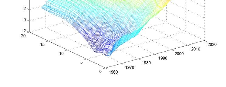
"conventional" view. Figure 4 provides an alternative perspective to the same evidence, by
displaying the evolution over time of the impact of the monetary policy shock on the log
deviations between observed and fundamental stock prices at di¤erent horizons. Figure 5
shows the estimated (bootstrap-based) probability that the same gap is positive. Note that
the probability is well above 50 percent (and often much closer to unity) since the mid-80s.
Figures 6.a-6.d illustrate the changing patterns of stock price responses by showing
the average impulse responses of both observed and fundamental prices over four alterna-
tive three-year periods: 1967Q2-1970Q1, 1976Q1-1978Q4, 1984Q4-1987Q3, and 1997Q1-
1999Q4. The changing pattern of the gap between the two variables emerges clearly. The
response during the …rst episode, from the 1960s, points to a drop of the observed price
larger than that of the fundamental. The evidence from the 1970s suggests a relatively
similar pattern in both responses, though the observed price displays some overshooting
relative to the fundamental. On the other hand, the estimated responses for the three-year
periods before the crash of October 1987, as well as the period before the burst of the
dotcom bubble, point to a very di¤erent pattern: the observed price declines less than the
fundamental to begin with, and then recovers faster to end up in strongly positive territory,
as the theory of rational asset price bubbles would predict when a large bubble is present.
We have re-estimated the model using an alternative sample period ending in 2007Q3,
i.e. leaving out the period associated with the deeper …nancial crisis, a binding zero lower
bound and the adoption of unconventional monetary policies. We have also examined the
robustness of our results to the use of earnings instead of dividends. Even though the latter
is, in principle, the appropriate variable, earnings are often used in applications due to their
less erratic seasonal patterns. In both cases, our …ndings are largely unchanged. Figures
7 and 8 illustrates that robustness by showing the dynamic response of the gap between
the stock price and the fundamental to an exogenous tightening of monetary policy using,
respectively, the shorter sample period and the earnings-based VAR. Note that the observed
pattern of responses is very similar to that found in Figure 3.h, at least qualitatively.
124 Alternative interpretations
4.1 Time-varying equity premium
The theoretical analysis of section 1 has been conducted under the maintained assumption
of risk neutrality or –equivalently, for our purposes– of a constant expected excess return
(or equity premium). That assumption also underlies our de…nition of the fundamental
component of stock prices and of the estimates of the latter’s dynamic response to monetary
policy shocks shown in the previous section. There is plenty of evidence in the literature,
however, of time-varying expected excess return in stock prices, partly linked to monetary
policy shocks.12 Next we examine whether our estimated deviation between observed stock
prices and the "measured" fundamental component can be plausibly interpreted as resulting
from a time-varying equity premium, as an alternative to the bubble-based interpretation.
Let zt+1 denote the (log-linearized) excess return on stocks held between t and t + 1,
given by
zt+1 = qt+1 + (1 )dt+1 qt rt
In the absence of a bubble, we can write the equilibrium stock price
1
X
k
qt = const + [(1 )Et fdt+k+1 g Et frt+k g Et fzt+k+1 g]
k=0
Thus, the dynamic response of the stock price to an exogenous monetary policy shock
is given by
X 1
@qt+k j @dt+k+j+1 @rt+k+j @zt+k+j+1
= (1 )
@"m
t @"m
t @"mt @"m
t
j=0
Then it follows that the gap between the response of the observed price and the response
of the fundamental component computed under the assumption of risk neutrality are related
to the equity premium response according to the equation:
F 1
X
@qt+k @qt+k j @zt+k+j+1
=
@"m
t @"m
t @"m
t
j=0
@q F P1 j @d @rt+k+j
for k = 0; 1; 2; :::and where, as above, @"t+k
m j=0 (1 ) t+k+j+1
@"m @"m is the
t t t
fundamental stock price under risk neutrality.
Thus, an interpretation of the evidence above that abstracts from the possibility of
bubbles and relies instead on a time-varying equity premium requires that the latter declines
substantially and persistently in response to a tightening of monetary conditions. That
12
See, e.g. Thorbecke (1997), Patelis (1997).and Bekaert, Hoerova and Lo Duca (2013).
13implication is at odds with the existing evidence on the response of excess stock returns
(e.g. Patelis (1997), Bernanke and Kuttner (2005)) or variables that should be closely
related to it, like the VIX (Bekaert et al. (2013)).
4.2 Long term rate response
The evidence of a positive response of stock prices to a tightening of monetary policy could
also be reconciled with a fundamentals-based explanation if the observed rise in the federal
funds rate coexisted with a simultaneous decline in the long term interest rate, possibly due
to a (mistaken) anticipation of su¢ ciently lower short term rates further down the road.13
In order to assess that hypothesis we have re-estimated our VAR with the yield on the
10-year government bond replacing stock prices. Figure 9 displays the dynamic response of
the long term rate to a tightening of monetary policy (i.e. to an orthogonalized innovation
in the federal funds rate, as above). The Figure makes clear that the long-term rate rises
persistently in response to the higher federal funds rate. The increase is particularly large
in the period starting in the early 1980s, precisely when the gap between the observed stock
price and its fundamental value shows a larger increase. Thus, the hypothesis that the
observed rise in stock prices is due to a decline in long term rates is not supported by the
evidence.
4.3 Simultaneity
The estimates reported above were obtained under the identifying assumption that the
Federal Reserve did not respond contemporaneously (i.e. within the quarter) to stock price
innovations. That assumption is consistent with the "pre-crisis consensus" according to
which central banks should focus exclusively on stabilizing in‡ation and the output gap.14
Here we examine the robustness of our …ndings to relaxing that constraint, by allowing
for some (contemporaneous) simultaneity in the determination of interest rates and stock
prices. More speci…cally, we re-estimate our empirical model under the assumption that
current log change in stock prices enters the interest rate rule with a coe¢ cient 0:02. This
implies that, ceteris paribus, a ten percentage point increase in stock prices within a quarter
triggers a 20 basis points rise in the federal funds rate. The previous assumption is consistent
with the estimated reaction of monetary policy to the stock market changes obtained by
Rigobon and Sack (2003) using an approach that exploits heteroskedasticity in stock price
shocks to identify the coe¢ cient measuring that reaction.15
13
This possibility was suggested by our discussant Lucrezia Reichlin.
14
It is also consistent with formal evidence in Fuhrer and Tootell (2008) based on estimated interest rate
rules using real time Greenbook forecasts, though that evidence does not rule out the possibility of an indirect
response to stock prices, based on their potential ability to predict output or in‡ation developments.
15
D’Amico and Farka (2011) use an alternative two-step procedure to identify the policy response to
14The estimated responses of interest rates and dividends to a monetary policy shock (not
shown) are not much a¤ected by the use of this alternative identi…cation scheme. But the
same cannot be said for stock prices: with the exception of a brief period in the early 1980s,
the latter now decline persistently throughout the sample period in response to a tightening
of monetary policy, as shown in Figure 10.a. Furthermore, and most importantly for our
purposes, the gap between the observed price and the estimated fundamental price also
declines strongly in response to the same shock, as shown in Figure 10.b. The latter response
is consistent, at least in a qualitative sense, with the conventional wisdom regarding the
impact of monetary policy on stock price bubbles, and contrasts starkly with the evidence
based on our baseline speci…cation.
If one accepts this alternative identifying assumption as correct, the …ndings obtained
in the previous section should be interpreted as spurious, and driven by biased estimates of
matrices fSt g resulting from the imposition of an incorrect identifying assumption. Figure
11 displays the stock price response after four quarters to the tightening of monetary policy,
for four alternative calibrations of the contemporaneous stock price coe¢ cient in the interest
rate rule: 0:0, 0:01, 0:02, and 0:03. We see that estimates of the e¤ects of monetary policy
on stock prices are rather sensitive to the calibration of that parameter. In a nutshell,
the larger is the calibrated stock price coe¢ cient in the interest rate rule, the smaller (i.e.
more negative) is the estimated e¤ect of an interest rate shock on stock prices. That
negative conditional comovement is required in order to compensate for the strong positive
comovement that arises as a result of non-monetary policy shocks, due to the endogenous
policy response to stock price movements embedded in the rule.
The previous interpretation, however, is subject to an important caveat, which calls it
into question. In a recent paper, Furlanetto (2011) has revisited the evidence of Rigobon and
Sack (2003) using data that extends over a longer sample period (1988-2007) and focusing
on the stability over time in the estimates of the monetary policy response to stock prices.16
He shows that the main …nding in Rigobon and Sack (2003) is largely driven by a single
episode: the Fed’s interest rate cuts in response to the stock market crash in 1987. When the
same empirical model is re-estimated using post-1988 data, the estimated policy response
is much smaller or insigni…cant. The Furlanetto evidence has an important implication for
the present paper, for it suggests that our baseline speci…cation is a good approximation,
possibly with the exception of the period around 1987. Given that our empirical framework
stock prices, obtaining a similar estimate of the response coe¢ cient (about 0:02). Furlanetto (2011) revisits
de Rigobon-Sack evidence and concludes that the positive estimated reaction is largely driven by the Fed
response to the stock market crash of 1987.
16
In addition, he also examines the evidence for six other economies (Australia, Canada, New Zealand,
Norway, Sweden and the United Kingdom). He …nds evidence of a signi…cant endogenous response to stock
prices only in Australia.
15allows the model’s coe¢ cients to vary over time, that "transitory" misspeci…cation should
not distort the estimated responses for other "segments" of the sample. On the other hand,
imposing a "…xed" stock price coe¢ cient in the interest rate rule in the absence of an
endogenous policy response would likely distort the estimated model for the entire sample
period.
Thus, and conditional on Furlanetto’s …ndings, our evidence pointing to an eventual
positive (and growing) response of stock prices (in both levels and deviations from funda-
mentals) to a tightening of monetary policy should be viewed as valid, while the estimates
using the alternative speci…cation are likely to be distorted by the imposition of an identi-
fying assumption that is invalid for much of the sample.
5 Concluding Remarks
Proposals for a "leaning against the wind" monetary policy in response to perceived devi-
ations of asset prices from fundamentals rely on the assumption that increases in interest
rates will succeed in shrinking the size of an emerging asset price bubble. Yet, and de-
spite the growing popularity of such proposals, no evidence seems to be available providing
support for that link.
In the present paper we have provided evidence on the response of stock prices to
monetary policy shocks, and tried to use that evidence to evaluate the empirical merits of
the "conventional" view according to which the size of the bubble component of stock prices
should decline in response to an exogenous increase in interest rates.
Our evidence is based on an estimated vector-autoregression with time-varying coe¢ -
cients, applied to quarterly US data. Under our baseline speci…cation, which assumes no
contemporaneous response of monetary policy to asset prices, the evidence points to pro-
tracted episodes in which stock prices increase persistently in response to an exogenous
tightening of monetary policy. That response is clearly at odds with the "conventional"
view on the e¤ects of monetary policy on bubbles, as well as with the predictions of bub-
bleless models. We also argue that it is unlikely that such evidence be accounted for by an
endogenous response of the equity premium to the monetary policy shocks or by "mistaken
expectations" on the part of market participants that might drive long term interest rates
down.
The previous …ndings are overturned when we impose a contemporaneous interest rate
response to stock prices consistent with the evidence in Rigobon and Sack (2003): under
this alternative speci…cation our evidence points to a decline in stock prices in response to
a tightening of monetary policy, beyond that warranted by the estimated response of the
fundamental price. Recent independent evidence by Furlanetto (2011), however, calls into
question the relevance of this alternative speci…cation.
16Further research seems to be needed to improve our understanding of the e¤ect of interest
rate changes on asset price bubbles. That understanding is a necessary condition before
one starts thinking about how monetary policy should respond to asset prices. We hope
to have contributed to that task by providing some evidence that calls into question the
prevailing dogma among advocates of "leaning against the wind" policies, namely, that a
rise in interest rates will help disin‡ate an emerging bubble.
17References
Bekaert, Geert, Marie Hoerova and Marco Lo Duca (2013): "Risk, Uncertainty and Mone-
tary Policy," ECB WP Series no 1565.
Bernanke, Ben S. and Mark Gertler (1999): "Monetary Policy and Asset Price Volatil-
ity," in New Challenges for Monetary Policy, Federal Reserve Bank of Kansas City, 77-128.
Bernanke, Ben S. and Mark Gertler (2001): "Should Central Banks Respond to Move-
ments in Asset Prices?" American Economic Review 91(2), 253-257.
Bernanke, Ben S. and Kenneth N. Kuttner (2005): "What Explains the Stock Market
Reaction to Federal Reserve Policy?," The Journal of Finance 60(3), 1221-1256.
Borio, C. and P. Lowe (2002): "Asset Prices, Financial and Monetary Stability: Explor-
ing the Nexus," BIS Working Papers no. 14.
Carter, Chris K., and Robert Kohn (1994): "On Gibbs Sampling for State Space Mod-
els," Biometrika, 81:541-553.
Christiano, Lawrence J., Martin Eichenbaum, and Charles L. Evans (2005): “Nominal
Rigidities and the Dynamic E¤ects of a Shock to Monetary Policy," Journal of Political
Economy, vol. 113, no. 1, 1-45.
Cecchetti, S.G., H. Gensberg, J.L. and S. Wadhwani (2000): Asset Prices and Central
Bank Policy, Geneva Reports on the World Economy 2, CEPR.
Cochrane, John (2001): Asset Pricing, Princeton University Press (Princeton, NJ).
D’Amico, Stefania and Mira Farka (2011): "The Fed and the Stock Market: An Iden-
ti…cation based on Intraday Futures Data," Journal of Business and Economics Statistics
29 (1), 126-137.
Del Negro, Marco and Giorgio Primiceri (2013): ”Time-Varying Structural Vector Au-
toregressions and Monetary Policy: A Corrigendum” Federal Reserve Bank of New York
Sta¤ Report No. 619.
Fuhrer, Je¤ and Geo¤ Tootell (2008): "Eyes on the Prize: How did the Fed Respond to
the Stock Market?," Journal of Monetary Economics 55, 796-805.
Furlanetto, Francesco (2011): "Does Monetary Policy React to Asset Prices? Some
International Evidence," International Journal of Central Banking 7(3), 91-111.
Gali, Jordi (2014) ”Monetary Policy and Rational Asset Price Bubbles,”American Eco-
nomic Review, forthcoming.
Gali Jordi and Luca Gambetti (2009). "On the Sources of the Great Moderation",
American Economic Journal: Macroeconomics 1(1):26-57
Gelman Andrew, John B. Carlin, Hal S. Stern, and Donald B. Rubin (1995), Bayesian
Data Analysis, Chapman and Hall, London.
Gürkaynak, Refet S., Brian Sack, and Eric T. Swanson (2005): "Do Actions Speak
Louder then Words? The Response of Asset Prices to Monetary Policy Actions and State-
18ments," International Journal of Central Banking 1 (1), 55-93.
Kim Sangjoon, Neil Shepard and Siddhartha Chib (1998),“Stochastic Volatility: Like-
lihood Inference and Comparison with ARCH Models”, Review of Economic Studies, 65,
361-393.
Kohn, Donald L. 2006. "Monetary Policy and Asset Prices," speech at an ECB collo-
quium on "Monetary Policy: A Journey from Theory to Practice," held in honor of Otmar
Issing.
Patelis, Alex D. (1997): "Stock Return Predictability and the Role of Monetary Policy,"
Journal of Finance 52(5), 1951-1972.
Primiceri, Giorgio (2005): "Time Varying Structural VAR and Monetary Policy," Review
of Economic Studies, 72, 453-472.
Rigobon, Roberto and Brian Sack (2003): "Measuring the Reaction of Monetary Policy
to the Stock Market," Quarterly Journal of Economics 118 (2), 639-669.
Rigobon, Roberto and Brian Sack (2004): "The impact of monetary policy on asset
prices," Journal of Monetary Economics 51 (8), 1553-1575.
Samuelson, Paul A. 1958. "An exact consumption-loan model of interest with or without
the social contrivance of money." Journal of Political Economy 66 (6): 467-482.
Santos, Manuel S. and Michael Woodford. 1997. "Rational Asset Pricing Bubbles."
Econometrica 65 (1): 19-57.
Tirole, Jean. 1985. "Asset Bubbles and Overlapping Generations." Econometrica 53
(6): 1499-1528.
Thorbecke, Willem (1997): "On Stock Market Returns and Monetary Policy," The
Journal of Finance 52(2), 635-654.
19Appendix [for online publication only]
The model is estimated using Bayesian MCMC methods. More speci…cally we use the Gibbs
sampling algorithm along the lines described in Primiceri (2005). The algorithm draws sets
of coe¢ cients from known conditional posterior distributions. Under some regularity con-
ditions, the draws converge to a draw from the joint posterior after a burn-in period. Each
iteration of the algorithm is composed of seven steps where a draw for a set of parameters is
made conditional on the value of the remaining parameters. Let wt be a generic (q 1) vec-
tor. We denote wT the sequence [w10 ; :::; wT0 ]0 . Below we report the conditional distributions
used:17
1. p( T jxT ; T ; T ; ; ; ; sT )
2. p( T jxT ; T ; T ; ; ; )
3. p( T jxT ; T ; T ; ; ; )
4. p( jxT ; T ; T ; T ; ; )
5. p( jxT ; T ; T ; T ; ; )
6. p( i jxT ; T ; T ; T ; ; ), i = 1; 2; 3; 4
7. p(sT jxT ; T ; T ; T ; ; ; ) 18
Priors Speci…cation
We make the following assumptions about the priors densities. First, the hyperparameters
, and and the initial states are independent. Second, the priors for the initial states
0 , 0 and log 0 are assumed to be normally distributed. Third, the priors for the hyperpa-
1, 1 and 1
rameters, i are assumed to be distributed as independent Wishart. More
precisely
P ( 0 ) = N (^; 4V^ )
P (log 0) = N (log ^ 0 ; In )
P( i0 ) = N ( ^ i ; V^ i )
1 1 1
P( ) = W( ; )
1 1 2
P( ) = W( ; )
1 1 3
P( i ) = W( i ; i
)
17
Notice that the following ordering of the seven steps is not subject to the problem discussed in Del Negro
and Primiceri (2012).
18
See below the de…nition of sT .
20where W (S; d) denotes a Wishart distribution with scale matrix S and degrees of freedom
d and In is an identity matrix of dimension n n where n is the number of variables in the
VAR.
Prior means and variances of the Normal distributions are calibrated using a time in-
variant VAR for xt estimated using the …rst = 48 observations. ^ and V^ are set equal to
the OLS estimates. Let u ^i+1;t be the residual of the i + 1-th equation of the initial time-
invariant VAR. We apply the same decomposition discussed in the text to the VAR residuals
covariance matrix, ^ = F^ D ^ F^ 0 . log ^ 0 is set equal to the log of the diagonal elements of
D^ 1=2 . ^ i is set equal to the OLS estimates of the coe¢ cients of the regression of u ^i+1;t on
u^1;t ; :::; u ^
^i;t and V i equal to the estimated variances.
We parametrize the scale matrices as follows = 1 ( 1 V^ f ), = 2 ( 2 In ) and i =
3( V ^f
3 i ). The degrees of freedom for the priors on the covariance matrices
1 and 2 are
i
1
set equal to the number of rows and In plus one respectively while 3i is i + 1 for
i = 1; :::; n 1. We assume 1 = 0:005, 2 = 0:01 and 3 = 0:01. Finally V^ f and V^ f are
i
obtained as V^ and V^ i but using the whole sample.
Gibbs sampling algorithm
Let T be the total number of observations, in our case equal to 204. To draw realizations
from the posterior distribution we use T = T =2 observations starting from =2 + 1.19
The algorithm works as follows:
Step 1 : sample T . To draw T we use the algorithm of Kim, Shephard and Chib (1998,
1=2
KSC hereafter). Consider the system of equations xt Ft 1 (xt Wt0 t ) = Dt ut , where
ut N (0; I), Wt = (In wt ), and wt = [1n ; xt 1 :::xt p ]0 . Conditional on xT ; T , and T ,
xt is observable. Squaring and taking logs, we obtain
xt = 2rt + t (17)
rt = rt 1 + t (18)
where xi;t = log(xi;t 2 )20 , i;t = log(u2i;t ) and rt = log i;t . Since, the innovation in (17) is
distributed as log 2 (1), we follow KSC and we use a mixture of 7 normal densities with
component probabilities qj , means mj 1:2704, and variances vj2 (j=1,...,7) to transform
the system in a Gaussian one, where fqj ; mj ; vj2 g are chosen to match the moments of the
log 2 (1) distribution (see Table A1 for the values used).
19
We start the sample from =2 + 1 instead of in order to not to lose too many data points.
20
We do not use any o¤setting constant sine given that the variables are in logs times 100 we do not have
numerical problems.
21Table A1
j qj mj vj2
1.0000 0.0073 -10.1300 5.7960
2.0000 0.1056 -3.9728 2.6137
3.0000 0.0000 -8.5669 5.1795
4.0000 0.0440 2.7779 0.1674
5.0000 0.3400 0.6194 0.6401
6.0000 0.2457 1.7952 0.3402
7.0000 0.2575 -1.0882 1.2626
Let st be a vector whose elements indicate the density to be used for the corresponding
element of t . Conditional on sT , ( i;t jsi;t = j) N (mj 1:2704; vj2 ). Therefore we can use
the algorithm of Carter and Kohn (1994, CK henceforth) to draw rt from N (rtjt+1 ; Rtjt+1 ),
where rtjt+1 = E(rt jrt+1 ; xt ; T ; T ; ; ; ; sT ; ) and Rtjt+1 = V ar(rt jrt+1 ; xt ; T ; T ; ; ; ; sT )
are the conditional mean and variance obtained from the backward recursion equations.
1=2
Step 2 : sample T . Consider again Ft 1 (xt Wt0 t ) = Ft 1 x
^t = Dt ut . Conditional on
T
,x
^t is observable. Each equation of the above system can be written as
x
^1;t = 1;t u1;t (19)
x
^i;t = x
^[1;i 1];t i;t + i;t ui;t i = 2; :::; n (20)
where i;t and ui;t are the ith elements of t and ut respectively and x ^[1;i 1];t = [^
x1;t ; :::; x
^i 1;t ].
Under the assumption that i;t and j;t are independent for i 6= j, the algorithm of
CK can be applied equation by equation to draw i;t from a N ( i;tjt+1 ; i;tjt+1 ), where
t T ; T ; ; ; ) and t T ; T ; ; ; ).
i;tjt+1 = E( i;t j i;t+1 ; x ; i;tjt+1 = V ar( i;t j i;t+1 ; x ;
T
Step 3: sample . Conditional on all other parameters and the observables we have
xt = Wt0 t + "t (21)
t = t 1 + !t (22)
t T; T
tis drawn from a N ( tjt+1 ; Ptjt+1 ), where tjt+1 = E( t j t+1 ; x ; ; ; ; ) and Ptjt+1 =
V ar( t j t+1 ; xt ; T ; T ; ; ; ) are obtained using CK.
Step 4: sample . To draw a realization for we exploit the fact that the conditional
1 is a Wishart distribution with scale matrix 1
posterior of and degrees of freedom 1 .
So = M M 0 where M is an (n2 p + n) 1 matrix whose columns are independent draws
1 PT 0
from a N (0; ) where = + t=1 t( t ) (see Gelman et. al., 1995).
22Step 5 : sample . As above, = M M 0 where M is an n 2 matrix whose columns
1 P
are independent draws from a N (0; ) where = + Tt=1 log t ( log t )0 .
Step 6: sample i . As above, i = M M 0 where M is an i 3 matrix whose columns
1 P
are independent draws from a N (0; i ) where i = i + Tt=1 i;t (
0
i;t ) .
Step 7: sample sT . Each si;t is independently sampled from the discrete density de…ned
by P r(si;t = jjxi;t ; ri;t ) / fN (xi;t j2ri;t +mj 1:2704; vj2 ), where fN (xj ; 2 ) denotes a normal
density with mean and variance 2 .
We make 22000 draws discarding the …rst 20000 and collecting one out of two of the
remaining 2000 draws. The results presented in the paper are therefore based on 1000 draws
from the posterior distribution. Parameters convergence is assessed using trace plots.
23Figure 1
Asset Price Response to an Exogenous Interest Rate Increase:
Alternative Calibrations
6
4
2
asset price response
0
-2
-4
gamma = 0
gamma = 0.5, psi =0
gamma = 0.5, psi = -8
gamma = 0.5, psi = 6
-6
0 5 10 15 20
periods after shockFigure 2
Estimated Responses to Monetary Policy Shocks:
VAR with Constant Coefficients
a. Federal funds rate
b. Real interest rate
c. GDP
d. GDP DeflatorYou can also read