Scholarship @ Claremont - Claremont Colleges - Scholarship ...
←
→
Page content transcription
If your browser does not render page correctly, please read the page content below
Claremont Colleges
Scholarship @ Claremont

CMC Senior Theses                                                                   CMC Student Scholarship

2020

Optimal Execution in Cryptocurrency Markets
Ethan Kurz

Follow this and additional works at: https://scholarship.claremont.edu/cmc_theses

   Part of the Finance Commons, and the Mathematics Commons

Recommended Citation
Kurz, Ethan, "Optimal Execution in Cryptocurrency Markets" (2020). CMC Senior Theses. 2387.
https://scholarship.claremont.edu/cmc_theses/2387

This Open Access Senior Thesis is brought to you by Scholarship@Claremont. It has been accepted for inclusion in
this collection by an authorized administrator. For more information, please contact
scholarship@cuc.claremont.edu.
Claremont McKenna College

 Optimal Execution in

Cryptocurrency Markets

            submitted to

      Professor Benjamin Gillen

                and

       Professor Chiu-Yen Kao

             written by

            Ethan Kurz

            Senior Thesis

            Spring 2020

            May 11, 2020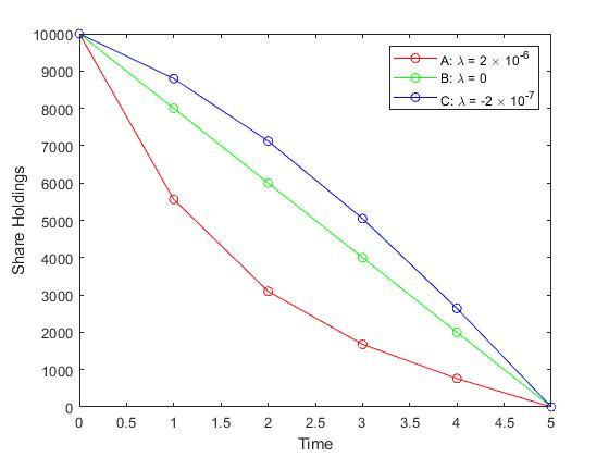
Acknowledgements

I would like to thank my family and friends for keeping my spirits up and being a great support

system. I would also like to extend my deepest gratitude towards my thesis readers, Professor

Benjamin Gillen and Professor Chiu-Yen Kao for their patience and thoughtful guidance throughout

this process.
Contents

1 Abstract                                                                                              1

2 Introduction                                                                                          2

3 Literature Review                                                                                     6

  3.1   Stock Market Microstructure . . . . . . . . . . . . . . . . . . . . . . . . . . . . . . .       6

  3.2   Cryptocurrency Market Microstructure . . . . . . . . . . . . . . . . . . . . . . . . . .        8

  3.3   Microstructure in Almgren-Chriss . . . . . . . . . . . . . . . . . . . . . . . . . . . . .     11

4 Almgren-Chriss model                                                                                 14

  4.1   The “Efficient Frontier” . . . . . . . . . . . . . . . . . . . . . . . . . . . . . . . . . .   14

  4.2   Optimal Strategies . . . . . . . . . . . . . . . . . . . . . . . . . . . . . . . . . . . . .   14

  4.3   Comparative Statics . . . . . . . . . . . . . . . . . . . . . . . . . . . . . . . . . . . .    15

  4.4   NYSE Stock Parameters and Models . . . . . . . . . . . . . . . . . . . . . . . . . . .         18

5 Empirical Analysis of Cryptocurrency Markets                                                         23

  5.1   Choosing Parameters and Modeling . . . . . . . . . . . . . . . . . . . . . . . . . . . .       23

  5.2   Comparison of the Markets . . . . . . . . . . . . . . . . . . . . . . . . . . . . . . . .      25

        5.2.1   Consumer Value Provided by Coinbase . . . . . . . . . . . . . . . . . . . . . .        27

6 Limitations and Further Research                                                                     29

7 Conclusion                                                                                           30

8 Appendix: Matlab Code for Figure 1                                                                   31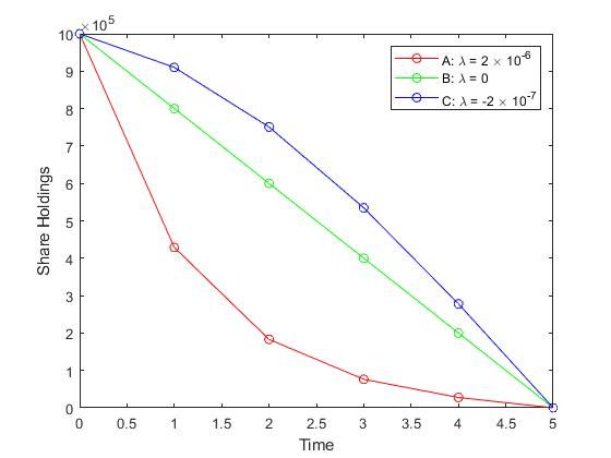
1    Abstract

The purpose of this paper is to study the Almgren and Chriss model on the optimal execution of

large block orders both on the NYSE and in cryptocurrency exchanges. Their model minimizes

execution costs, which include linear temporary and permanent price impacts. We focus on how the

stock market microstructure differs from a cryptocurrency exchange microstructure and what that

means for how the model functions. Once the model and microstructures are explained, we examine

how the Almgren-Chriss model functions with stocks from the NYSE, looking at specifically selling a

large number of shares. We then investigate how a large “wholesale” exchange like Binance has very

different execution costs when compared to a “retail” exchange like Coinbase’s consumer exchange,

and what this means for a trader trying to make a large block order optimally. We examine how

traders should place large orders on Bitcoin exchanges, and quantify the importance of choosing the

right exchange.

                                                1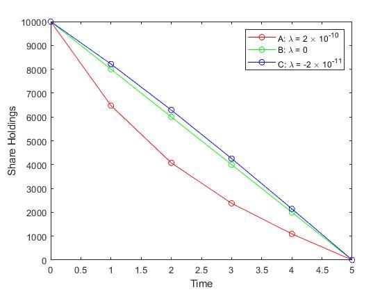
2    Introduction

Optimal portfolio execution refers to the problem institutional traders face when placing large block

orders. Large block orders in layman terms is just the operation of placing a buy or sell order on

a large number of securities. In this paper, our large block orders will be trades of 10,000 or more

shares of a security. These large block orders are known to have both a temporary and permanent

impact on the price as they change the instantaneous supply and demand for that specific security.

This price impact created by large block orders has been studied by Kraus and Stoll in 1972 [13],

Holthausen, Leftwich, and Mayers in 1987 and 1990 [11, 12], and Bertsimas and Lo in 1998 [7].

The optimality condition comes into play when trying to figure out how to find the best trading

trajectory to minimize expected costs, where a trading trajectory is the number of shares sold at

certain times within a set time period.

         Bertsimas and Lo [7] created a model with linear price impacts that focused just on minimiz-

ing the expected costs. Almgren and Chriss [6] built on that model by adding a variance component

and creating a visual representation of the “efficient frontier.” Almgren and Chriss have a subnote

in their paper stating that units of a security can mean, “shares of stocks, futures contracts, and

units of foreign currency.” The novelty of our application of the Almgren-Chriss model is classifying

the security type as cryptocurrencies. According to Fan et al. [10], “Cryptocurrency is a decen-

tralised medium of exchange which uses cryptographic functions to conduct financial transactions,”

and define cryptocurrency trading as, “the act of buying and selling of cryptocurrencies with the

intention of making a profit.” For the purpose of our paper we will be focusing on Bitcoin, the most

traded cryptocurrency, which also has a dominant impact on the cryptocurrency market overall, and

specifically the BTC/USD pair. This would be most similar to investing in a normal NYSE stock

with USD. As of right now, there is no published model on large block order transactions and their

impact in the cryptocurrency market.

         The literature review section will further explain market microstructures, a general back-

ground followed by an explanation of cryptocurrencies and how their market microstructure differs

from a typical stock market. The literature review section will conclude with how the Almgren-

Chriss model incorporates the microstructure with temporary and permanent impact functions.

The Almgren-Chriss Model section will explain the optimization problem and explain how the var-

ious parameters function within the model through examining AMZN and BAC from the NYSE.

The Empirical Analysis of Cryptocurrency Markets section will first explain how we chose the new

                                                 2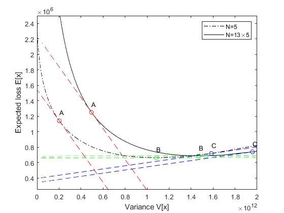
parameters, examine how two cryptocurrency exchanges, Binance and Coinbase, can differ in their

market microstructure, and elaborate on what those differences mean for investors seeking to liq-

uidate their Bitcoin holdings on these exchanges. The following section, Limitations and Further

Research, will examine the limitations of estimating cost of liquidation using this Almgren-Chriss

model in a cryptocurrency market structure and examine possible future research.

         Binance was launched in 2017, and as of writing this paper, Binance is ranked in the

top 20 exchanges by trade volume with over 500 cryptocurrency pairs available to trade on their

platform [2]. Binance has a whole “infrastructure” of apps, including the trading platform, learning

center, charity center, research platform, etc. Binance further advertises on their website to operate

“the world’s leading cryptocurrency exchange.” We chose to analyze Binance as the “wholesale” level

exchange because of their dominance in the market, large volume in the BTC/USD pair, professional

suite of applications and infrastructure, and fee structure.

         Coinbase is the most advertised and “house-hold” exchange in the United States, holding

16.04% of the BTC/USD trading volume over the past 5 years [3]. Coinbase is interesting because

of their offering of several exchange products to choose from, Coinbase “Consumer”, Coinbase Pro,

and Coinbase Prime. They advertise Coinbase as the beginner friendly exchange, Coinbase Pro

as a market similar to Binance where the trader can be a market maker or taker, and Coinbase

Prime as their exchange for institutional investors. We will be focusing on the “lowest” level of

their exchanges, Coinbase “Consumer” itself, which is their mobile app and Coinbase.com. The

Coinbase exchange only has 21 available cryptocurrencies to trade, and only against USD, and the

foreign currencies in EU, UK, and AU/CA/SG [5]. This will be our “retail” exchange that we will

use to compare to an institutional “wholesale” level platform. At the time of writing, Coinbase is

not regulated by the SEC, though “talks” have been happening since 2018. The fee structures for

Binance and Coinbase are listed in Tables 1 and 2. We will examine the expected execution costs of

both Coinbase and Binance further in the Empirical Analysis of Cryptocurrency Markets section.

         The Almgren-Chriss model provides a good foundation for optimal portfolio execution

analysis. Their article has been cited over a thousand times, representing the strong foundation that

their model provides for this type of research. We will use the Almgren-Chriss model as a window

into the behavior of cryptocurrency markets, focusing on what kinds of execution costs are associated

with trading on these markets. With the conclusion of this paper, we can see what direction to go

with regards to optimal execution in a cryptocurrency market microstructure.

                                                  3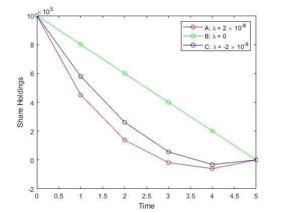
Amount Traded in Last 30 Days   Maker Fees    Taker Fees

                               $200           1.49%

Table 2: contains fee information from help.coinbase.com/en/coinbase/trading-and-funding/pricing-

and-fees/fees.html

                                                 4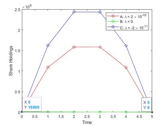
The question of investing in specific cryptocurrency markets becomes significant as in-

stitutional investors begin looking at cryptocurrencies as a viable investment. This paper is an

exploration of how different microstructures will affect how the model works. When comparing two

stocks, AMZN and BAC, we see a large impact from adding a drift term to the model. Looking at

the optimal trajectories, it becomes clear how a negative drift term may actually lead to the trader

shorting shares before the end of the liquidation period. When looking at Binance and Coinbase,

we will see how bid-ask spread plays a large role in execution costs. We find that just the bid-ask

spread provides a great clue as to how an institutional investor may select an exchange. We also

calculate a numerical value for the “consumer value” provided by Coinbase.

                                                 5
3 Literature Review
3.1 Stock Market Microstructure
What is a stock market microstructure? The market microstructure focuses on how assets are
transferred between investors and what costs are incurred in this process. In a stock exchange like
the NYSE, the focus of our analysis on stock markets, there are a few main elements: investors,
brokers, dealers, and the market itself. According to Stoll, in Chapter 9, “Market Microstructure”, of
The Handbook of the Economics of Finance, “investors are the ultimate demanders and suppliers of
immediacy and the brokers and dealers facilitate trading” [8]. Brokers make a commission, whereas
dealers trade for their own accounts. The dealer in the NYSE is the “specialist” who, “maintains
liquidity by trading with brokers representing public customers” [8]. The market itself is a place
where buyers and sellers can congregate with a majority of this happening electronically now.
The NYSE operates as a continuous auction market, with a “crowd” consisting of, “in-
vestors, who wish to sell, trade at the bid price established by resting buy orders or at prices in
the ‘crowd’, and investors, who wish to buy, trade at the asking price established by resting sell
orders or at prices in the ‘crowd’” [8]. The “crowd” are the floor brokers. What makes the NYSE a
mixed auction and dealer market is the specialist trading their own accounts, instead of a completely
continuous auction market like most electronic exchanges including Forex and Bitcoin.
The NYSE functions as a centralized exchange where specialists are assigned a stock and
are the market makers for that stock. The specialists receive the trades electronically and on the
floor, but much less arrives physically from the floor anymore. The most common orders they receive
come as a market order or a limit order. The market order trades at the best price available whereas
the limit order sells at a specified limit or better. In the NYSE, the limit order book, LOB, is
determined by the best limit order to buy and sell the stock. The number of shares being traded at
those prices is the depth of the market.
Large orders can be traded as blocks, which, “are often pre-negotiated “upstairs” by a
broker who has identified both sides of the trade. The trade is brought to a trading floor, as
required by exchange rules and executed at the pre-arranged prices” [8]. According to Investopedia,
a block trade is typically 10,000 shares or assets totalling $200,000. Institutional investors are the
ones usually making these larger orders, whereas the individual investor, who makes the majority
of intraday trades, makes smaller trades. As a result of their large orders, institutions have to deal
6with interesting minimization of execution cost problems. On the NYSE, large block orders, “must
be brought to the floor, where resting limit orders and floor brokers. . . must be satisfied, further
the block trade must be reported publicly” [8]. When selling a large block order, Kraus and Stoll
have found evidence of temporary price impact. There is also a permanent price impact, where the
price does not “bounce back” after a block order, which means that block orders are also a source
of signalling new information.
The NYSE has a couple rules for precedence, which outline how and who execute against
the incoming market orders. They have parity, “a unique tool for allocation of liquidity”, where ,
“at each price level, the Electronic Book, the DMM and each floor broker are eligible to participate
in an execution on a parity basis” [4]. This allows institutional investors to share executions at the
same time as high frequency traders. The NYSE also has “setting priority” rules where, “the setter
of the best quote receives 15% of each trade at that price until the setter’s order is filled, plus its
parity share” [4].
The trading process on the NYSE has 4 distinct parts, information, routing, execution,
and clearing. Information is shared about the stock prices in real time to the public. Trades are
routed by the specialists, which arrive to the specialist at the NYSE through a DOT, designated
turnaround system. They are then executed by the specialists who, “are reluctant to execute orders
automatically. . . instead, they prefer to delay execution, if even for only 15 seconds, to determine if
any information or additional trades arrive,” making this a complex step [8]. Execution is followed
by clearing where comparisons of transactions between buying and selling orders are made.
Microstructure theory focuses mainly on the bid-ask spread, and impacts to the LOB,
which is where we will also be focusing. The bid-ask spread, “is an indicator of the cost of trading
and the illiquidity of a market” [8]. There are a few factors that help create the bid-ask spread. The
specialists, who create the supply of liquidity, have operating costs, as they are physical employees.
This would be different on a cryptocurrency market where there are no specialists that incur handling
costs. The spread can also have minimum tick sizes to increase spreads. The main focus of past
literature is, “the effect of asymmetric information. If some investors are better informed than
others, the person who places a firm quote (bid or ask) loses to investors with superior information”
[8].
Order flow imbalance, where there is a greater demand or supply of the asset, more bids
than there are asks or visa versa, also has price impact implications. This imbalance ties the bid-ask
7spread in with large market orders in the sense that large block orders have an impact on price
because the trade increases the supply quickly of a stock, lowering the price.
There are three main factors that deal with uncertainty in the market: inventory risk,
option effect, and asymmetric information. Inventory risk has to do with the risk the trader faces
of the assets changing value negatively after they have been bought or sold. The option effect is the
opposite, information about the asset changes negatively, but the price cannot be changed before
trade execution. The asymmetric information effect was mentioned above, where a trader is trading
with more knowledge than the other traders.
Within a market, there are other factors separate from the actual bid-ask spread to consider,
such as anonymity, transparency, automation, and tick sizes. According to Stoll, “in an anonymous
market, dealers and limit orders must lose to informed traders, for the informed traders are not
identified.” Anonymous traders exist on the NYSE, and these are large traders who want to avoid
making market signals. With regards to transparency, NYSE shows the “top of the book,” the best
bid and ask. “The ESNs display the entire book” [8]. Transparency is important because it increases
market efficiency, where no single investor has an advantage and everyone sees the same information.
On the NYSE, this also helps the individual investors to make sure their broker is making the right
trades for them, and not taking advantage of them. This is also important for brokers and dealers
to be able to increase competition between each other, as they compete to offer lower commission
or spread. Automation has an interesting impact because with automation there is no room for
negotiation. The NYSE has an automatic routing system, but the specialist still holds the option
to change the quote. Tick size, “is the minimum allowable price variation in a security.” This is
important because it directly impacts the spread, with a $0.01 tick size on the NYSE, “many stocks
trade at a spread of 5 cents or less” [8].
3.2 Cryptocurrency Market Microstructure
In 2017, around the time Bitcoin was making a record run in price, big banks were skeptical of the
feasibility of investing in cryptocurrencies. Times have changed, and in late 2019, articles from Coin-
desk, Cointelegraph, and various other cryptocurrency news sources suggest institutional investors
are beginning to trade in cryptocurrencies, making the optimal execution problem relevant. In ad-
dition to concerns of price manipulation, institutional investors must also consider the underlying
price volatility in cryptocurrencies. According to Puljiz et al., “understanding market microstructure
8and investor behavior is a key step towards safer and improved implementations of cryptocurrency
exchanges, especially when considering the risks of extreme price fluctuations” [16]. For the purpose
of this paper, we will examine Bitcoin, the most established and “stable” cryptocurrency.
Cryptocurrency exchanges are platforms that either function as market makers or a “match-
ing platform, by simply charging fees” [10]. Coinbase is one interesting exchange/company, their
other higher level exchanges are matching platforms, but “Coinbase Consumer quotes a price and
then quickly fills the order from our exchange platform (Coinbase Markets)” [14]. Binance, however,
is a straightforward matching platform that charges maker and taker fees. There are many different
exchanges to choose from because of the nature of blockchain and the common API all cryptocurren-
cies share. Each exchange vies to offer something the other exchange does not to attract customers.
Coinbase attempts to get beginners in the cryptocurrency world to use their simple platform and
set up a wallet on there. Their ease of use may make it more attractive to some than Binance, but
for someone who wants lower fees and understands how the market works, Binance may be a better
option. The existence of many cryptocurrency exchanges is beneficial to the individual trader, as
more competition leads to lower execution costs as the exchanges vie for traders.
Binance is a continuous double auction, which means that bid and ask orders are auto-
matically matched on the electronic exchange. There is no dealer intervention, with no specialists
or brokers interfering with individual traders. Coinbase once again is an interesting case: their
Consumer exchange seems to be a dealer market that is tied into their other continuous auction
markets. It is a dealer market because Coinbase makes a fee on the trade and also adds a margin
to the spread [5].
Large orders are just folded into the limit order book as the trader wishes, there is no
external dealer who attempts to negotiate prices or limit market impact for the trader. It is up to
the individual trader who is making the order to figure out the best way to handle it for themselves,
and according to Silantyev there is empirical evidence that “traders (are) splitting their orders into
multiple smaller orders” [17]. On Binance, their fee structure encourages larger volumes being traded
over 30 days with lower maker and taker fees, see Table 1. Coinbase, on the other hand, has a flat
fee of 1.49% after $200.
The trading process on a cryptocurrency exchange is pretty simple. On Coinbase, the
trader clicks the trade button and tells the exchange how much Bitcoin they would like to buy or
sell. There is no option to choose the type of order. Binance, on the other hand, has several trading
9options. They have a P2P option, where the trader can trade directly with a peer, taking out the
financial institution completely, as well as the standard order options of limit, market, or stop-limit
orders. Binance provides clear advantages to the sophisticated trader with having more options, but
Coinbase is much simpler to get started trading.
The main bid-ask spread factors in a cryptocurrency market that we will focus on are
liquidity, temporary impact, and permanent price impact. Remember, the greater the bid-ask
spread, the more illiquid a security is. We will discuss the exact numbers in the Cryptocurrency
Parameters section, but in general because of the high frequency and automatic matching nature
of cryptocurrencies, the bid-ask spreads on most exchanges are pennies, even though the value of
Bitcoin is in the thousands. This means that Bitcoin is very liquid.
The imbalance of limit order book in cryptocurrencies has a price impact. Silantyev in-
terprets his order flow imbalance model, “for 10,000 units of net trade flow, the expected average
mid-price change is 0.14 ticks” [17].
Uncertainty in cryptocurrency markets comes from the standard inventory risk and option
effect, but much more shows up in asymmetric information than in a normal stock market. Pump
and dumps occur on new cryptocurrencies because the creators or organizers have asymmetric in-
formation. The fear of asymmetric information also leads to large price fluctuations in Bitcoin itself.
The large runs and subsequent crashes have all been news driven.
The factors of anonymity, transparency, automation, and tick sizes are also all different
from a standard market like the NYSE. The trading of cryptocurrencies are fully anonymous with
no reports made to the SEC or other regulating body. The amount of Bitcoin or any other cryp-
tocurrencies any individual institution or individual has in their wallet is also fully anonymous. The
transparency of the order book is higher than the NYSE, as all traders on an exchange like Binance
can see the full depth. The transparency on Coinbase, however, is less so, as there is no order
book the trader can see. Everything about cryptocurrency exchanges are fully autonomous with no
human broker or dealer in the process. The tick sizes, on both cryptocurrency exchanges and the
NYSE, however are the same at a penny.
The impact of technology in cryptocurrency markets is interesting in and of itself. The
ability for almost any educated investor to trade at high frequencies through algorithms simply
hooked up to API, which Binance has readily available API with documentation, leads to more
of such systems being used on many cryptocurrency exchanges. The ability for an individual to
10choose between being a market maker or taker and the subsequent maker and taker fees is also an
interesting technological development not possible on the NYSE.
3.3 Microstructure in Almgren-Chriss
As mentioned previously, when institutional investors make trades, specifically large block orders,
the price of the security is affected. Identifying this effect was the purpose of Kraus and Stoll’s
paper [13]. They hypothesized that there were three reasons price would change: information, short
run liquidity cost, and “different investor preferences for a given security”. The different investor
preferences relates to the large institutional investors versus the small personal investors. Empirically
they claimed the large investors would change the expected rate of return uniquely, “the expected
rate of return must increase in the case of sales to convince less willing buyers to hold the security
and must fall in the case of purchases to convince less willing sellers to part with the security” [13].
This change in the expected rate of return was different from an information or short run liquidity
effect. They concluded, “the actions of institutions do indeed affect market prices” [13].
There is both a temporary and permanent effect from these institutional investors. Holthausen,
Leftwich, and Mayers define these effects nicely: “the temporary price effect is the price rebound
of a security following a block transaction and the permanent price effect is the change from the
equilibrium price before the block trade to the equilibrium price afterwards” [12]. Our model with
Almgren and Chriss follows that. The Almgren-Chriss model has two linear price functions, for
permanent and temporary price impact. Holthausen et al. conclude that, “the speed of adjustment
is a function of the size of the block” [12]. Their paper also shows that the permanent and temporary
price effect increases with the size of the trade, regardless of whether it is a buy or sell order. As
will soon become apparent, the functions that Almgren and Chriss apply are based on the size of
the trade.
The Almgren-Chriss model [6] focuses on the sell side of trading a single security, but “the
definition and results for a buy program are completely analogous.” We begin with holding X units
of a security, with the goal of liquidating it before time T . T is broken into N intervals with the
length τ = T /N .
Using this notation, discrete times are defined as tk = kτ where k = 0, ..., N . They define
the “trading trajectory”: x0 , ..., xN where xk is the units of the security held at time k with x0 = X
at time 0 and xN = 0 at time T . The “trade list” is defined as n1 , ..., nN where nk = xk−1 − xk
11which is related to the “trading trajectory” by:
k
X N
X
xk = X − nj = nj for k = 0, ..., N .
j=1 j=k+1
They define the trading strategy itself as, “a rule for determining nk in terms of information available
at time tk−1 .
Almgren-Chriss model the price of the security based on a discrete arithmetic random walk.
Their formula is:
nk
Sk = Sk−1 + στ 1/2 ξk − τ g( ) for k = 0, ..., N. (1)
τ
Where Sk is the price of the security at time k, σ is volatility, ξk “draws from independent random
variables each with zero mean and unit variance,” and g(v) is the permanent price impact which
nk
depends on the average rate of trading v = τ . This pricing model has no drift term, but we will
add one when we analyze stocks and Bitcoin with this model in later sections [6].
For the permanent impact, Almgren and Chriss use the equation g(v) = γv where γ is the
“daily volume 5 million shares”, with the units $/share2 . When we plug in n as v we decrease the
price per share independent of time, making it a permanent effect. This aligns with the permanent
effect described by Holthausen et al. [12], the permanent impact is a function of n and as n increases,
the effect is clearly also increased.
For the temporary impact, Almgren and Chriss use the equation with a sign function sgn:
nk η
h( ) = sgn(nk ) + nk .
τ τ
If the institution is selling shares, the sign function is positive; and negative if the shares are being
bought instead.
Multiplying n to both sides of the equation gives us “the total cost incurred by buying
or selling n units in a single unit of time” [6]. is the fixed costs, which can be interpreted as
the bid-ask spread, and is in $/share units. η is the impact at 1% of market and is in units of
($/share)/(share/day). This small impact function is supported by the conclusion of Holthausen et
al., “though a small temporary price effect exists and both increase with the size of the block” [12].
Putting the temporary price impact into our pricing model gives us a new variable S̃k =
Sk−1 − h( nτk ). Almgren and Chriss define the “capture of a trajectory to be the full trading revenue
upon completion of all trades” [6].
N N N
X X nk X nk
nk S˜k = XS0 + (στ 1/2
ξk − τ g( ))xk − nk h( ). (2)
τ τ
k=0 k=1 k=1
12As mentioned before, XS0 is the initial market value of the position, from which we add or subtract
P 1/2 P
the volatility στ ξk xk , the permanent market impact − τ xk g(nk /τ ), and the temporary
nk S˜k “between the initial
P P
market impact nk h(nk/τ ). “The total cost of trading” is XS0 −
book value and the capture”.
E(x) is the expected shortfall and V (x) is the variance of the shortfall.
N N
X nk X nk
E(x) = τ xk g( )+ nk h( ). (3)
τ τ
k=1 k=1
N
X
V (x) = σ 2 τ x2k . (4)
k=1
When they add the linear cost functions h( nτk ) and g(v), the expectation shortfall becomes:
N N
1 X η̃ X 2
E(x) = γX 2 + |nk | + nk . (5)
2 τ
k=1 k=1
where η̃ = η− 12 γτ . E is in dollars, V is dollars squared [6]. The goal is now to minimize E(x)+λV (x)
for different λ, which will be explained in the following section.
134 Almgren-Chriss model
4.1 The “Efficient Frontier”
The efficient frontier is generated by optimizing our expected shortfall against the variance. Almgren
and Chriss, “define a trading strategy to be efficient or optimal if there is no strategy which has
lower variance for the same or lower level of expected transaction costs.” To solve min E(x),
x:V (x)≤V∗
Almgren and Chriss use a Lagrange multiplier λ giving us the optimization problem that we will
focus on:
min(E(x) + λV (x)) (6)
x
where λ can be interpreted as risk-aversion. A positive λ refers to a risk-averse strategy, whereas
a negative λ refers to a risk-seeking strategy. We keep the linear price impact functions because
according to Almgren and Chriss, “we may write the solution explicitly and gain a great deal of
insight into trading strategies” [6].
4.2 Optimal Strategies
We solve for the unique global minimum of E(x) + λV (x) by setting the partial derivative equal to
zero.
∂U xj−1 − 2xj + xj+1
= 2τ {λσ 2 xj − η̃ }. (7)
∂xj τ2
where j = 1, ..., N − 1. When partial derivatives equal zero, we can rearrange terms to give
1
(xj−1 − 2xj + xj+1 ) = κ̃2 xj . (8)
τ2
λσ 2 λσ 2
where κ̃2 = η̃ = η(1− γτ
. Using the boundary conditions of x0 = X and xN = 0 gives the trading
2η )
trajectory:
sinh(κ(T − tj ))
xj = X with j = 0, ..., N . (9)
sinh(κT )
with the corresponding trade list:
2 sinh( 12 κτ )
nj = cosh(κ(T − tj− 21 ))X with j = 1, ..., N . (10)
sinh(κT )
E(X) and V (X) then become:
1 tanh( 12 κτ )(τ sinh(2κT ) + 2T sinh(κτ ))
E(X) = γX 2 + X + η̃X 2 . (11)
2 2τ 2 sinh2 (κT )
1 2 2 τ sinh(κT ) cosh(κ(T − τ )) − T sinh(κτ )
V (x) = σ X . (12)
2 sinh2 (κT ) sinh(κτ )
14As κ → 0, ∞, respectively, the equations reduce to the “minimum impact”, where units are sold at
a constant rate over the whole liquidation period, and “minimum variance”, where all units are sold
in the first period. For the minimum impact case, we have
1 1 X2
E= γX 2 + X + (η − γτ ) , (13)
2 2 T
and
1 2 2 1 1
V = σ X T (1 − )(1 − ). (14)
3 N 2N
For the minimum variance case, with conditions n1 = X, n2 = . . . = nN = 0, x1 = . . . = xN = 0:
X X2
E = Xh( ) = X + η . (15)
T τ
and
V = 0. (16)
Using the minimum impact and minimum variance as our boundary conditions, we can
analytically optimize E(x) + λV (x) giving us our optimal trajectories when we plot xj in formula
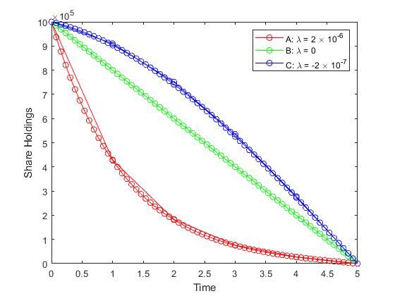
(9) versus tj for various λ seen in Figure 1 (b). The positive λ = 2 × 10⁻⁶ , “represents a risk-averse
trader who wishes to sell quickly to reduce exposure to volatility risk, despite the trading costs
incurred in doing so” [6]. On the other hand, the trading trajectory for λ = −2 × 10⁻⁷ represent a
risk-seeking trader who waits to sell, which leads to higher variance and more expected costs due to
the quick sales at the end. The trading trajectory of λ = 0 is a “simple linear reduction of holdings
over the trading period. This is never an optimal strategy, because one can obtain substantial
reductions in variance for a relatively small increase in transaction costs” [6].
In Figure 1(a), the efficient frontier is constructed from the parameters in Table 3 from
the Almgren and Chriss’ paper, not including the α drift term. In Figure 1(b) the optimal trading
strategies at the λ points selected from the Efficient Frontier. We will treat Figure 1 as our baseline
and do comparisons from here. Note that there is no drift term α when we create these figures. This
drift term will be discussed in the following subsection.
4.3 Comparative Statics
From these baselines shown in Figure 1, we examine the changes we make to parameters independent
of stock specific parameters: trading times, liquidation time, and initial holdings in the following
subsection.
15Variable Name Variable Value
Initial stock price: S0 50 $/share
Initial holdings: X 106 shares
Liquidation time: T 5 days
Number of time periods:: N 5
1/2
30% annual volatility: σ 0.95 ($/share)/day
Bid-Ask spread = 1/8: 0.0625 $/share
2
Daily volume 5 million shares: γ 2.5 × 10⁻⁷ $/share
Impact at 1% of market: η 2.5 × 10⁻⁶ ($/share)/(share/day)
Table 3: holds the exact parameters for the test case from the Almgren and Chriss paper [6].
(a) Efficient Frontier (b) Optimal Trajectories
Figure 1: shows the efficient frontier and the optimal trajectories given by the parameters from
the Almgren and Chriss paper [6]. The Matlab code to generate these figures can be found in the
Appendix.
We first change the trading times from once daily to every half hour. This changes N from
5 to 65. We can see the efficient frontier in Figure 2(a) shifts to the right. This shift represents
higher variance because there is more inventory risk. The increase in options to trade increases
the possibility of the price changing after the shares have been sold already. Because the trader
confronts their higher position more often they have greater liquidation anxiety.
The optimal trajectory in Figure 2(b), when compared to Figure 1(b), simply has more
16(a) Efficient Frontier (b) Optimal Trajectories
Figure 2: illustrates the shift in the curve generated by changing trading times from once daily
(N = 5) to every half hour (N = 13 ∗ 5). This figure, as well as the following figures, can be
replicated by changing the parameters in the Matlab code found in the Appendix.
dots representing more trades. There is no change in slope because the quantities of stocks sold by a
certain point in time remain the same. This is because the model is discrete, we do not see changes
continuously.
(a) Efficient Frontier (b) Optimal Trajectories
Figure 3: examines the difference that an extra week of trading makes.
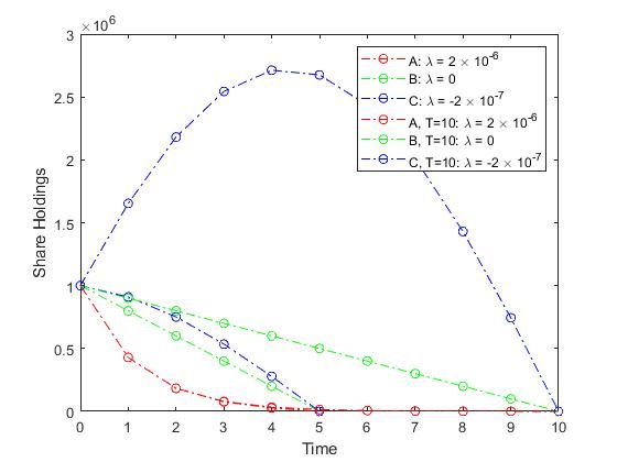
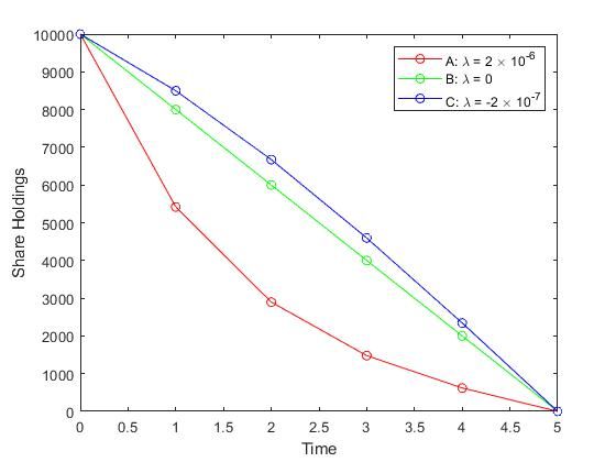
When we change the liquidation time from 1 week to 2, while keeping daily trades (T = 5
and N = 5 to T = 10 and N = 10), we can see a change in both the efficient frontier and optimal
trajectories in Figure 3. Looking at the optimal trajectories in Figure 3(b), in the λ = 0 case
we can see the trader still offloads the shares in a linear form, with a corresponding shift for the
17extended time. The risk-averse trader follows almost the exact same trading trajectory as their
goal is still to offload the shares as quickly as possible while minimizing execution costs. The risk-
seeking trader, however, changes; the risk-seeking investor is not shown in the range of our efficient
frontier graph, but is at approximately V(x) = 3.7 × 10¹³ and E(x) = 6.3 × 10⁶ . This explains the
corresponding extreme trajectory in Figure 3(b). The risk-seeking trader has extreme preferences
given the extended time horizon and thus buys even more shares before offloading shares quickly.
The Efficient Frontier in Figure 3(a) seems to expand due to the loosened constraint on
the duration over which the trading plan must be executed, while keeping the number of shares to
be liquidated the same.
(a) Efficient Frontier (b) Optimal Trajectories
Figure 4: illustrates the shift in the curve generated by changing initial holding (X = 105 vs
X = 106 ),
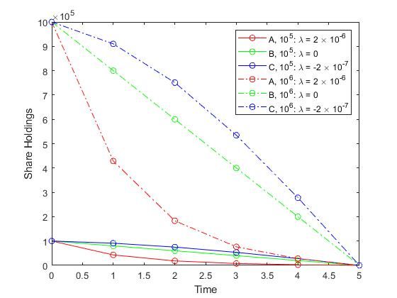
The effect of changing the last non-stock specific parameter of initial holdings from 1, 000, 000
to 100, 000 can be seen in Figure 4. This change only affects the scale but not the shape of the curve
in the Efficient Frontier, Figure 4(a). The curve is just scaled diagonally, but with no change to the
shape itself. The optimal trajectories are also scaled according to the holdings, changing the slope
of the optimal trajectories naturally.
4.4 NYSE Stock Parameters and Models
Before we can examine what happens when we change stock specific parameters, we are going to add
the drift term to the model. This was discussed in Almgren and Chriss’ paper to be, “convenient to
regard a drift parameter in a price process as a directional view of price movements” [6]. We add
18+ατ to the price dynamics equation Sk (1), which changes our E(x) from equation (5) to:
N N N
1 X X η̃ X 2
E(x) = γX 2 − α τ xk + |nk | + nk . (17)
2 τ
k=1 k=1 k=1
The variance does not change, which gives a new optimal solution:
sinh(κ(T − tj )) sinh(κ(T − tj )) + sinh(κtj )
xj = X + 1− x̄ (18)
sinh(κT ) sinh(κT )
where
α
x̄ = .
2λσ 2
We can now evaluate the optimal trading policy and market impact using parameters
calibrated for a specific stock. We examine AMZN (Amazon), a relatively expensive stock, and
BAC (Bank of America), a stock lower than $50 as of December 31, 2019. We will keep the
T = 5 and N = 5 because we explained what changes in those parameters do already, focusing
instead on the stock specific parameters. The data was taken from the WRDS CRSP database,
with the parameters: daily price, volume, return, and the closing bid and ask price. The data
was from January 3, 2007 to December 31, 2019. We calculated the daily volatility by taking the
standard deviation of the daily returns from January 1, 2018 to December 31, 2019. For AMZN
we got 1.90% and for BAC we got 1.51%. We computed the Compound Annual Growth Rate
end price 1/n
(CAGR) using the formula: CAGR = start price − 1, where n was 13 years (2007 to 2019).
The CAGR for BAC was −3.14% and 34.63% for AMZN, which means the fractional returns were
−0.0314/252 = −1.2460 ∗ 10−04 and 0.3463/252 = 0.0014 respectively. The average daily volume
for BAC was 61, 074, 905 and AMZN was 4, 766, 187. The average price for BAC was $30 and
$1716 for AMZN. Using this information we calculate σ, the daily volatility ∗ price, as being equal
to 32.6040 for AMZN and 0.4530 for BAC. We calculate α, the fractional returns ∗ price, as being
equal to −0.0037 for BAC and 2.4024 for AMZN.
We choose to equal half the bid-ask spread, which we calculated from the averages in
2018-2019 to equal 0.005 for BAC and 0.25 for AMZN. We calculate η with the formula:
(bid-ask spread)/(0.01 ∗ daily volume).
This calibration implies that trading 1% of the daily volume induces a cost equal to the bid-ask
spread. η for AMZN is 1.04906 ∗ 10−5 and 1.63733 ∗ 10−8 for BAC. Remember η and are used in
the temporary price impact formula.
19Variable Name Variable Value
Initial stock price: S0 30 $/share
Initial holdings: X 106 shares
Liquidation time: T 5 days
Number of time periods:: N 5
1/2
1.51% daily volatility: σ 0.4530($/share)/day
Bid-Ask spread = 0.01: 0.005 $/share
2
Daily volume 61 million shares: γ 1.63733 × 10⁻⁹ $/share
Impact at 1% of market: η 1.63733 × 10⁻⁸ ($/share)/(share/day)
-3.14% annual growth: α −0.0037($/share)/day
Table 4: holds parameters for BAC.
For the permanent price impact function, we have the γ parameter which is equal to
(bid-ask spread)/(0.1 ∗ daily volume).
This follows the “common rule of thumb that price effects become significant when we sell 10% of
the daily volume” [6]. This gives us a γ = 1.63733 ∗ 10−9 for BAC and = 1.04906 ∗ 10−6 for AMZN.
The parameters for BAC and AMZN are summarized in Tables 4 and 5, respectively. Using
these parameter, we create Figures 5 and 6 as the stock specific analogs to Figure 1. When looking at
just the parameters in Tables 4 and 5, it is clear that while they are close in daily volatility, AMZN
has a much greater annual growth rate. The difference in annual growth rate is significant, as
BAC’s is much smaller and negative. The difference in bid-ask spread can be attributed to AMZN’s
greater price and so is not the main reason the γ and η are different magnitudes. The difference in
volume where BAC has approximately 12 times more volume than AMZN, explains the difference
in magnitude of the permanent and temporary price impact terms γ and η. The extreme difference
in volume can be explained by the fact that AMZN stock price is almost 60 times the BAC stock
price. Less investors are able to trade AMZN stock at the same volume they would be for BAC.
This illiquidity takes form in the bid-ask spread, and we’ve gone full circle in our examination of the
parameters.
When we look at the efficient frontier in Figure 5(a) for BAC, take note that it is positive.
The optimal trading trajectories in Figure 5(b) show both the risk-averse and risk-seeking traders
20Variable Name Variable Value
Initial stock price: S0 1716 $/share
Initial holdings: X 106 shares
Liquidation time: T 5 days
Number of time periods:: N 5
1/2
1.90% daily volatility: σ 32.6040($/share)/day
Bid-Ask spread = 0.5: 0.25 $/share
2
Daily volume 4.8 million shares: γ 1.04906 × 10⁻⁶ $/share
Impact at 1% of market: η 1.04906 × 10⁻⁵ ($/share)/(share/day)
34.63% annual growth: α 2.4024($/share)/day
Table 5: holds parameters for AMZN.
(a) Efficient Frontier (b) Optimal Trajectories
Figure 5: uses the parameters specific to BAC, to create this efficient frontier and optimal trajecto-
ries.
wishing to offload their shares sooner than later with the dip under 0 share holdings indicating a
short position. This phenomena is an artifact of the negative drift. Investors are trying to place a
short position ahead of the terminal period to take advantage of the negative drift.
What’s especially interesting about the efficient frontier in Figure 6(a) for AMZN is that
it goes negative. The significance of a negative expected cost or loss is the fact that money is being
made through the trading process. This result can be attributed directly to the 34.63% annual
21(a) Efficient Frontier (b) Optimal Trajectories
Figure 6: uses the parameters specific to AMZN, to create this efficient frontier and optimal trajec-
tories.
growth rate. The α term of 2.4 pulled the E(x) in equation (18) negative. Compared with the
positive expected loss in Figure 5(a) for BAC, it is clear why trading in a positive drifting stock is
more favorable for the trader when focusing on execution costs.
The optimal trajectories in Figure 6(b) for AMZN are interesting as the risk-averse trader
follows almost a linear path and the risk-seeking trader buys shares near the start of the liquidation
period. These interesting trajectories can be explained by the high drift term. The risk-seeking
trader wishes to buy more stocks before liquidating their stocks to make extra money and thus
lower execution costs. The risk-averse trader follows close to the linear path because of the lower
temporary and permanent impact costs. AMZN’s optimal trajectories are very different than BAC’s
trajectories, which called for shorting the stock before the end of the liquidation period.
When we compare Figure 5 and 6, we see the impact of a negative drift term versus
a positive drift term. Not only does it show up in the fact that AMZN has a expected gains
from trading, when we compare the optimal trajectories in Figure 5(b) to Figure 6(b) we see how
differently the traders act.
225 Empirical Analysis of Cryptocurrency Markets
5.1 Choosing Parameters and Modeling
For choosing our non-security specific parameters X, T , and N , we choose to have initial holdings
of 104 shares because the Almgren-Chriss model held $50, 000, 000 of shares, which when divided
by $7,000 gives us approximately 104 ; even though cryptocurrencies can be traded 24/7, we keep
our timing to daily trades over 5 days: T = 5 and N = 5. To see if there are any differences in
cryptocurrency exchanges, we will compute parameters for both the consumer Coinbase exchange
and the more “robust” Binance exchange.
We acquired the data for the parameters in cryptocurrency model for Coinbase from
data.bitcoinity.org. When looking at the trading volume over the past 5 years, specifically the
BTC/USD pair, we see that Coinbase has 16.04% of all trades against the exchanges listed on
data.bitcoinity.org. One thing to note is Binance and other large exchanges are not listed on
data.bitcoinity.org. From the menu on data.bitcoinity.org, the data for average price and aver-
age spread data from 1/1/2016 to 12/31/2019. The parameters calculated can be seen in Table
6. CAGR, σ, γ, and the other parameters were calculated just like they were in the the Stock
Parameters section.
Data concerning Binance’s Bitcoin prices came from www.CryptoDataDownload.com. Here
we got historical price data from 1/1/2018 to 12/31/2019 and calculated returns and daily volatility.
Hodl.bot.io reports the average bid ask spread being $0.021 [18]. This number looks familiar when
just taking a cursory glance at the charts provided on Binance.com. Because we were not able to
get historical data for the same time period as Coinbase from Binance, we used the same CAGR,
which is acceptable because both exchanges were trading the BTC/USD pair. The parameters for
Binance are compiled in Table 7. Note we held the initial price the same between both exchanges,
and the major differences were the daily volatility and bid-ask spread parameters.
What is immediately interesting with these parameters is the difference in bid-ask spread.
This is an important part of market microstructure. Coinbase has a drastically larger bid-ask spread
than Binance. This can be attributed to the fact that they take a dealer fee on the margin as they
match their consumer trades with their other markets. According to their help site, “Coinbase
charges a spread of about one-half of one percent (0.50%) for cryptocurrency purchases and cryp-
tocurrency sales. However, the actual spread may be higher or lower due to market fluctuations in
23Variable Name Variable Value
Initial stock price: S0 7500 $/share
Initial holdings: X 104 shares
Liquidation time: T 5 days
Number of time periods:: N 5
1/2
3.33% daily volatility: σ 249.88($/share)/day
Bid-Ask spread = 44.52: 22.26 $/share
2
Daily volume 13,107 shares: γ 0.03397$/share
Impact at 1% of market: η 0.3397($/share)/(share/day)
423.216% annual growth: α 86.96($/share)/day
Table 6: holds parameters for Coinbase.
Variable Name Variable Value
Initial stock price: S0 7500 $/share
Initial holdings: X 104 shares
Liquidation time: T 5 days
Number of time periods:: N 5
1/2
2.9% daily volatility: σ 220.95($/share)/day
Bid-Ask spread = 0.021: 0.011 $/share
2
Daily volume 35,812 shares: γ 5.9299 × 10− 6$/share
Impact at 1% of market: η 5.9299 × 10− 5($/share)/(share/day)
423.216% annual growth: α 86.96($/share)/day
Table 7: holds parameters for Binance.
24the price of cryptocurrency on Coinbase Pro between the time we quote a price and the time when
the order executes” [1]. This is a significant statement; 0.5% of $7,500 is $37.5, a non-trivial amount.
At any time Coinbase can choose what to charge the investor, taking advantage of the trader for
their own profit.
An interesting thing to note is their respective headquarters. Coinbase is based out of San
Francisco, CA whereas Binance is based out of Malta. As mentioned in the Introduction, it is worth
noting that the Binance exchange is more prepared for larger block orders because they have specific
and smaller fees for these larger orders. This also helps explain why they have more than double
the daily volume traded on Coinbase.
Using these parameters from Tables 6 and 7, we are able to generate Figures 7 and 8.
(a) Efficient Frontier (b) Optimal Trajectories
Figure 7: uses the parameters specific to Binance, to create this efficient frontier and optimal
trajectories.
Because the efficient frontier in Binance is completely negative due to the α drift term, we
also made Figure 9 with the efficient frontier and optimal trajectories for Binance without the drift
term.
5.2 Comparison of the Markets
When we compare the efficient frontiers of Binance, Figure 7(a), and Coinbase, Figure 8 (a), we see
their shapes are nearly identical, but Binance is wholly negative.This means that on Binance the
trader is always trading with negative execution losses or always profiting when selling shares. This
can be attributed the large drift and small spread. The optimal trajectories for Binance in Figure
25(a) Efficient Frontier (b) Optimal Trajectories
Figure 8: uses the parameters specific to Coinbase, to create this efficient frontier and optimal
trajectories.
(a) Efficient Frontier (b) Optimal Trajectories
Figure 9: uses the parameters specific to Binance without the drift term α, to create this efficient
frontier and optimal trajectories.
7(b) are quite intriguing as it is in both the risk-averse and risk-seeking traders best interest to buy
more shares before liquidating their position. When we remove the drift term in Figure 9(b), we can
see this effect on optimal trajectory go away. Coinbase, however, the optimal trajectories presented
in Figure 8(b) indicate that the risk-averse trader follows a similar pattern as they would with the
the paper’s parameters in Figure 1(b), and the risk-seeking investor seeks an almost linear pattern.
This goes to show the downfalls of investing in the Coinbase Consumer platform, their huge spread
creates large execution costs.
26(a) Efficient Frontier (b) Optimal Trajectories
Figure 10: uses the parameters specific to Coinbase without the drift term α, to create this efficient
frontier and optimal trajectories.
Figure 7 shows the efficient frontier and optimal trajectories for the Bitcoin on the Binance
exchange with the drift term, α in the model. In Figure 9, we see what the efficient frontier and
optimal trajectories would look like without the drift term included. We can see the negative efficient
frontier can be attributed wholly to the drift term. The explanation for why this is the case for
the Binance exchange, but not the Coinbase exchange, is the margin that Coinbase takes, causing
the large bid-ask spread. This highlights the difference between a “wholesale” exchange where the
traders function as market makers and takers and the “retail” exchange where the exchange takes a
margin and functions as the market maker.
When we compare the optimal trajectories for Coinbase in Figure 8(b) to the trajectories
in Figure 9(b), Binance without drift, we see they are strikingly similar. This goes to highlight
the entirety of the drift term, or potential of profit for the trader, can be lost when trading on
Coinbase with their high execution costs. Comparing the trajectories of Coinbase in Figure 8(b)
with the trajectories in Figure 10(b), Coinbase without drift, corroborates this. The lack of the
change between Figure 8 and 10 is significant because it highlights how effectively the bid-ask
spread eliminates execution gains from the drift term.
5.2.1 Consumer Value Provided by Coinbase
We can see from our analysis above that trading on the Coinbase Consumer platform is really not
in a trader who is wishing to make large-block orders favor. This is why Coinbase has Coinbase
27Pro and Prime exchanges. Part of the significance of our analysis is our ability to come up with the
consumer value provided by Coinbase. We can take the difference in utility of the risk-averse trader
on Binance and Coinbase with the following formula.
U = E(x) + λV (x),
UCoinbase = 9.5177 × 10⁶ + 2 × 10−6 ∗ 2.4746 × 1012 = 1.4467 × 10⁷ ,
UBinance = −3.0585 × 10⁸ + 2 × 10−10 ∗ 3.1919 × 1012 = −3.0585 × 10⁸ ,
UBinance − UCoinbase = −3.2032 × 10⁸ .
This number represents the large difference in utility that a trader trading on Binance gets
over the same trader on Coinbase. Given the utility difference of literally billions of dollars, Coinbase
does not provide a viable platform for large block orders. The small consumer, who do not mind
giving up some money for every transaction because of the convenience of Coinbase, is who this
exchange is for.
286 Limitations and Further Research
We have shown how the model functions differently in cryptocurrency vs standard security markets.
In standard securities markets, there is a larger number of shares held in a “large block order”
transaction when compared with cryptocurrencies. Bitcoin also has a much larger drift term than
most standard securities, we see the Bitcoin’s alpha is 40 × AMZN’s. This can be seen as a
limitation of this model. The drift term may be overemphasised or completely wrong, the Almgren-
Chriss model does not take into account when the drift could be negative during the trading time
because of Bitcoin’s volatility. Then, trading at the “optimal trajectories” would put the trader at a
disadvantage. The drift term should be more dynamic and take into consideration the current price
trajectory of Bitcoin instead of taking the past 3 years worth of data. Having a dynamic drift term
would be inconsistent with the static optimization problem.
Improvements to the Almgren-Chriss model can be made through the use of functions
actually modeling the limit order book dynamics as an LOB function rather than separate linear
impact functions in just the pricing equation. This type of research and modeling has been done
in the Obizhaeva and Wang model [15]. They model the limit order book as a step-wise function,
but even more recent literature by Cont, Stoikov, and Talreja [9] promote a stochastic model for the
LOB model. Investigating how these continuous models function in the cryptocurrency space would
be an interesting extension.
297 Conclusion
This thesis first recreated the efficient frontier and optimal trajectories shown in the Almgren and
Chriss paper. We saw how changing the numbers of share held simply changed the scale of the
efficient frontier and trajectories. Increasing the number of trades did not change the optimal
trajectories, but did increase variance and expected loss. This was an example of inventory risk,
where there was an increased risk in the value of the share changing after they have been bought or
sold.
We then used their model and applied them to specific stocks, AMZN and BAC. There we
saw the impact of adding in a drift term. The negative drift in BAC caused the optimal trajectory for
both the risk-averse and risk-seeking traders be to liquidate stocks quickly and take a short position
before the end of the liquidation period. AMZN, on the other hand, had a negative efficient frontier
which represented expected gains outweighing expected costs during the trading period. There we
saw the risk-averse trader follow almost the same path as the risk-neutral investor.
Applying the model to cryptocurrencies has a couple of takeaways. The bid-ask spread
difference between exchanges plays a huge role in the expected trading costs for investors. Coinbase,
with their “exorbitant” fees, took a lot of the potential for profit away from the investor. We saw
that investors on Binance, however, could take advantage of the huge drift in Bitcoin’s price and have
expected gains at any level of risk. Even the risk-averse trader on Binance buys more shares initially
before selling all of the shares off by the end of the liquidation period. The model also demonstrated
the significance of looking at transaction costs when picking an exchange. The Coinbase “Consumer”
exchange would take millions of potential execution gains away from the investor due to the large
bid-ask spread. An institutional investor would be better off choosing to trade on Binance, which
has a narrow bid-ask spread and no margin on the trade.
Overall we found that using models of optimal execution allows us to better understand the
microstructure of different assets on different exchanges. We saw how the bid-ask spread and drift
caused different reactions for the risk-averse and risk-seeking traders. This thesis has demonstrated
how several key features of the cryptocurrency exchanges and the NYSE affect the optimal trading
trajectories and investor utility from adopting those paths.
30You can also read