The Effect of Monetary Policy on the New Zealand Dollar: a Bayesian SVAR Approach - NZAE

The Effect of Monetary Policy on the New Zealand Dollar:
 a Bayesian SVAR Approach
 Hien Nguyen1

1. Introduction

As a small open economy, New Zealand is susceptible to fluctuations in the exchange rate in
both domestic prices and economic activities. Understanding the responses of exchange rate to
monetary policy shocks is important to the monetary policymakers. Along with pursuing price
stability as a key objective, the Policy Targets Agreement introduced in December 1999 thus
requested the Reserve Bank of New Zealand to “…seek to avoid unnecessary instability in
output, interest rates and the exchange rate”. Motivated by its importance, this chapter greatly
contributes to the literature of monetary policy – exchange rate analyses for New Zealand,
which has been rather scant, by using the Bayesian structural vector autoregression (SVAR)
approach to re-examine the impact of monetary policy shocks on exchange rate of New Zealand
dollar (NZD) against US dollar (USD).

The theory of uncovered interest parity (UIP) is the central block in macroeconomic models
connecting the expected changes of exchange rate to the interest rate differentials. As the
domestic central bank tightens monetary supply, the UIP theory implies a greater appreciation
of domestic currency in the short-run than its long-run level, the so-called overshooting
phenomenon. Despite its popularity, the UIP validity has been strongly challenged by empirical
evidence, including mine. I estimate an SVAR for five variables of the US and New Zealand
money market rates, stock prices, and the bilateral nominal exchange rate, using the Bayesian
approach introduced by Baumeister and Hamilton (2015) by explicitly imposing prior
information on the structural parameters. By doing so, I am transparent about the influence of
prior information on posterior results. The findings show that an unexpected increase in New
Zealand’s short-run interest rate causes a contemporaneous appreciation of NZD against the
US dollar (USD) and even stronger NZD in the long-run than prior to the shock.

The central problem in investigating the interest rate – exchange rate relationship is the
endogeneity of the variables. The biggest contribution of this chapter is to employ stock prices
and the co-movements between interest rates and stock prices to untangle the unexpected

1
 School of Economics and Finance, Victoria University of Wellington. Email: hien.nguyen@vuw.ac.nz.

 1

monetary policy shocks from other shocks that simultaneously affect interest rates and
exchange rate, including economic news shocks and currency premium shocks. A surprised
monetary policy tightening is associated with higher short-term interest rates and lower stock
prices whereas a positive economic news shock likely results in increases in both stock prices
and interest rates to stabilize economic growth and inflation. A positive currency risk premium
shock, for example, capital flow episodes into New Zealand which lead to NZD appreciation
as defined in this chapter, may damage exports and domestic stock prices and encourage the
central bank to lower interest rate.

Existing studies have employed various identification approaches to analyse the impacts of
monetary policy shocks, largely focusing on unexpected interest rate changes, on exchange rate
movements. The first is event-study approach. To isolate the surprise from anticipated
monetary policy shocks, a number of papers look at very short windows, for example, in
minute, day, or intra-day windows around the central banks’ announcement or communication
events for the variations of exchange rates. This approach of using high-frequency data is
popular in examining the responses of asset prices to monetary policy shocks. For instance,
Zettelmeyer (2004) focuses on (immediate but dynamic) responses of exchange rates to the
shocks associated with specific policy actions, such as changes in official interest rates or the
overnight rate targets, and uses the reactions of market rates as measures of the unanticipated
component of the actions. From both OLS and instrumental variable (IV) regressions across
the sample of Australia, Canada, and New Zealand during the 1990s, he finds that a 1% increase
in the 3-month interest rate appreciates the exchange rate by 2–3%. Later, Kearns and Manners
(2006) additionally add the United Kingdom into their 4-country sample and also use the
changes of market rates to measure the surprise component of monetary policy reactions. They
use instead intraday data – a 70-minute event window – to eliminate the events jointly affecting
both interest rate and exchange rate. The studied periods vary across the four countries; the
included events for New Zealand occurred during the 17/3/1999 – 10/6/2004 period. The
average results for the four countries show that the exchange rate appreciates by around 0.35%
to a surprising 25-basis-point increase in the policy interest rates. More recently, Rosa (2011)
also uses intraday data with 30- and 60-minute windows for five currencies (the exchange rate
of USD against the euro, the Canadian dollar, the British pound, the Swiss franc, and the
Japanese yen) and finds a greater impact of the Federal Open Market Committee’s monetary
policy surprises on exchange rates. On average, the USD exchange value depreciates by 0.5%
in response to an unanticipated 25-basis-point cut in the Federal Funds target rate.

 2

Another approach is the identification through heteroscedasticity (ITH), which was first
introduced by Rigobon (2003). The idea of this approach is that, to solve the identification
problem in simultaneous-equation models, i.e., when the structural estimators must be
recovered from the reduced parameters and there are fewer equations than the number of
unknown parameters, I need to impose additional information or restrictions. Instead of the
exclusion, sign, short-run, and long-run restrictions, which are traditional in the literature,
Rigobon (2003) proposed to use the heteroscedasticity of the structural shocks across regimes
(or subsamples) contained in the data to add more equations into the system, while keeping
other aspects of the structure identical including the assumption of uncorrelated structural
shocks. By using the difference in the variance of residuals of the structural equations across
regimes, the system is exact-identified. Ehrmann, Fratzscher, and Rigobon (2011), for example,
employ the ITH approach to examine the financial linkages between the US and the euro area
money markets, bond markets, equity markets, and foreign exchange markets. They estimate a
structural system using 2-daily windowed data over 1989-2008 of the US 3-month Treasury
bill rate, the US 10-year Treasury bond rate, the S&P 500 index, the 3-month interbank rate
(the FIBOR rate before 1999 and the EURIBOR after 1999), the German 10-year government
bond, and the S&P Euro index. Other variables are included to control for economic news in
the US and the euro area, and oil price changes. This chapter is more related to Ehrmann,
Fratzscher, and Rigobon (2005)’s working paper version, estimating the changes instead of
levels of the variables. In any case, they compute the rolling windows variances of 20 two-day
observations for each variable, i.e., each asset variable is multifactor modeled and a
heteroscedasticity regime is identified if at least 16 observations for which the relative
variances of at least one asset returns are larger than their average value plus one standard
deviation. Then they use the estimated covariance matrices of 7 out of 28 identified
heteroscedasticity regimes to generate new data in each bootstrap replication, and choose the
estimators to minimize ′ with = ′ ∑ − Ω , where A is the structural matrix capturing
the contemporaneous interactions of the variables, ∑ is the variance of the structural shocks,
and Ω is the variance-covariance matrix estimated in each regime i. As leaving the impact of
interest rate on exchange rate unrestricted, they find in the Ehrmann et al. (2005) version that,
on average, a 1% increase in the short-term interest rate lead the USD to appreciate by 3.698%
against the euro. Their results also stress the existence of international spillover effects within
as well as across asset classes and asset prices are more responsive to domestic asset price
shocks rather than to international shocks.

 3

Other studies such as Sims (1992), Eichenbaum and Evans (1995), and Karim, Lee, and Gan
(2007) rely on the SVAR recursive Cholesky approach to identify monetary shocks and the
responses of exchange rates. The exchange rate effects of monetary shocks are ambiguous,
however. Sims (1992), for example, finds evidence of exchange rate puzzle with large and
persistent domestic currency depreciation for France and Germany following interest rate
increases. By contrast, a responding pattern consistent with the theory, i.e., monetary policy
contraction raises the value of domestic currency, is found for Japan, the UK, and the US.
Similarly, Eichenbaum and Evans (1995) show that a US monetary policy contraction,
identified as the shocks to either the Federal Funds rate, the ratio of non-borrowed to total
reserves, or the Romer and Romer index of monetary policy, leads to persistent and significant
appreciation of the USD. In a study for New Zealand, Karim et al. (2007) also apply the SVAR
with Cholesky decomposition method, which imposes a recursive ordering on the structural
model, for an 8-variable system including foreign output, non-oil commodity price index,
consumer price index, and bank rate which are placed before New Zealand block of output,
consumer price index, effective exchange rate, and official cash rate. Using a quarterly data
sample covering the 1985Q1-2003Q4 period across four major partners of New Zealand
including Australia, Japan, the US, and the UK, they find no evidence of exchange rate puzzles.
Both nominal and real effective exchange rates of NZD are found to appreciate immediately
and depreciate subsequently to an unexpected monetary policy contraction. The responses in
all cases are insignificant, however. Besides, they find a modest role of the monetary policy
shocks (from 0.2 to 3%) to explain the variations of exchange rates of NZD.

Cushman and Zha (1997) argue that the recursive approach to monetary policy identification
while being plausible for the US studies because the movements in the US interest rates are
less likely affected by foreign shocks are less valid for smaller and open economies. The central
banks in such economies more likely to adjust interest rates to respond to foreign markets, thus
invalidating the assumption of independent interest rates and generating puzzling exchange
rate responses to interest rate changes. Cushman and Zha (1997) emphasize the need of using
appropriate procedures to identify monetary policy shocks in smaller and open economies than
the US. They propose a structural non-recursive approach with zero restrictions for Canada,
i.e., a structural VAR model with block exogeneity, allowing monetary policy to react
contemporaneously to a range of foreign and domestic variables whose data is available
immediately to the policymakers and vice versa. The structural parameters in their system
reflecting simultaneous relations will become zero in the recursive Cholesky approach. They

 4

identify monetary policy shocks as the changes in the money stock and find evidence consistent
with the standard theory: a decline in monetary stock is followed by an immediate and
significant Canadian dollar appreciation. Kim and Roubini (2000) also use the non-recursive
SVAR approach for monthly data from 7/1974 to 12/1992 for non-US G7 countries whose
exchange rates (against the USD) are found to appreciate initially and gradually depreciate
after a few months following a monetary contraction. In their study, monetary policy shocks
are identified by modeling money supply as a response function of monetary authorities,
exchange rate, world oil price, price level, and the US Federal Funds rate.

Another SVAR approach is proposed to impose sign restrictions on structural coefficients (for
example, see Kim and Lim (2018)) and/or lagged coefficients such that the signs of impulse
responses reflect strong expectations established in the literature. This traditional approach was
criticized by Baumeister and Hamilton (2015) for not being agnostic as described, only
delivering an identification set that satisfies the imposed sign restrictions, thus limiting the
possible distributions. Baumeister and Hamilton (2015) emphasize the need to explicitly
acknowledge how the informative priors affect the structural estimation, which makes the
Bayesian approach an unambiguous improvement in comparison to the traditional frequentist
approach. The Bayesian approach yields a posterior distribution for the structural parameters
and other objects of interest such as impulse response functions, which are consistent with the
traditional sign-restricted SVAR and handy to check their sensitivity to the imposed priors. In
this sense, this chapter serves as a contributor to the scant literature of examining the effect of
monetary policy on exchange rate of NZD against USD by using the Bayesian SVAR approach,
transparently combining sign restrictions where intuitive and prior modes from existing studies.
This study is most close to Grisse (2020), which is the very first paper applying the Bayesian
method for the Switzerland case. They find strong evidence to support the UIP theory that the
exchange rates of Swiss franc (against euro and USD) overshoot on impact and depreciate in
the following weeks after the increases in Swiss short-term interest rates.

The remainder of this chapter proceeds as follows. Section 2 introduces the theoretical
motivation. Section 3 presents the empirical framework and data used to examine the effects
of New Zealand monetary policy shocks on exchange rate of NZD against the USD. Section 4
reports the results. Section 5 extends the study by relaxing several restrictions in the baseline
model. Section 6 concludes.

 5

2. Theoretical motivation

One of the contributions of this chapter is to employ stock prices to disentangle monetary policy
shocks from other shocks that jointly drive interest rates, stock prices, and exchange rate
including economic news shocks and currency premium shocks. First, I present below the
traditional equations linking interest rates, stock prices, and exchange rate as the motivation
for my empirical framework. Then I will discuss the related empirical findings, providing
useful information for the chosen priors.

Impact of interest rate on exchange rate
Uncovered interest parity is the cornerstone condition for macroeconomic analysis of small
open economies. According to the UIP, the basic equilibrium condition of the foreign exchange
market is:

 − ∗ = (∆ +1 ) + (1)

, where and ∗ are the short-term domestic and foreign interest rates, respectively, (∆ +1 )
is the expectation of percentage change in nominal exchange rate of domestic currency against
foreign currency ( (∆ +1 ) = +1 − ; , +1 in natural logarithm form; higher refers to
domestic currency appreciation in this chapter), and is a risk premium. Equation (1) predicts
that, when risk premium is very small, a rise in domestic short-term interest rate relative to
foreign interest rate should be associated with domestic currency appreciation.

Equation (1) can be rewritten as:

 = +1 − ( − ∗ ) + (2)

Solving equation (2) using forward-looking rational expectations (i.e. the law of iterated
expectation) after n repeated substitutions to get:

 = ( + +1 ) − ∑ =0 ( + − + 
 ∗
 ) + ∑ =0 ( + ) (3)

Equation (3) tells us three possible transmission channels through which monetary policy can
influence today’s exchange rate: market expectations of future exchange rate (the first term),
market expectations of interest rate differentials (the second term), and market expectations of
future risk premia (the last term). The first-difference of equation (3) says that a tighter
domestic monetary policy should be associated with exchange rate appreciation. The
predictions from equations (1) and (3) tell us about the overshooting phenomenon, i.e., the

 6

short-run response of exchange rate appreciation is greater than its long-run response when the
domestic central bank tightens monetary supply.

Impact of interest rate on stock price
Understanding the effects of monetary policy changes on asset prices is crucially important to
monetary policymakers. The most direct and indirect impacts of monetary policy innovations
are on financial markets, which in turn affect the macroeconomic volatility, thus understanding
these transmission mechanisms will help monetary policymakers react appropriately to achieve
the ultimate objectives. In this subsection, I begin with equation (4) below to show the
theoretical mechanism of interest rate’s influence on stock price, and will discuss the related
empirical findings on the interactions of monetary policy and asset prices shortly:
 +1 + +1
 +1 ≡ (4)
 
, where +1 is ex-post stock market return, and +1 are stock prices at time t and t+1
respectively, and +1 is the dividend from time t to time t+1. Taking the logarithm of both
sides of equation (4), deriving a log-linearization approximation to the logarithm, then solving
forward for n repeated substitutions, and decomposing ex-post return into excess return and
short-term interest rate ( ≡ − ), I get:
 
 ≈ ∑ + +1 ( + +1 − + +1 ) − ∑ ( + +1 + + +1 ) +
 =0 =0

 [∑ =0(1 − ) + +1 + +1 + +1 ] (5)

, where , , are logarithms of the stock price, return, and dividend respectively; and 
are parameters with > 0 and 0 < < 1. In the right-hand side of equation (5), the first term is
a constant, and the second term, i.e., expected price-dividend ratio, will approach some
equilibrium value when n is sufficiently large. The last two terms suggest two channels through
which conventional monetary policy shocks can affect stock prices. First, a higher interest rate
depresses stock prices by increasing the risk-free components of discount rate and hence a
lower present discounted value of dividends (the third term). Second, an increasing interest rate
should be associated with a deteriorating growth outlook and thus lower expected dividends
(the last term).

Examining the interactions between asset prices and monetary policy has been standing as an
attractive topic in the empirical literature. Rigobon & Sack (2003, 2004) examine both sides of

 7

the interactions using the heteroscedasticity identification approach. Rigobon and Sack (2003)
point out two channels including wealth and the financing cost to businesses through which
stock price movements impact the US macroeconomy and thus determine monetary policy
decisions (as equity accounts for a large proportion of the US households’ total financial
wealth and non-financial corporations’ assets). Using the daily US data for the 3-month
Treasury bill rate and the return on the S&P 500 index from 3/1985 to 12/1999, they find that
a 5% unexpected increase in the S&P 500 index increases the Federal Funds rate by about 14
basis points, i.e., 1% increase in the S&P 500 index increases the Federal Funds rate by 0.021%.
Rigobon and Sack (2004) study the other side of the relationship, i.e., the impact of monetary
policy on asset prices, by implementing the heteroskedasticity identification as IV and
generalized-method-of-moments (GMM) regressions using a variety of stock market indices
and longer-term interest rates from 03/01/1994 to 26/11/2001. The IV and GMM estimators
are very close in magnitude, in particular, a 1% increase in the short-term interest rate causes
the S&P 500 index to decline by 6.81% (for the IV estimator) and 7.19% (for the GMM
estimator). Motivated by the same question of stock market’ responses to monetary policy,
Bernanke and Kuttner (2005) use the event-study approach to show that, for the period from
06/1989 to 12/2002, an unexpected 1% easing in the Federal Funds target rate is associated
with an approximate 4.68% increase in broad stock indices. They also find that the predominant
effects of monetary policy on the stock market come through expected future excess equity
returns. The negative impact of monetary tightening on equity prices are in line with Claus,
Claus, and Krippner (2018), quantifying the responses of a variety of the US asset price indices
to conventional and unconventional monetary policy shocks separately by using a latent factor
model with heteroscedasticity identification for monetary and non-monetary policy event days.

3. Empirical framework and data
 3.1. Empirical framework

Based on equations (3) and (5), I construct the following equations in the linear empirical
model, temporarily excluding lagged terms and constant:

 ∗ = ∗ ∗ + ∗ (6)

 ∗ = ∗ ∗ + ∗ (7)

 = ∗ ∗ + ∗ ∗ + + + (8)

 = ∗ ∗ + ∗ ∗ + + + (9)

 8

 = ∗ ∗ + ∗ ∗ + + + (10)

, where ∗ and are the US and New Zealand short-term interest rates, respectively; ∗ and 
are the US and New Zealand stock price indices; and is nominal exchange rate of NZD
against USD, i.e. an increase in exchange rate implies NZD appreciation. As a conventional
monetary policy operates by changing short-term interest rate, the structural residuals ∗ and
 in equations (6) and (8) are interpreted as the US and New Zealand monetary policy shocks.
A positive monetary policy shock, i.e., monetary tightening, is expected to move interest rates
up and stock prices down. The last terms in equations (7) and (9), ∗ and , can be interpreted
as the US and New Zealand economic news shocks which are expected to cause interest rates
and stock prices to move in the same direction. In equation (10), is interpreted as currency
premium shock, reflecting the shocks to financial risk premia unrelated to monetary policy and
economic news shocks. As government bonds provide a hedge against the shocks which make
stock investment risky, a positive currency premium shock, which leads to NZD appreciation
as defined in this chapter, lowers both stock and bond prices. To cover up, interest rates and
stock prices co-vary in the same direction to positive economic news shocks and currency
premium shocks but negatively to positive monetary policy shocks. The way I identify the
monetary policy shocks by employing the co-movements of interest rates and stock prices in
response to monetary policy shocks, economic news shocks, and currency premium shocks are
in line with the literature, for example, see Matheson and Stavrev (2014), Cieslak and Schrimpf
(2019), and Jarociński and Karadi (2020). These papers, however, use high-frequency co-
movements of interest rates and stock prices around the communication events by central banks
to isolate the unexpected policy shocks from other shocks contained in the central banks’
announcements or communication. The non-monetary policy shocks are defined as economic
news shocks by Matheson and Stavrev (2014), as news about economic growth and news
affecting financial risk premia by Cieslak and Schrimpf (2019), and as “central bank
information shocks”, i.e., the way the central banks assess economic outlook, by Jarociński and
Karadi (2020).

In equations (6) and (7), I also assume that the US economic conditions do not immediately
respond to those in New Zealand. In equation (8), the response of New Zealand interest rate,
apart from taking into account the US interest rate, follows the Taylor rule, subject to the
growth condition, inflation, and exchange rate. I also describe the initial expectations on the
contemporaneous impacts; some of the sign expectations will be relaxed in the baseline model
and robustness checks. An increasing domestic stock price may reflect an expected favorable

 9

economic growth, which is usually associated with a higher inflation rate and thus a higher
interest rate ( , ∗ > 0). If the net effect from exchange rate appreciation on exports and
imports is negative, I also expect a lower economic growth rate and inflation, and thus a
loosening monetary policy ( < 0). In equations (7) and (9), higher interest rates should be
associated with lower stock prices ( , ∗ < 0). Similarly, for equation (9), I expect a negative
impact of exchange rate appreciation on exports and domestic stock price ( < 0). Equation
(10) is motivated by equation (3), implicitly assuming that today’s interest rate is a linear
function of expected interest rates. Equation (3) implies that a higher domestic (foreign) interest
rate should be associated with domestic currency appreciation (depreciation), i.e. > 0 and
 ∗ < 0. Similarly, a higher domestic (foreign) stock price indicates an improved economic
growth in the domestic (foreign) country and thus domestic currency appreciates or > 0
(depreciates or ∗ < 0). I also assume a co-movement of domestic and foreign interest rates
( ∗ > 0) based on historical data plotted in Figure 1 (left panel) and stock prices ( ∗ > 0)
based on Figure 2 (left panel).

I proceed with the SVAR specification as follows

 = 0 + ∑ 
 =1 − + (11)

, where is the (n x 1) vector of endogenous variables, the objects and are (n x n) matrices
of structural and lagged coefficients, 0 is the (n x 1) vector of constants, is the (n x 1) vector
of structural shocks with assumed to be normally distributed ~ N(0, D) and the covariance
matrix D being diagonal, and m is the number of lags. Specifically, = ( ∗ , ∗ , , , )′,
 = ( ∗ , ∗ , , , )′, and

 1 − ∗ 0 0 0
 − ∗ 1 0 0 0
 = − ∗ − ∗ 1 − − 
 − ∗ − ∗ − 1 − 
 [ − ∗ − ∗ − − 1 ]

In the estimation, ∗ and are the first-differences of the US and New Zealand short-term
interest rates; ∗ and are the log-differences of the US and New Zealand stock price indices;
and is the log-difference of NZD nominal exchange rate against the USD. The very first
prior information imposed in the structural matrix A is that New Zealand economic conditions
do not affect those in the US in the same week and this is reflected in the upper right block of
zero in the matrix A. In the baseline model, I also follow the literature by assuming no
international cross-market spillover effects, i.e., the US stock market (interest rate) has no

 10

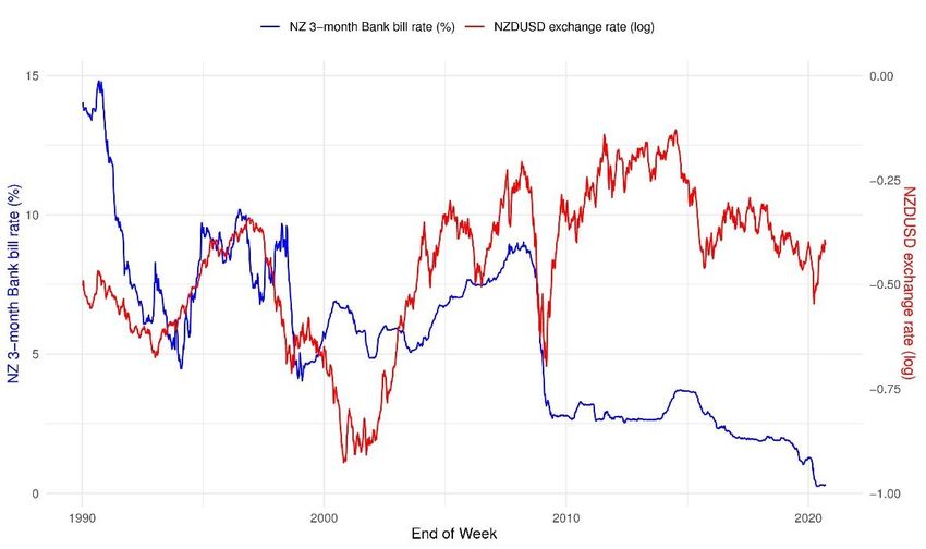
impact on the New Zealand interest rate (stock market), or ∗ = ∗ = 0.2 This assumption
will be relaxed later. Without further assumptions, the structural model in equation (11) is
unidentified. There are 17 parameters to be estimated, including 12 unknown parameters in the
matrix A and 5 diagonal elements in the covariance matrix D of the structural shocks while I
have only 15 known unique elements in the (5 x 5) variance-covariance matrix of the reduced-
form residuals. To exactly identify the model, one needs at least two more equality restrictions.
In this study, I proceed with the Bayesian approach by following Baumeister and Hamilton
(2015), specifying a full prior distribution rather than just sign and zero restrictions for the
unknown structural parameters to get a set identification. In particular, the prior information is
imposed on the elements in the matrix A, not the inverse matrix ( −1 ). I will discuss the chosen
priors in more detail in the next section.

 3.2. Data description

The “raw” data includes the US 3-month Treasury bill rate, the S&P 500 index, the New
Zealand 3-month Bank bill rate, the NZSE index, and the nominal bilateral exchange rate of
NZD against the USD; all in daily frequency. The sample covers the period from 03/01/1999,
when data on the NZSE series started being available, to 18/09/2020. I use weekly data based
on the final trading day of the week to avoid the different daily timestamps across the markets.
I believe that data of higher frequency (such as daily) contain too much noise whereas data of
lower frequency (such as monthly or quarterly) may mute too many variations in stock prices
and exchange rates. Appendix Table A.1 describes data sources in more detail.

For monetary policy reference rates, as the market rates are longer and are more subject to
change than the target rates, I choose the US 3-month Treasury bill rate and New Zealand 3-
month Bank bill rate instead of the Federal Funds rate and New Zealand Official Cash rate.
The left panel in Figure 1 shows that the target rates are relatively stable, especially the New
Zealand Official Cash rate, compared to the market rates. For example, the Official Cash rate
was fixed at 2.5% for almost three years from the week ended on 18/03/2011 to 07/03/2014.
As the market rates appear to co-move strongly with the target rates (the Fed Funds rate and
the US 3-month Treasury bill rate since 2000 as well as the Official Cash rate and New Zealand
3-month Bank bill rate since 1999), I prefer to estimate the market rates with more variations
contained. The left panel in Figure 1 also shows the positive correlation between the US and

2
 For example, Ehrmann et al. (2011) impose a similar assumption of no international spillover effects across the
US and European stock markets and interest rates.

 11

New Zealand market rates, especially clearly from 2004 to 2014. The correlation is not
discernible before 2004 or after 2014.

The exchange rate is quoted per NZD, indicating that a higher value of exchange rate reflects
NZD appreciation. The right panel in Figure 1 implies the positive correlation of New Zealand
3-month Bank bill rate and the nominal exchange rate (in natural logarithm), i.e., higher interest
rate is associated with higher NZD value. This positive correlation does not imply a causal
relationship between New Zealand monetary policy and exchange rate because the interest rate
may be driven by other factors such as foreign interest rates and economic news that may also
cause the exchange rate to change. Therefore, the crucial task is to ensure the unexpected
interest rate changes to be disentangled from other shocks that jointly drive the movements of
both interest rates and exchange rate.

There are various measures of the share market performance in New Zealand. The most popular
measurements are the S&P/NZX family of indices. Among the available proxies, I collect data
on the following: S&P50NZ, NZSE10, NZSEMC, NZSESC, and NZSE; all in nominal NZD.
The S&P50NZ index measures the performance of the 50 largest index-eligible stocks listed
on the NZX Main Board by float-adjusted market capitalization. The S&P50NZ data started
from 29/12/2000 and is widely considered as New Zealand’s pre-eminent benchmark stock
price index. The NZSE10 measures the performance of the 10 largest New Zealand listed
companies within the S&P50NZ index. The NZSEMC measures the performance of New
Zealand’s core mid-cap equity market, covering the constituents of the S&P50NZ index but
excluding those that are also constituents of the NZSE10 index. The NZSESC index is designed
to measure the performance of New Zealand’s smaller listed companies that are not covered in
the S&P50NZ index. The NZSE index is considered as the total market indicator for the New
Zealand equity market, comprising all eligible securities quoted on the NZX Main Board. Apart
from those S&P/NZX indices, there is also the MSCI New Zealand index (MSCINZ), which
is designed to measure the performance of the large and mid-cap segments of the New Zealand
market. The MSCINZ index covers 7 constituents, approximately accounting for 85% of the
free float-adjusted market capitalization in New Zealand. The left panel in Figure 2 plots the
natural logarithms of New Zealand stock prices, implying several common trends in their
variations: all indices increase until the global financial crisis and recover afterward before
entering another declining phase in early 2020 due to the Covid-19 pandemic. Among those
indices, the NZSE series is a composite index based on the prices of stocks excluding
dividends, not a total return stock index. Other S&P/NZX series such as S&P50NZ, NZSE10,

 12

NZSEMC, and NZSESC as well as the MSCINZ index are size-and-style stock indices by
including the stock prices of specific groups of constituents. Despite so-called the benchmark
index, the S&P50NZ series is the shortest among the S&P/NZX family indices with available
since 2000. While these S&P/NZX indices are strongly correlated, I use the NZSE index for
estimation for a longer sample (from 1990 after merging with other variables), which is also in
line with the S&P 500 series used to proxy the US stock market performance. In the right panel
in Figure 2, I plot the S&P 500 and the NZSE indices, all in natural logarithm. I find that the
two stock price indices increase over the 1990-2020 period though their growth rates do not
resemble all the time.

 3.3. Unit root tests and optimal lag length

I conduct multiple unit root tests including Augmented Dickey–Fuller (ADF) test, Phillips–
Perron (PP) test, Kwiatkowski–Phillips–Schmidt–Shin (KPSS) test, and Zivot & Andrews
(ZA) test for stationary testing of the variables. The null hypotheses are different across those
tests. In the ADF and PP tests, the null hypothesis of non-stationarity, i.e. series has a unit root,
is tested against the alternative hypothesis of stationarity. By contrast, in the KPSS test, the
null hypothesis of stationarity is tested against the alternative hypothesis of non-stationarity.
Rejection of the null hypotheses in the ADF and the PP tests, and rejection of the alternative
hypothesis in the KPSS test indicate the series is stationary. In the ZA test, the null hypothesis
is that series has a unit root with a structural break(s) and the alternative hypothesis is that
series is stationary with a break(s). Rejection of the null hypothesis in the ZA test indicates the
series is stationary with a break(s). However, the ZA test can suggest only one break in one
test. I consider all possible cases by including either constant or time trend or both in each test.
Table 1 briefly reports the unit root test results at 5% significance level for five series (interest
rates in percent, stock prices, and exchange rate in natural logarithm), showing whether the
tested series is stationary (I(0)) or non-stationary (I(1)). Detailed results are provided in
Appendix Table A.2.

Table 1 conclusively suggests at 5% level of significance that, the four series including New
Zealand 3-month Bank bill rate, and logs of the S&P 500 index, the NZSE index, and NZD
exchange rate are non-stationary in levels and stationary in first-differences. The only
inconclusive case is the US 3-month Treasury bill rate, which is suggested to be stationary in
the ADF and the PP tests with a time trend included but non-stationary in other tests. Because
all four unit root tests suggest that the US 3-month Treasury bill rate is stationary in first-

 13

difference, I include the first-differences of the US and New Zealand market rates as well as
the log-differences of the US and New Zealand stock price indices and NZD exchange rate in
the estimation.

Next, I check the optimal lag lengths based on the Akaike Information criterion (AIC), the
Hannan Quinn criterion (HQ), the Schwarz criterion (SC), and the Final Prediction Error
criterion (FPE). The AIC and the FPE suggest a similar lag length of 19 while the HQ suggests
4 and the SC suggests 1 as the optimal. Because of the inconsistency of the optimal lags
suggested across those criteria, I proceed with 8 lags for the weekly data.

 3.4. Priors for the structural parameters

I follow Baumeister and Hamilton (2015, 2018) by assigning t-distributions with 3 degrees of
freedom as priors for 12 unknown parameters in the structural matrix A. I will specify the prior
modes, scales, and sign restrictions where possible and intuitive to the literature. All of the
chosen prior modes, except for the effect of exchange rate on New Zealand stock price ( ),
are from Ehrmann et al. (2005). As mentioned in Section 1, their paper studies the financial
transmission between short-term interest rates, bond yields, and equity returns, and exchange
rate within and across the US and the euro area. The reasons I chose that paper as an index of
the prior modes are: they use the ITH approach to report the contemporaneous coefficients in
the structural matrix A, not the inverse matrix −1 ; and they estimate the changes instead of
the levels of variables as reported in the Ehrmann et al. (2011) version. The prior modes are
the average of their estimated coefficients for the US and the euro markets. For example, the
prior mode 0.006 for the effect of stock prices on interest rates ( , ∗ ) are average of their
reported estimators 0.0113 and 0.001. Column 3 in Table 2 provides the prior modes for 12
contemporaneous parameters.

Ehrmann et al. (2005) also report a postive impact of exchange rate on stock price, i.e., a 1%
euro appreciation against USD is associated with a 0.5766% increase in the S&P Euro index.
The S&P 500 index is irresponsive to exchange rate movements, however. For a small open
export-driven economy such as New Zealand, I initially expect instead a negative correlation
as exchange rate appreciation more likely damages export and possibly the stock prices. It is,
however, inconclusive because the impact also depends on the share of export-oriented
constituents in the stock market. Figure 3 plots the NZSE index and NZD exchange rate,
revealing their positive correlation from 1990 to 2015 though their correlation appears to be
reversed since then. To approximately quantify the contemporaneous impact of NZD exchange

 14

rate on the NZSE index ( ), I simply conduct simple OLS estimations which also control for
the dynamic effects of both exchange rate and stock price as follows3

 ∆ = 0 + 1 + 2 + ∑ =1 ∆ − + ∑ =0 ∆ − + (12)

, where ∆LNZSE and ∆LNZDUSD are the log-differences of the NZSE and NZD exchange rate
against the USD. The unit root tests (including the ADF, the PP, the KPSS, and the ZA tests)
suggest that the two series LNZSE and LNZDUSD are non-stationary in levels but stationary in
first-differences. I also include t for the time trend and D as a dummy variable to represent the
break dates of LNZSE suggested by the ZA test (either D1 which gets 1 since 19/10/2007 and
0 otherwise, D2 which gets 1 since 28/12/2007 and 0 otherwise, or D3 which gets 1 since
23/12/2011 and 0 otherwise). Also, 0 is a constant and is the error term. As I will assign
the estimated coefficient as the prior mode of ’s t-distribution, at this stage, I ignore other
determinants and control variables that could affect the NZD exchange rate and the NZSE
index. In the summation terms, p and q are the optimal lag structure, chosen by the AIC. While
the Bayesian Information criterion (BIC) suggests the same lag structure of (2,1) for p and q
for all cases, the AIC suggests the lag structure of (6,2) if including time trend and a dummy
either D1 or D2, and (6,1) if including time trend and D3. Although I prefer the BIC as a
consistent-model selector, I also do not want to under-fit my model, and thus I proceed with
the lag structures chosen by the AIC. The coefficient of interest is 0. Apart from the three OLS
estimations controlling for different suggested structural breaks, I also conduct an OLS
estimation excluding both time trend and dummy variable. The full results are presented in
detail in Appendix Table A.3. In any case, the contemporaneous coefficients are very close,
ranging from 0.21 to 0.218 and all significant at 1% level. As leaving other determinants aside,
the estimators implies a positive association between the NZSE index and the exchange rate,
i.e. 1% appreciation of NZD is associated with approximately 0.2% increase of the stock price,

3
 See Bahmani-Oskooee and Saha (2015) for an extensive review of the studies on the relations between stock
prices and exchange rate. Existing studies either use univariate models or control for other determinants of stock
prices and exchange rate. In any case of using either linear or non-linear models, most of the studies find no or
weak evidence on the long-run equilibrium of the stock prices – exchange rate nexus. Specifically for New
Zealand, Obben, Pech, and Shakur (2006) use the weekly data (average of daily data) of the NZSE index and
disaggregated New Zealand exchange rates (against the USD, the Australian dollar, the British pound, and the
euro) with a cointegrating VAR approach and find ambiguous evidence of the long-run relationship between stock
price and exchange rates. In their equation of the USD/NZD exchange rate, the error correction terms, despite
being negative, are not significant at 5% significance level, indicating no long-run equilibrium exists between
these variables. The short-term coefficients of USD/NZD exchange rate, despite being positive, which implies
that the NZD appreciation is associated with New Zealand stock price increases, are not significant either. No
contemporaneous coefficients are reported in Obben et al. (2006)’s study. Therefore, we estimate equation (12)
using OLS, including both contemporaneous for prior mode and the lagged variables to control for the dynamic
effects.

 15

rather than a causal relationship. I will assign 0.2 as the prior mode of and discuss more this
“positive” impact in Section 4 after achieving posterior distributions and impulse responses.

Next, I impose sign restrictions on the structural parameters, reflecting the interactions between
stock markets, monetary policies, and exchange rate. First, higher stock prices are often
associated with economic booms and inflation, and interest rate is expected to increase to
stabilize inflation, I assume a positive impact of stock prices on interest rates. This assumption
is consistent with the central banks’ mandate. Vice versa, I follow the literature to assume a
negative effect of unexpected interest rate changes on stock prices. For example, Matheson and
Stavrev (2014) impose similar sign restrictions in their bivariate SVAR to examine the US
financial market responses following the Federal Reserve’s taper talk on 22/05/2013 by
disentangling the unexpected monetary shocks from economic news shocks. The intuition is
that a positive economic news shock leads to higher stock prices and a higher interest rate to
stabilize inflation whereas an unexpected tighter monetary policy leads to a higher interest rate
and lower stock prices. Using daily data of 01/2003-06/2014, they find that the immediate rise
in the 10-year Treasury bond yields following the May 22 taper talk is mainly driven by
monetary policy shocks while the effects of positive news shocks become more prominent
during the subsequent months. I also assume a negative effect of exchange rate on monetary
policy, i.e., exchange rate appreciation likely lowers interest rate. Although the positive
correlation between exchange rate and stock price in New Zealand from the OLS estimations
is in line with Ehrmann et al. (2005)’ results, the findings on the impact are not conclusive in
the literature. On the one hand, exchange rate appreciation can curtail exports, profits, and stock
prices of export-oriented companies. On the other hand, appreciation decreases costs of
imported inputs, lowers the production costs of non-exporting firms, hence increases their
profits and stock prices. For this reason, the effect of NZD exchange rate on New Zealand stock
price is left unrestricted. Additionally, despite the positive (negative) prior modes imposed on
the effects of New Zealand (the US) interest rate and stock price on NZD exchange rate, I also
leave their signs unrestricted for more possible posteriors to be achieved. Although the sign
restrictions imposed in traditional SVAR, i.e., sign and exclusion restrictions, are based on the
reasonable belief of the researchers on certain impacts, they restrict the set of identification. In
addition, I agree with Baumeister and Hamilton (2015, 2018)’ criticism on the sign restriction
approach which implicitly assumes that the influence of the priors on posterior will vanish
asymptotically. Those impacts of key interest are left unrestricted in this chapter to allow more
effect scenarios to be obtained. By disclosing the prior information, I am transparent about the

 16

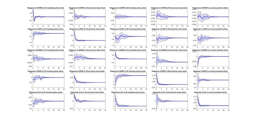
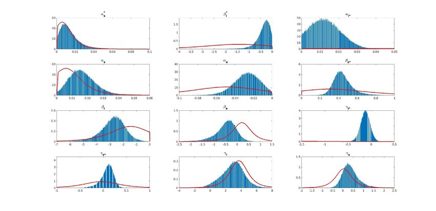
effect of the imposed priors on the posterior distributions and impulse responses. Lastly, I
impose positive sign restrictions on the effects of the US interest rate (stock market) on New
Zealand interest rate (stock market) as those indicators in a small open economy such as New
Zealand will tend to follow the US markets.

Once prior modes and degrees of freedom are chosen, the prior scales determine the prior
width. I choose the scales reasonably so that they meet the sign restrictions accordingly and
more importantly, they are consistent with the previous studies. For instance, the prior for 
and ∗ – the effects of stock prices on interest rates – allows a large probability of 70.46% for
them to be positive, also covering the estimator of 0.021 found by Rigobon and Sack (2004).
For the effect of interest rates on stock prices, I allow a probability of 78.03% for the estimated
parameters and ∗ to be negative, covering other existing estimators of -7.19 and -6.81 found
by Rigobon and Sack (2003), and of -4.68 by Bernanke and Kuttner (2005). Wang and Mayes
(2012)’s estimators for the effects of New Zealand and Australia monetary policy shocks on
stock prices (-3.694 for New Zealand and -1.127 for Australia) using event-study approach are
also included in the prior distributions of and ∗ . For other parameters with unrestricted
signs such as , the prior implies a possibility of 32.57% for a negative impact, i.e., NZD
exchange rate appreciation drives New Zealand stock price to decrease, and 67.43% for a
positive impact. This chosen prior of includes the Ehrmann et al. (2005)’ estimator of
0.5766. For and ∗ , the chosen priors assign a very large probability of 97.3% for ( ∗ ) to
be positive (negative). The prior distribution of is in line with existing estimators in the
literature, including the coefficients of from 2 to 3 found by Zettelmeyer (2004), of
approximately 1.4 by Kearns and Manners (2006), and of 2 by Rosa (2011). By contrast, the
priors imposed on ( ∗ ) imply an equal probability of about 53.58% for them to be positive
(negative).

4. Results

Figure 4 plots prior distributions (solid red curves) and posterior distributions (blue histograms)
for the short-run effects (structural parameters). The key interest is , i.e., the
contemporaneous effect of New Zealand interest rate on NZD exchange rate against the USD,
about which the historical data slightly revises my beliefs as the prior and posterior
distributions are very similar. Despite being sign-unrestricted, the prior and posterior
distributions strongly imply that, following an increase in New Zealand short-term interest rate,
the NZD exchange rate appreciates immediately on impact. I also find it less likely to revise

 17

my belief about the effect of the domestic stock price on short-term interest rate in the US ( ∗ )
but more likely to revise for the New Zealand market ( ) as the posterior distribution for New
Zealand is narrower than the prior distribution. The prior and posterior distributions of – the
contemporaneous effect of New Zealand stock price on NZD exchange rate – also resemble.
However, my beliefs about other short-run effects are revised far more strongly when the
posterior distributions are typically narrower than the prior distributions. The historical data
favors a lower (larger) range for the effect of New Zealand (US) interest rate on stock price.
The data also supports a smaller impact of NZD exchange rate on New Zealand short-term
interest rate ( ) compared to the chosen prior. The posterior distribution of foreign interest
rate’s impact on exchange rate ( ∗ ), while being unrestricted, is far narrower than the prior,
favoring a much smaller effect which is quite close to zero. The data also revises my beliefs
about the effect of NZD exchange rate on New Zealand stock price ( ), with posterior
distribution favouring the negative impact, and the effect of the US stock price on NZD
exchange rate ( ∗ ), with posterior distribution favouring the positive impact. For the
international spillover effects within the same asset class, the data supports a stronger co-
movement of stock prices ( ∗ ) but a smaller for short-term interest rates ( ∗ ).

The median posterior values for the impulse response functions are shown as the solid lines in
Figure 5, along with the 68% and 95% credibility sets. To a 1% unexpected increase in New
Zealand short-term interest rate, I find that the NZD appreciates immediately by 1.51% on
impact. The shaded 68% credibility regions exclude zero, strengthening my belief about the
contemporaneous effect of monetary policy tightening on exchange rate appreciation. The 95%
credibility regions include zero, however. As soon as the interest rate falls back to the initial
level, exchange rate gradually depreciates to its original level. The posterior median of the
direct impact (1.51) is close to other existing findings for New Zealand, such as 1.8–2 found
by Kearns and Manners (2006) but much far from the prior mode (3.698) taken from Ehrmann
et al. (2005).

Most of the other contemporaneous effects are as expected including increasing interest rates
dampen stock prices, New Zealand short-term interest rate (stock price) co-moves positively
with the US interest rate (stock price), a positive US monetary policy shock leads to NZD
depreciation, the US short-term interest rate responds positively to the US economic news
shock (the evidence for New Zealand is weak as the 68% credibility set includes zero), and the
New Zealand interest rate increases in response to a positive currency premium shock. Despite
the zero restrictions on the international spillover effects across asset markets, a higher US

 18

interest rate does cause New Zealand stock price to decrease for two weeks following the shock.
The US stock price has no impact on New Zealand interest rate, however. Interestingly, I find
that a positive economic news shock either in Zealand or in the US leads NZD value to increase
immediately. Last but not least, the results show a negative response of New Zealand stock
price to a positive currency premium shock despite the chosen prior of a positive impact.
However, the impact is overall uncertain because the 68% credibility set of the direct response
of New Zealand stock price to a currency premium shock also contains zero.

Figure 6 plots the median posterior values of cumulative impulse responses. The results show
that the NZD exchange rate keeps appreciating persistently in response to a positive monetary
policy shock: the 6-month accumulated response to a 1% increase in short-term interest rate is
approximately 3.5% and there is no signal of “delay overshooting” over 6 months after the
shock. I also expand the horizon up to one year (52 weeks) following the shock and find very
similar responses of NZD exchange rate: the one-year accumulated appreciation of NZD
exchange rate remains at 3.5%. The results are partly consistent with many existing studies that
find contradict evidence to the UIP theory, which predicts subsequent exchange rate
depreciations following an initial appreciation after a monetary policy contraction. Again, the
findings on the effect of interest rate shocks on exchange rate are largely controversial in the
empirical literature. Some studies, such as Sims (1992) show that the exchange rate depreciates
after monetary tightening, which is the so-called exchange rate puzzle. Most of the other
studies, for example, Cushman and Zha (1997), Kim and Roubini (2000), Kim (2005), as well
as Kim and Lim (2018) report the evidence supporting the “delay overshooting” phenomenon
with the delay lasting shortly, for example at best 6 months found by Kim and Lim (2018).
Scholl and Uhlig (2008), however, document the more prolonged delay from one to three years
before exchange rate starts to depreciate. Various explanations for the failure of the UIP theory
have been discussed. One of them focuses on the invalidity of the two fundamental behavioral
assumptions of the UIP theory in the data: market participants are risk-neutral and they have
rational expectations about future exchange rate movements. If market participants are not risk-
neutral, they will require a risk premium to hold foreign assets over domestic assets. In a recent
paper, Granziera and Sihvonen (2020) relax the second assumption by allowing agents to have
sticky expectations about short-term rates and illustrate that the increase in short-term rate
forecast with sticky expectation occurs with a lag. Because of sticky expectations, agents have
gradually updated their expectations about the short-term rates, the home currency keeps
appreciating. This explains the failure of the UIP theory.

 19

In addition, the results of cumulative impulse responses using the 68% credibility regions
suggest the persistent impacts of short-term interest rates on stock prices and vice versa, of the
US interest rate (stock price) on New Zealand interest rate (stock price), of the US interest rate
on NZD exchange rate, of New Zealand stock price on NZD exchange rate, and of NZD
exchange rate on New Zealand short-term rate. The persistent appreciation of NZD to a positive
economic news shock in the US and the decrease of US stock price to a positive economic
news shock in New Zealand, however, are unexplainable.

Table 3 reports the US and New Zealand variables’ median variance shares, accumulated over
6 months, explained by the monetary policy shocks, economic news shocks, and currency
premium shocks. The results show that New Zealand monetary policy shock plays a very
modest role in explaining the variance of NZD exchange rate (2.62%), which is very close to
Karim et al. (2007)’ estimate of 2.92% (for 4-quarter forecast errors). The largest variance
share of NZD exchange rate is explained by currency premium shocks (75.84%), followed by
New Zealand economics news shocks (11.89%), and the US economic news shocks (9.45%).
For other variables for New Zealand, I find that currency premium shocks can explain 7.32%
of the variance of the short-term interest rate while the contributions of the US monetary policy
and economic news shocks are very small (about 1%). However, the US economic news shocks
can explain up to 17.3% of the variations of the New Zealand stock price, followed by New
Zealand monetary policy shocks (7.97%) and currency premium shocks (6.75%). As expected,
the shocks to New Zealand monetary policy, economic news, and NZD exchange rate attribute
very little to the variances of the US variables.

5. Robustness check

In this section, I cross-check the baseline results by relaxing several restrictions. One of the
assumptions in the benchmark model restricts the international cross-market spillover effects.
This restriction, despite being intuitive and similar to Ehrmann et al. (2011) that assume no
spillover effects across the US and European stock markets and interest rates, could be relaxed
to allow the possible cross-market effects of the US stock price (interest rate) on New Zealand
interest rate (stock price). In a sequent check, I also relax the sign restriction on the effect of
exchange rate on interest rate ( ). While the baseline model supports a negative relationship
between exchange rate and interest rate - domestic currency appreciation is associated with
lower interest rate – this additional check instead allows an opposite scenario to happen when
the currency appreciation caused by a positive risk premium may be associated with a higher

 20

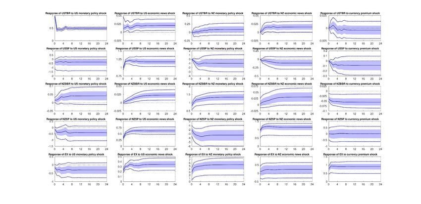
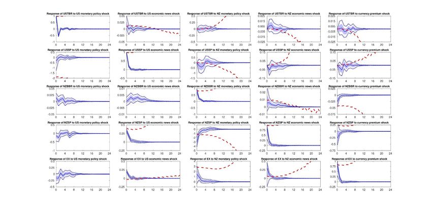
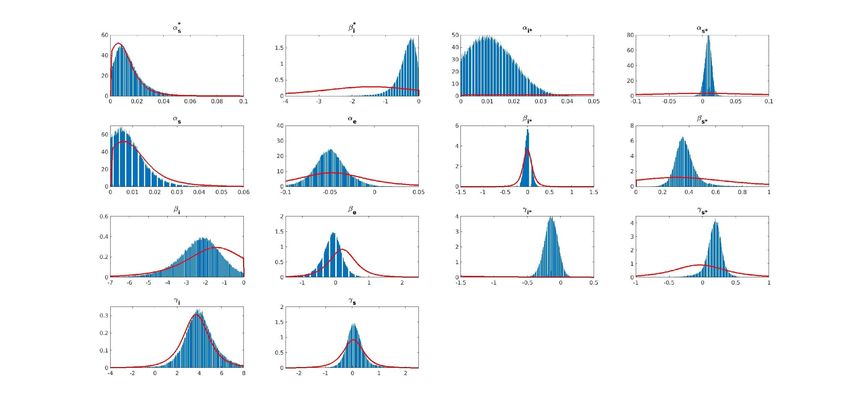
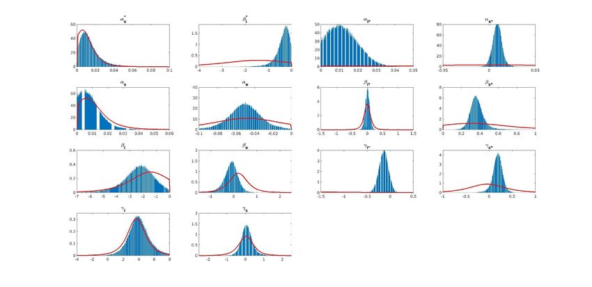
interest rate, i.e. investors switch to riskier assets rather than government bonds. As stock prices
could also increase in that scenario, currency appreciation still leads to a comovement of stock
price and interest rate. In any case, the main findings remain – a higher interest rate leads NZD
to appreciate immediately and even stay stronger in the long-run. The sub-sections below
describe the results in more detail.

 5.1. International cross-market effects

First, to allow the New Zealand interest rate (stock price) to respond to the US stock price
(interest rate), I impose a tight t-distribution with 3 degrees of freedom, prior mode of zero,
prior scale of 0.1, and non-restricted sign on ∗ - direct effect of the US stock price on the
New Zealand interest rate and ∗ - direct effect of the US interest rate on the New Zealand
stock price. The results are provided in Appendix Figures A.1 - A.3 for prior and posterior
distributions, impulse responses, and cumulative impulse responses. Figure A.1 includes the
prior and posterior distributions of 14 contemporaneous parameters: the posterior distributions
of 12 existing parameters are very similar to the baseline results and those of the two newly
added parameters ( ∗ and ∗ ) appear very sharply peaked, even more around zero for ∗ . In
Figure A.2 for the impulse responses, New Zealand stock price decreases as a response to a
higher US interest rate (significantly at 68% credibility set but insignificantly at 95% credibility
set). New Zealand interest rate, however, shows insignificant responses to the US stock price
changes. This result makes sense as New Zealand monetary policy tends to stabilize the
domestic inflation rather than reflects the stock price changes in the US market. The negative
responses of the New Zealand stock prices to the US monetary policy, however, are intuitive
as reflecting the comovement of stock prices across the two markets. Relaxing the cross-market
spillover effects also leaves the responses of other variables unchanged, except a larger
appreciation of NZD (3% in the short-run and 5.4% in the long-run approximately) due to a
1% increase in New Zealand interest rate, which is statistically significant at 68% credibility
set (Figures A.2 – A.3).

 5.2. Effect of exchange rate on interest rate

This second check relaxes both international cross-market spillover effects and the sign
restriction on the impact of exchange rate on interest rate. Specifically, apart from imposing
the tight t-distribution for ∗ and ∗ as in Section 5.1, the parameter now has an
unrestricted sign. The results are included in Appendix Figures A.4 - A.6. Although the
posterior distribution of now includes positive values due to the sign relaxation, a large

 21