Material flows and GHG emissions from housing stock evolution in US counties, 2020-60
←
→
Page content transcription
If your browser does not render page correctly, please read the page content below
A correction article relating to this paper has been published and can be found at http://journal-buildingscities.org/articles/10.5334/bc.150/
A correction article relating to this paper has been published and can be found at http://journal-buildingscities.org/articles/10.5334/bc.150/
Material flows and GHG
emissions from housing
stock evolution in US
counties, 2020–60 RESEARCH
PETER BERRILL
EDGAR G. HERTWICH
*Author affiliations can be found in the back matter of this article
ABSTRACT CORRESPONDING AUTHOR:
Peter Berrill
The evolution of housing stocks determines demand for construction materials and energy, Center for Industrial Ecology,
and associated emissions of greenhouse gasses (GHGs). The contribution of construction to Yale University, New Haven,
building life-cycle emissions is growing as buildings become more energy efficient and the CT, US
energy supply decarbonizes. A housing stock model is developed for counties in the United peter.berrill@yale.edu
States using dynamic vacancy rates which endogenously influence stock out- and inflows.
Stocks of three house types and 10 construction cohorts are projected for all contiguous
US counties for the period 2020–60. Inflows and outflows of construction materials KEYWORDS:
are then estimated along with GHG emissions associated with material production and building stock; construction
construction activities in scenarios defined by stock turnover rates, population share by demand; floor area; embodied
house type, and floor area characteristics of new houses. The results provide new insights GHG emissions; housing;
material flow; resource
into the drivers of construction-related emissions at local and national levels, and identify
efficiency; vacancy; US
opportunities for their reduction. Demolition material flows grow in relation to construction
material flows over the analysis period. Increasing the stock turnover rate increases future
TO CITE THIS ARTICLE:
floor area per person, material requirements, and emissions from construction. Scenarios
Berrill, P., & Hertwich, E. G.
with reduced floor area and more multifamily homes in new construction have lower floor (2021). Material flows and
area growth, material requirements, and emissions from construction. GHG emissions from housing
stock evolution in US counties,
POLICY RELEVANCE 2020–60. Buildings and Cities,
2(1), pp. 599–617. DOI: https://
Housing construction constitutes an important share of annual residential GHG emissions doi.org/10.5334/bc.126
in the US. The characteristics of new construction also influence residential energy use
over longer time periods. Increasing the share of multifamily housing in construction and
reducing the average size of new single-family homes by eliminating very large homes are
two strategies that can reliably and substantially reduce the environmental burdens of
new construction. These same strategies would limit or, if combined, reverse the growth
of residential floor area per person, enabling reductions of energy-related emissions.
Policymakers can therefore reduce residential sector emissions in the short and long
terms by encouraging the supply of multifamily homes and smaller housing typologies,
and limiting construction of large homes.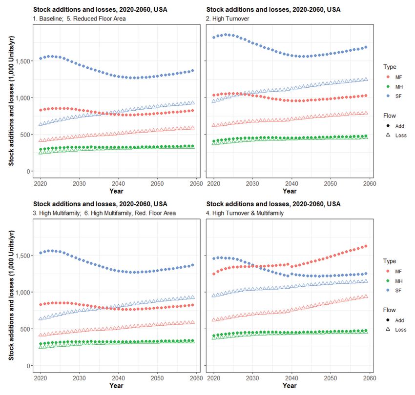
1. INTRODUCTION                                                                                        Berrill & Hertwich
                                                                                                       Buildings and Cities
                                                                                                                              600

                                                                                                       DOI: 10.5334/bc.126
Buildings are a major contributor to anthropogenic greenhouse gas (GHG) emissions. The extent
to which emissions can be reduced from both the construction and operation of buildings will
play a key role in determining the feasibility of achieving ambitious climate change mitigation
targets (Krausmann et al. 2020). As building stocks evolve through construction and demolition,
they require new materials, produce construction and demolition waste, and generate ‘embodied’
GHG emissions from material production and construction activities. Evolution of building stocks
can reduce energy-related emissions, as newer buildings replace older, less efficient buildings.
However, embodied emissions are growing more important as buildings become more efficient
and as the energy supply becomes less carbon intensive (Röck et al. 2020). The need to reduce
embodied emissions becomes clearer when considering the limited remaining timeframe and
carbon budgets for keeping climate change within 1.5–2.0°C warming. Building stock models are
widely used to estimate building and material stocks and flows (Augiseau & Barles 2017; Lanau et
al. 2019), energy and GHG emissions from building energy use (Langevin et al. 2020), and, in limited
cases, GHG emissions from both building construction and energy use (Pauliuk et al. 2021; Pauliuk
& Heeren 2020). The role of vacancies, and their influence on building construction, demolition,
and material flows, is beginning to receive more attention in building stock models, particularly
in regions with declining population and growing vacancy rates (Deilmann et al. 2009; Wuyts et
al. 2020). Areas with high vacancy rates tend to have lower demand for new construction (Volk
et al. 2019), while areas with low vacancy rates have higher construction demand (Zabel 2016).
Improved modeling of construction and demolition considering local population growth and
vacancy rates can facilitate more reliable construction and demolition material flow estimates at
local levels (Schiller et al. 2017b), where reuse of bulky materials is more feasible.

This paper describes the development and application of a housing stock model for 3108 US
counties (excluding counties in Alaska and Hawaii) and projects the evolution of the US housing
stock by county over the period 2020–60. Dynamic, county-specific vacancy rates are incorporated
in the model, and historical survey data are used to estimate region- and house type-specific
‘natural vacancy rates.’ Drawing on observed and natural vacancy rates in each timestep, novel
approaches are applied to modeling stock additions and losses. The geographic resolution of
US counties enables the estimation of housing stock evolution and material flows at a local
level. Model results can thus demonstrate the potential (or lack thereof) for local circular reuse
of construction materials. Housing stock and material flows, GHG emissions associated with
new construction, and the progression of residential floor space per person are illustrated for six
scenarios. The scenarios investigate the material demand and embodied GHG implications of
different strategies with potential to reduce energy and embodied emissions in US housing.

2. REPRESENTATION OF VACANCY IN HOUSING STOCK MODELS
Research on housing markets in economics has yielded support for the existence of natural vacancy
rates, which can generally be understood as the result of a housing search process by households
with varying preferences within a heterogenous housing stock, and can vary by region (Rosen &
Smith 1983; Wheaton 1990; Zabel 2016). Hwang & Quigley (2006), the first to include vacancies as
an input to economic housing supply models, showed that lower vacancy rates are likely to persist
in more heavily regulated housing markets. Zabel (2016) specified a model to estimate changes in
housing supply based, in part, on local vacancy rates, and found that vacancy above the natural
rate has a downward effect on new housing construction, while vacancy below the natural rate
has an upward effect on new construction. These studies provide some explanations for non-zero
vacancy rates in housing markets, building on the understanding of vacancy arising from a search
process by mobile populations. They also indicate relationships between regulations, vacancy
rates, and housing supply. Unlike dynamic stock models produced for material flow analyses
(MFAs), however (Lanau et al. 2019), these economic models focus only on housing supply and do
not disaggregate net stock growth into additions and losses.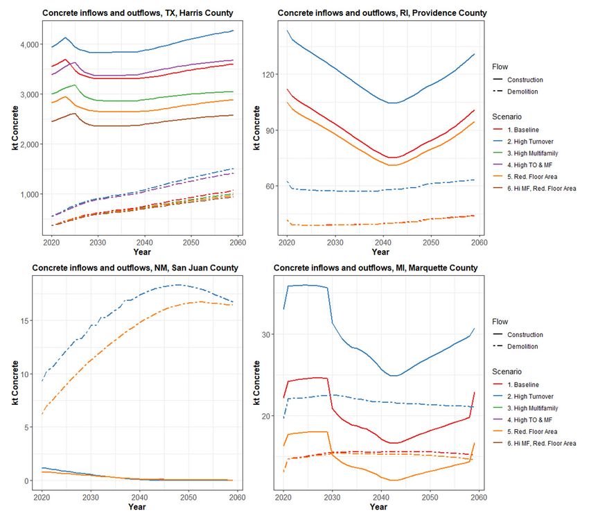
In dynamic building stock models used in industrial ecology and MFA, explicit consideration of Berrill & Hertwich 601
Buildings and Cities
vacancy rates is an emerging practice. Disregarding vacancies can lead to infeasible negative DOI: 10.5334/bc.126
inflows in cases of negative stock growth (due to population decline) (Deetman et al. 2020). This
is largely because housing demolition does not respond to population decline in the same way
that construction responds to population growth (Schiller et al. 2017a). Vásquez et al. (2016)
address this issue by subtracting vacant floor area arising from declines in population from their
estimates of in-use stock, but they do not account for what they call ‘market vacancies.’ Some
models do incorporate explicit consideration of non-static vacancy rates. Deilmann et al. (2009)
generated scenarios describing housing stock evolution in eastern and western Germany to 2050,
highlighting the increase in vacancies that would accompany population decline, unless loss
rates also increased. Roca-Puigròs et al. (2020) use three occupancy states (daily use, temporary
use, and vacant stock) in their description of the Swiss housing stock, although vacancy rates did
not change over time, or play a role in determining stock in- or outflows. Schiller et al. (2017a)
estimate a maximum vacancy threshold to inform their calculation of residential demolition in
Germany. Volk et al. (2019) use vacancy rates for multifamily buildings to approximate vacancy
rates for residential and non-residential buildings in the German state of Baden-Württemberg, and
model vacancy increases in response to reduced demand for new floor area, as well as reduced
replacement of demolished buildings in regions with higher vacancy. These studies exemplify the
evolving treatment of vacancy in building stock models. A prevailing approach to incorporating
vacancy in such models has not yet emerged.
3. DATA AND METHODS
For this study, a bottom-up housing stock model is developed for US counties, classifying housing
stocks by type (single-family, multifamily, manufactured housing; manufactured housing is a form
of single-family, but has very different lifespan, vacancy rate, and material intensity characteristics),
by construction cohort, and by vacancy status (occupied/vacant). The principal data sources used
for model development are longitudinal datasets spanning the period 1985–2017, indicating the
movement of housing units in and out of the housing stock (US Census Bureau 2017b), and the
corresponding American Housing Survey (AHS) microdata (US Census Bureau 2020a). ‘Components
of inventory change’ reports based on these data describe how a substantial portion of housing
units move in and out of the stock from processes other than new construction and demolition
(Eggers & Moumen 2016, 2020). In addition to demolition and disaster, housing stock losses also
arise from houses changing to non-residential uses, becoming damaged or unfit for habitation,
or from (mobile) manufactured homes moving out from the site where they were last surveyed.
In addition to new construction, housing stock additions also occur from conversions from non-
residential to residential use, recovery from temporary losses (including previously uninhabitable
buildings returning to the housing stock), and manufactured homes moving into new sites. In
these surveys and reports, a housing unit is only considered to be part of the total (occupied plus
vacant) housing stock if it is physically fit for habitation, and available for residential use, i.e. not in
use for a non-residential purpose.
Figure 1 shows a schematic diagram of the model inputs and outputs; Table 1 details the variables
and superscripts used in the equations that follow. The housing stock model is defined in equations
(1) to (6) and the accompanying text. For further detail on the results processing, see Section S5
and Figure S11 in the supplemental data online.
The starting point for the model is the calculation of the occupied stock S (measured in housing
units) of each house type in every county for each model year, based on county resident
population P, county population share by house type P%, and average household size HS by house
type (equation 1) (see Table 1 for definitions of each variable and subscript):
S t ,k ,v
0, y
P k , y P%t ,k , y /HS t ,k , y (1)
Population projections for US counties were generated using a blended cohort-change differences
and cohort-change ratios model (Hauer 2019) for five shared socioeconomic pathway (SSP)
scenarios (O’Neill et al. 2017). This study adapts Hauer’s (2019) SSP2 (‘middle of the road’) county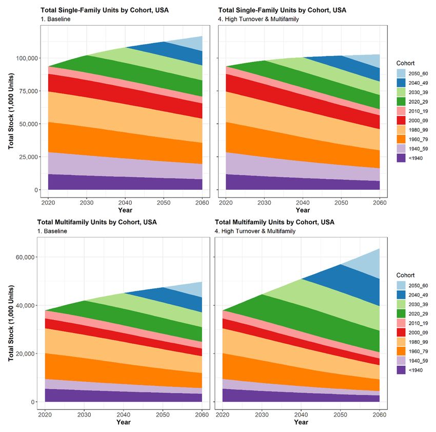
Figure 1: Schematic of inputs
                                                                                           Con./Dem.
                                                                                             % of            Avg. Floor    Material,    and outputs from the housing
       HSM inputs
                                                                                                              Areat,c,k    GHG Int.a
                                                                                           Add.Losst                                    stock model.
                                                                                                                                        Note: Con. = construction;
     Total Populationk
                                                                                                                                        Dem. = demolition;
                                                                    Annual Outflowst,c,k                                                Add. = additions; Loss = losses.
                                               Housing                                                                                  Int. = intensity, referring to
                                                                     Annual Inflowst,c,k          Results Processing
                                                Stock                                                                                   material per unit of floor area
'Natural' Vacancy Ratet,r                       Model                                                                                   (kg/m2), greenhouse gas (GHG)
                                                                      Total Stockt,c,k,v
 Household Sizet,k                                                                                                                      per mass material (kgCO2e/kg),
                                                                     Superscripts:                                                      and the resulting GHG per unit
                                                                     t = house type
                                                                c = construction cohort                                                 floor area (kgCO2e/m2). For
                                                                        k = county
                                                                   r = census region
                                                                                                                                        a description of the results
                                                                  v = vacancy status       Material          GHG from                   processing, see Figure S11 in
                                                                                                            Construction     m2/cap
                                                                     a = archetype         inflows/
                                                                                           outflows                                     the supplemental data online.

 SYMBOL           SUMMARY                                                                             UNIT OF MEASUREMENT/SUPERSCRIPT DETAIL

 S                Housing stock                                                                       Number of housing units

 P                Population                                                                          Persons

 P%               Population share                                                                    (%)

 HS               Household size                                                                      Persons/housing unit

 L                Losses from stock                                                                   Housing units/year

 LR               Loss rate                                                                           Lost housing units/total housing units

 A+OSG            Additions to the stock with positive OSG                                            Housing units/year

 A–OSG            Additions to the stock with negative OSG                                            Housing units/year

 AR               Additions rate                                                                      Added housing units/total housing units

 TSG             Total stock growth                                                                   Total housing units/year

 OSG              Occupied stock growth                                                               Occupied housing units/year

 GF               Growth factor determining the ratio of TSG to vacancy-adjusted OSG                  []

 VF               Vacancy factor (total stock/occupied stock)                                         []

 V                Vacancy rate (vacant stock/total stock)                                             []

 t                Superscript for house type                                                          Three types (single/multi-family, manufactured home)

 c                Superscript for house construction cohort                                           Ten cohorts

 k                Superscript for US county                                                           3108 counties

 v                Superscript for house vacancy status                                                Two levels: 0 = occupied, 1 = vacant

 r                Superscript for US Census region                                                    Nine regions

 y                Superscript for model year                                                          Range covered: 2020–60

population projection to 2060, scaled first to the US Census Bureau mid-range national population                                       Table 1 Housing stock model
projection (US Census Bureau 2017a) (see Figure S1 in the supplemental data online) and again                                           variables and superscripts.
to the actual US resident population on 1 July 2020 (US Census Bureau 2020c), to bring the
projections in line with recent US national population levels and projections. Estimates of future
changes in household size (see Figure S2 in the supplemental data online) are based on data from
McCue (2018), and the same proportional reduction in household size is applied to all house types,
while maintaining the initial differences in household size observed in different counties and house
types. Initial estimates of household size and population share by house type in each county are
derived from one- and five-year population and occupied housing unit estimates for 2019 from
the American Community Survey’s (ACS) tables B25033 and B25127 (US Census Bureau 2021).
This estimation is elaborated further in Section S1.1 in the supplemental data online.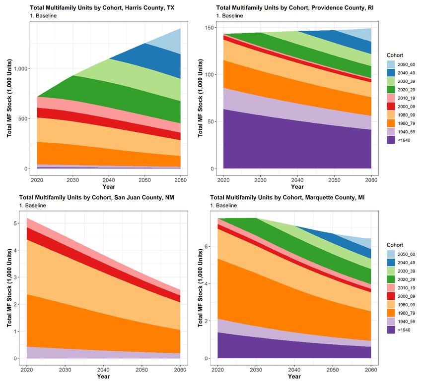
In the second model step, losses are calculated from the housing stock based on annual loss Berrill & Hertwich 603
Buildings and Cities
rates, summarized in Table S1 in the supplemental data online. Loss rates for each age cohort DOI: 10.5334/bc.126
are calculated for each year based on the share of age ranges that exist in each age cohort.
For example, in 2025, some of the houses built between 2000 and 2009 will be in the 0–19-
year age range, while others will be in the 20–59-year age range, and so the loss rate for these
houses will be a weighted average of loss rates for these two age ranges. Total housing losses (L)
are then calculated as the product of total stock (S) by type, cohort, county, and vacancy, and
corresponding loss rates (LR) (equation 2):
t ,c ,k ,v , y
L S t ,c ,k ,v , y LR t ,c ,r ,v , y (2)
By adding an age-related dependency to loss rates, the modeling of decay of existing buildings
combines the ‘lifetime’ and ‘leaching’ approaches described by Roca-Puigròs et al. (2020). The
introduction of vacancy-dependent loss rates is a novelty of this model and motivated by the large
differences in loss rates observed for occupied and vacant units. Vacant units are much more likely
to leave the stock than comparable occupied units (see Table S1 in the supplemental data online).
Next, additions to the stock are calculated with separate approaches employed depending on
whether occupied stock growth (OSG) in a model year is positive or negative. Positive and negative
OSG generally correspond to positive and negative population growth, but reductions in household
size can also generate a positive OSG even in the case of zero or marginally negative population
growth. In most housing stock models, it is assumed that there will be no new additions to the
stock if the occupied stock does not grow. The authors’ reading of AHS data suggests that this
is not necessarily the case. At national and census region levels, positive additions to the stock
occur even in times of negative OSG (see Figure S4 in the supplemental data online). This can be
explained by some demand for new housing existing within a region, even if the occupied stock in
the region as a whole declines. A linear model (see Table S4 in the supplemental data online) is
used to estimate the addition rate (AR ≥ 0) conditional on the OSG rate in cases of negative OSG.
This estimate of AR is then multiplied by the total stock to calculate additions to the stock in cases
of negative OSG, A–OSG (equation 3):
t ,k , y t ,r t ,k , y
A OSG AR S (3)
For cases of positive OSG, annual additions to the stock, A+OSG, are calculated as the sum of total
stock growth (TSG) and losses (L) (equation 4). TSG equals the product of OSG, a ‘natural’ vacancy
factor (VFn), and an estimated stock growth factor (GF), which defines the ratio of actual TSG to
vacancy adjusted OSG (see equation S1 in the supplemental data online).
t ,k , y
A OSGt ,k , y TSGt ,k , y Lt ,k , y (GF VFnt ,r OSGt ,k , y ) Lt ,c ,k ,v , y (4)
c ,v
The natural vacancy factor VFn is defined as the total stock divided by the occupied stock when
vacancy is at the natural level. VFn is equivalent to (1 – Vn)–1, where Vn is the natural vacancy rate.
GF can fluctuate, increasing or decreasing the level of stock growth (and consequently additions
to the stock) in order to move the stock towards the natural vacancy rate. For example, if vacancy
rates are below the natural rate, GF > 1, which will increase additions to the stock and cause the
vacancy rate to increase. If vacancy rates are above the natural rate, GF < 1, reducing additions
to the stock and causing the vacancy rate to decrease. A linear model is specified to estimate GF
as a linear function of changes in the vacancy factor dVF (see Figures S5–S7 in the supplemental
data online) based on historical AHS data (US Census Bureau 2017b, 2020a). The value of GF is
estimated conditional on the change in vacancy factor dVF, assuming that dVF equals half the
difference between the actual vacancy factor and the natural vacancy factor in a given year, i.e.:
y y
dVF 0.5* VFn – VF .
This specification reflects the assumption that in growing stocks, vacancy factors (and vacancy
rates) will tend towards the exogenously determined natural level, with the factor 0.5 preventing
the gap between actual and natural VF from being closed too quickly. If the housing stock is
already at the natural vacancy rate, GF = 1 and TSG is simply the product of VF and OSG.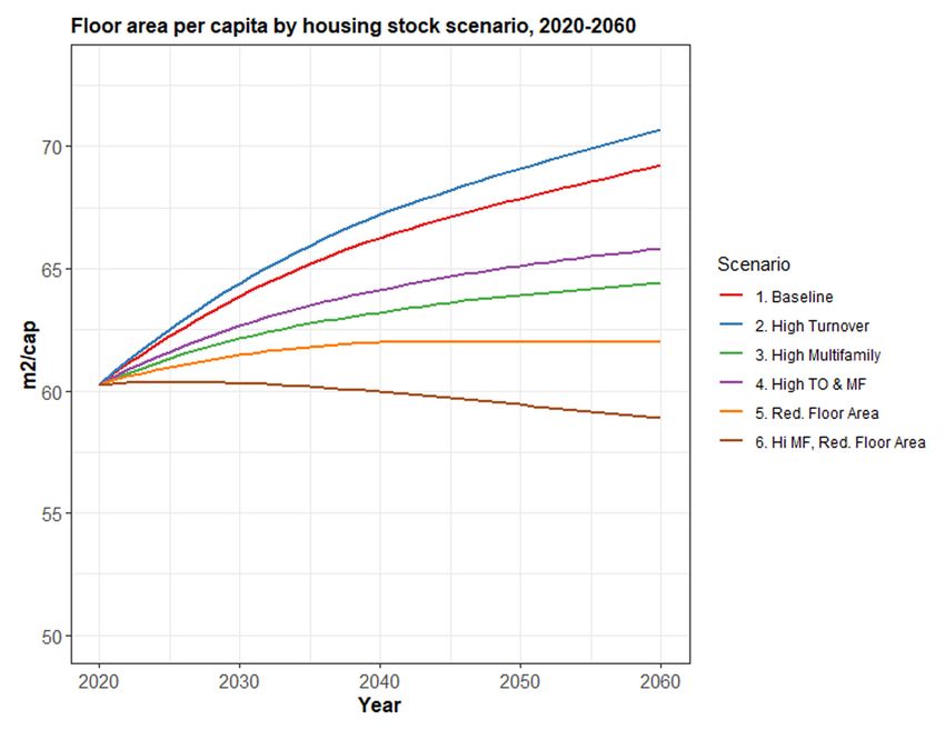
Natural vacancy rates are estimated using the mean vacancy rates for each house type and Berrill & Hertwich 604
Buildings and Cities
census region calculated from AHS data for the period 1985–2019. National vacancy rates average DOI: 10.5334/bc.126
approximately 10%, 15%, and 20% for single-family, multifamily, and manufactured housing,
respectively, with some variation around these levels for different census regions (see Figure S8 in
the supplemental data online). To describe vacancies in the housing stock in 2020, vacancy rates
are calculated by type, cohort, and county using data on occupied and total housing stocks from
ACS tables DP04 and B25127 (US Census Bureau 2021). The total stock by type for the beginning of
year y + 1 is calculated based on the initial stock, additions, and losses in year y (equation 5), and
vacancy factors are then calculated as total stock divided by occupied stock (equation 6):
t ,k , y 1
S S t ,k , y At ,k , y Lt ,k , y (5)
t , y 1
VF S t ,k , y 1 /S t ,k ,v
0, y 1
(6)
In order to calculate material flows associated with additions and losses to the stock, first the
additions and losses are converted into new construction and demolition. The portion of additions
to the stock coming from sources other than new construction varies by region and type, but
additions from new construction tend to be around 85% of total additions (see Table S2 in the
supplemental data online). For demolition, it is assumed that on average 35%, 20%, and 45% of
single-family, multifamily, and manufactured housing losses from stock are due to demolition
or disaster (see Table S3 in the supplemental data online). The resulting estimates of material
in- and outflows are very sensitive to the conversion of additions to new construction, and losses
to demolition, respectively. The percentages of losses from demolition that are adopted here
are slightly higher than historical rates (see Table S3 online), because it is assumed that many
of the houses that leave the stock for reasons other than demolition will likely be demolished
in subsequent years, and therefore actual demolitions in a given year will include demolition of
some ‘hibernating stock’ (houses that left the in-use stock in previous years, which are not picked
up by AHS statistics). Some remaining houses that leave the stock will not be demolished while
materials are still recoverable, leading to ‘dissipative flows’ of building materials which cannot be
recovered (Jelinski et al. 1992).
Estimates of average floor area per house type, cohort, and county are based on floor area
characteristics by core-based statistical areas (CBSA) from the AHS 2017 survey, as incorporated
in the ResStock housing characteristics database (NREL 2020). Details for estimating floor area
characteristics at county resolution are given in Section S2 in the supplemental data online.
Housing characteristics for Hawaii and Alaska are excluded from the ResStock database, and so
the model also excludes these states, which together represent 0.6% of the US housing stock.
In all cases, references to floor area describe ‘useful floor area,’ which excludes basements and
garages. Total occupied floor area is calculated by multiplying the number of occupied housing
units per county by the average floor area per house (see Figure S11 in the supplemental data
online). Combining the occupied floor area data with population estimates, the evolution of floor
area per person (m2/cap) per county and house type is then calculated. Floor area and population
data can then be aggregated to calculate the floor area per person for all house types and/or for
larger geographic units. Calculating floor area per person as a model output contrasts with the
approach in most housing stock models, where floor area per person is an exogenously assumed
model input, reflecting service level (Müller 2006; Pauliuk et al. 2021; Roca-Puigròs et al. 2020). The
approach taken here facilitates the identification of stock characteristics and dynamics that will
influence the future growth of floor area per person, and the identification of strategies than can
be pursued to constrain this growth. Average floor area per house type, cohort, and county are
also used to convert construction and demolition flows from housing units into floor area in- and
outflows (see Figure S11 online).
The Athena Impact Estimator (Athena Sustainable Materials Institute 2020) is used to generate
material intensities for 51 housing archetypes (described in Section S3 in the supplemental data
online), and these are then used to estimate weighted-average material intensities by house
type and county for 48 construction materials. To calculate material-related GHG intensities,
29 material categories are then defined for which GHG emissions/kg of material production are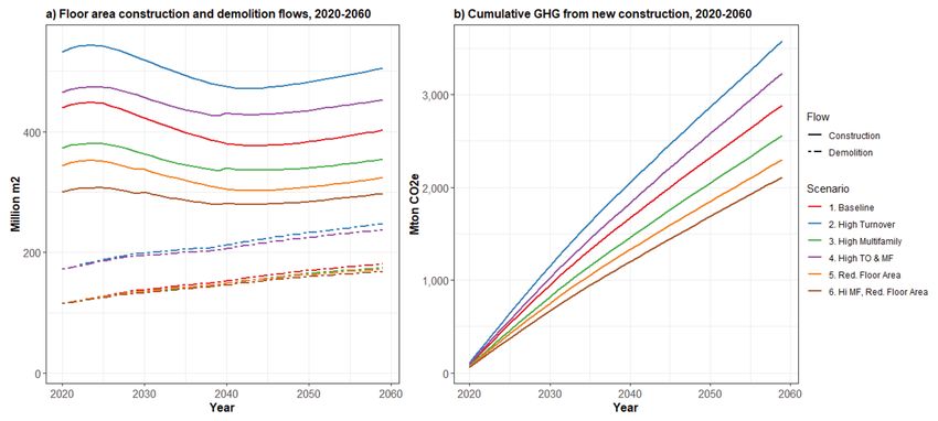
obtained. Material GHG intensities come from a variety of sources including environmental product                  Berrill & Hertwich           605
                                                                                                                   Buildings and Cities
declarations and life-cycle assessment databases (Jones 2019; Wernet et al. 2016). Intensities                     DOI: 10.5334/bc.126
are based on the most recent and US-representative sources where possible. GHG emissions
from construction site transport and energy use are incorporated based on archetype-specific
estimates from Athena, scaled to be more consistent with literature estimates (see Table S6
in the supplemental data online). Archetype characteristics are summarized in Table S5 in the
supplemental data online; the GHG intensity from all materials and construction activities per
floor area is shown in Figures S9 and S10 in the supplemental data online. Avoiding basement
foundations, building multi-storey (for a given floor area), and building without a garage are some
options that exist for reducing GHG emissions from new single-family construction.

Six scenarios of housing stock evolution are generated along dimensions of population share by
house type, housing stock loss rates, and average size of new housing (Table 2). The scenarios
reflect housing stock strategies that may be adopted to reduce direct energy demand, and energy
and embodied emissions. The effects of these scenarios on energy consumption and emissions
are the focus of future research. This paper demonstrates housing and material flows, and related
emissions, for each scenario at a county and national level. In a Baseline scenario, population
share by house type is assumed to remain constant throughout the projection period. In a High
Turnover scenario, the loss rates (see Table S1 in the supplemental data online) are increased by
a factor of 1.5, which is comparable to reducing the average lifetime for all housing by one-third.
In cases of positive OSG, this will directly produce higher stock additions, as described in equation
(4). For negative OSG, the factor of 1.5 is also applied to the additions estimated in equation (3).
In a High Multifamily scenario, the share of the population living in multifamily is increased by
0.25 percentage points (pp)/year in counties where the population grows by at least 5% over
20 years between 2020–40 and 2040–60. The High Turnover & High Multifamily scenario simply
combines the loss rate and population share assumptions of scenarios 2 and 3. In a Reduced Floor
Area scenario, the floor area distributions are redefined so that any new house >279 m2 (3000
square feet) is instead in the range of 186–278 m2 (2000–2999 square feet) (cf. Figure S15 in the
supplemental data online). To put this scenario in the context of recent trends, between 25% and
30% of new single-family houses built in the 2010s were ≥279 m2 (US Census Bureau 2020b). In
order to fit with scenarios in which residential floor area consumption converges to a range of
                                                                                                                   Table 2 Summary description
30–40 m2/cap (Grubler et al. 2018; Hertwich et al. 2020), a 279 m2 house would require seven to                    for six housing stock scenarios.
nine inhabitants. In 2019, houses of ≥279 m2 had on average 3.06 occupants (US Census Bureau                       Multifamily population
2020a). The High Multifamily, Reduced Floor Area scenario combines the population share and                        increases apply only to counties
floor area distribution assumptions of scenarios 3 and 5. With the exception of the Reduced Floor                  where population growth > 5%
Area scenarios (5 and 6), floor area characteristics for new housing in future cohorts are assumed                 over 20 years for the periods
                                                                                                                   2020–40 and 2040–60.
to remain the same as housing built in the 2010s (see Figures S14 and S15 in the supplemental
                                                                                                                   Note: FA = floor area;
data online).
                                                                                                                   pp = percentage points.

 SCENARIO         1                      2                 3                     4                       5                     6
                  BASELINE               HIGH TURNOVER     HIGH                  HIGH                    REDUCED FA            HIGH
                                                           MULTIFAMILY           TURNOVER AND                                  MULTIFAMILY,
                                                                                 MULTIFAMILY                                   REDUCED FA

 Loss rate         Historical rates by   1.5× Historical   Historical rates by   1.5× Historical rates   Historical rates by   Historical rates by
                   region                rates by region   region                by region               region                region

 Multifamily      2020 share by          2020 share by     Increase 0.25         Increase 0.25           2020 share by         Increase 0.25
 population       county                 county            pp/year               pp/year                 county                pp/year

 Floor area        Same as 2010s         Same as 2010s     Same as 2010s         Same as 2010s           No homes > 279        No homes > 279
 distribution,                                                                                           m2                    m2
 new homes

4. RESULTS
4.1 AGGREGATED NATIONAL RESULTS
Figure 2 shows annual additions and losses to the stock, aggregated to the national level, from
2020 to 2060 for the six housing stock scenarios. In all scenarios, additions to the stock are higher
than losses, reflecting continual stock growth. In the High Turnover scenarios, there are much Berrill & Hertwich 606
Buildings and Cities
higher levels of stock losses and additions. In the High Multifamily scenarios, multifamily inflows DOI: 10.5334/bc.126
are substantially higher than in the Baseline, and become higher than single-family additions in
the late 2020s/early 2030s. Because these figures depict flows of housing units and not floor area,
scenarios 1 and 5 are identical, as are scenarios 3 and 6.
Figure 2: Inflows (additions)
and outflows (losses) from
stock for three house types for
each housing stock scenario.
Figure 3 compares the growth of national single- and multifamily stocks in scenarios 1 and 4. From
a 2020 level of 94 million units, the stock of single-family houses grows to 103 million units by
2060 in scenario 4, compared with 117 million units in the baseline scenario 1. The multifamily
stock grows from 38 million units in 2020 to 50 million (scenario 1) or 64 million (scenario 4)
units by 2060. With higher stock turnover, the existing stock declines slightly faster. The pre-1960
housing declines from 27.3% of the total housing stock in 2020 to 14.4% in 2060 in scenarios 1,
3, 5, and 6, or 11.9% in scenarios 2 and 4. These relatively small differences in decline of older
housing demonstrate that even with a considerable increase in demolition rates, more than 10%
of the housing stock in 2060 will be over 100 years old.
Figure 4 shows the implications of the housing stock scenarios for the evolution of national occupied
floor area per person (m2/cap). In the Baseline scenario, steady growth occurs from 60.2 m2/cap
in 2020 to 69.2 m2/cap by 2060. Although declines in average household size play some role, this
growth in m2/cap is primarily because housing built from 2020 onwards is much larger on average
than housing that leaves the stock, which is mostly from the early and mid-1900s (see Figure S14
in the supplemental data online). Speeding up the turnover rate in scenario 2 accelerates this
growth, and floor space per person reaches 70.7 m2/cap by 2060. Due to lower floor area per
person in multifamily housing, increasing the multifamily share in scenario 3 attenuates the
growth in floor area per person, which grows to 64.4 m2/cap by 2060. The Reduced Floor Area
scenario shows floor area per person stabilizing at 62.0 m2/cap from 2040 onwards, while theBerrill & Hertwich 607 Buildings and Cities DOI: 10.5334/bc.126 Figure 3: Evolution of single- and multifamily housing stocks by construction cohort for two scenarios. Figure 4: Occupied floor area per person in each housing stock scenario.
lowest trajectory is achieved by combining high multifamily and reduced floor area (scenario 6),      Berrill & Hertwich          608
                                                                                                      Buildings and Cities
which reduces floor area per person to 58.9 m2/cap by 2060. The limited reduction of floor area per   DOI: 10.5334/bc.126
person achieved in only one scenario demonstrates the difficulty of reducing m2/cap only through
altering the characteristics of new construction. Floor area consumption in the US is already high
by international standards (Ellsworth-Krebs 2019). Floor area consumptions in 2020 and 2050 are
shown for all counties in Figure S24 in the supplemental data online, illustrating the geographic
variation in m2/cap.

Figure 5 shows national total floor area inflows and outflow, and cumulative GHG emissions
from material production and residential construction activities in each scenario. In the High
Turnover scenarios (2 and 4), floor area inflows and related emissions are larger due to the higher
demolition and construction activity. Cumulative 2020–60 emissions from new construction are
higher in High Turnover scenario 2 than Baseline scenario 1 by 0.69 Gt CO2e, which is 77% of 2020
emissions from residential energy use (EIA 2021). Although more new housing units would need
to be built in the High Multifamily scenarios (due to lower household size and higher vacancy
rates in multifamily homes), floor area inflows and emissions from new construction are lower if
the multifamily share increases, due to the much lower average floor area per unit. Cumulative
2020–60 emissions from new construction are lower in High Multifamily scenario 3 than Baseline
scenario 1 by 0.33 Gt CO2e. Further reductions in emissions from new construction occur in the
Reduced Floor Area scenario, where emissions are 0.58 Gt CO2e lower than in the Baseline scenario.
The lowest emissions occur in the High Multifamily, Reduced Floor Area scenario, in which emissions
are 0.77 Gt CO2e lower than the Baseline. Figure S16 in the supplemental data online breaks down
emissions by aggregate material and construction categories, demonstrating the prominence of
fiberglass-based products (including roofing, window frames, and doors), concrete and cement,
steel, and transport and site energy.

                                                                                                      Figure 5: (a) Floor area in- and
                                                                                                      outflows from construction and
                                                                                                      demolition; and (b) cumulative
                                                                                                      greenhouse gas (GHG)
                                                                                                      emissions from new residential
                                                                                                      construction for five housing
                                                                                                      stock scenarios.

4.2 SELECTED COUNTY RESULTS
Next, stock model results are compared for four counties, selected to demonstrate the granular
nature of the model output, and illustrate results for counties with contrasting population and
housing stock growth trajectories (see Figure S3 in the supplemental data online). Harris County,
Texas (home to Houston city), is a county with high projected population growth. Providence,
Rhode Island, is a county with low projected population growth. San Juan County, New Mexico, is
a county expected to see major population decline, and Marquette County, Michigan, is projected
to have modest population decline.

Figure 6 shows the projected total stock of multifamily housing for each of these counties for
the Baseline scenario. In Harris County, strong population growth translates into large increases
in housing from the new cohorts. In Providence County, modest additions of multifamily
housing occur in the new cohorts (much more than additions in the 2000s and 2010s, but still
less than additions in the 20th-century cohorts). Overall, the total stock grows only slightly, as
new construction occurs mostly to replace losses from the existing stock. Providence is notable Berrill & Hertwich 609
Buildings and Cities
for having a much larger share of pre-1960 housing than the other counties featured, which is DOI: 10.5334/bc.126
characteristic of early-developed urban counties in the US, particularly those in the Northeast
and Midwest. In San Juan, population decline is so great that no construction of new multifamily
(or single-family) housing is estimated between 2020 and 2060. Despite the steady decline of
the housing stock, population decline is more rapid, and so the vacancy rates steadily increase
(see Figure S13 in the supplemental data online). Marquette County shows a modest decline in
housing stock, starting in 2030 when the population starts to decline. However, there are still non-
negligible flows of new construction in future cohorts to make up for losses from the existing stock
(and to accommodate declines in household size). Regarding the relation of housing stock growth
and vacancy rates (see Figure S13 online), in fast-growing counties such as Houston, vacancy
rates approach the natural rate relatively quickly, and remain steady once the natural rate has
been approximated. In slow-growing counties, vacancy rates move toward the natural rate much
more slowly. As the formulation for stock additions under a negative OSG has no basis in natural
vacancy rates (equation 3), there is no mechanism by which natural vacancy rates are achieved
in declining counties. To address this, loss and addition rates are adjusted to curb excessively high
or low vacancy rates (cf. Section S1.2 in the supplemental data online). However, in some cases,
even with zero construction, vacancy rates can still increase, as exemplified by San Juan. The
locations of these four counties are shown in Figure 8.
Figure 6: Multifamily stock
evolution by construction
cohort for selected counties.
Figure 7 demonstrates in- and outflows of concrete associated with construction and demolition
for the four selected counties. Concrete is by far the most massive material in most archetypes,
and the most prominent in overall material flows (see Figure S17 in the supplemental data online).
Even in most wood-framed homes (excluding those with pier and beam foundations), concrete is
the main material component (see the ‘Full_arch_intensities.csv’ file in the online github repository,
mentioned below in the Supplemental Data section), due to the large mass of concrete used inthe foundations. Of these four counties, only Harris County has sufficient population growth to Berrill & Hertwich 610
Buildings and Cities
activate the increase in multifamily population share in High Multifamily scenarios. For the other DOI: 10.5334/bc.126
three counties, population shares by house type do not change in High Multifamily scenarios, and
there is no difference in results between scenarios 1 and 3, 2 and 4, or 5 and 6. In Harris County,
there are higher material flows associated with High Turnover scenarios, and lower material flows
associated with High Multifamily and Reduced Floor Area scenarios, consistent with national floor
area flows (Figure 5). In Harris and Providence counties, material inflows are much larger than the
material outflows. In the declining counties, material inflows may be smaller, similar, or larger
than outflows. The Reduced Floor Area scenarios (5 and 6) require the smallest inflows of concrete.
Figure 7: Concrete in- and
outflows in selected counties
for five housing stock scenarios.
In Providence (Rhode Island),
San Juan (New Mexico), and
Marquette (Michigan) counties,
population growth is not high
enough to activate the growth
of multifamily population
shares in high multifamily
scenarios, and thus results for
scenarios 1 and 3, 2 and 4, and
5 and 6 are the same.
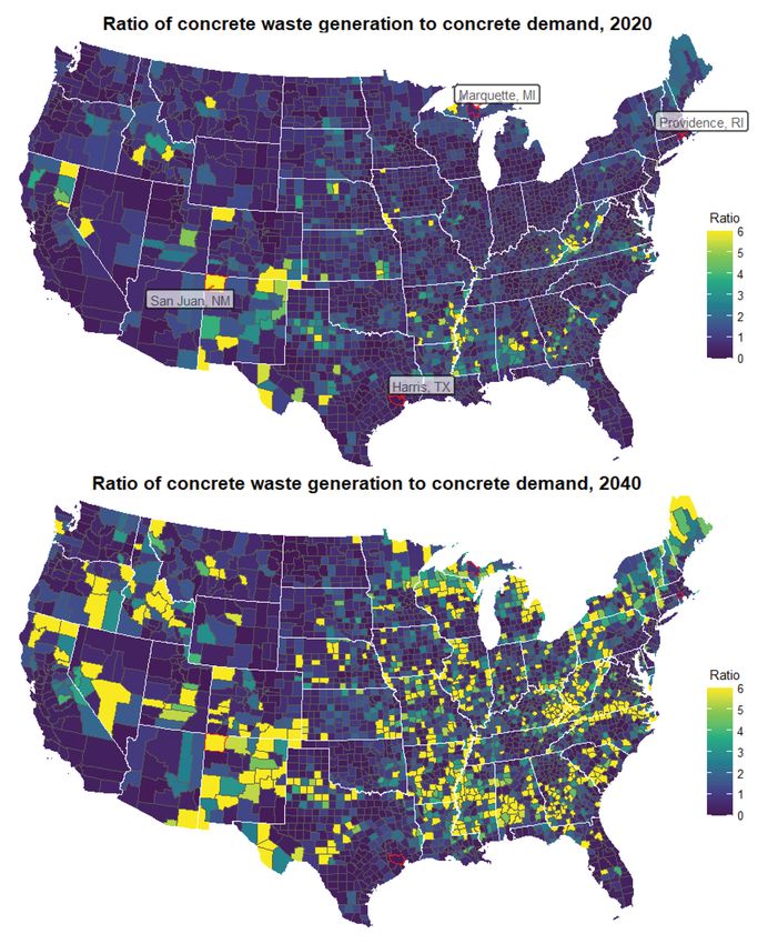
The comparison of material in- and outflows at the local level can be used to estimate potential
for material reuse within a limited geographic area. Figure 8 shows the ratio of demolition and
construction-related concrete out- and inflows for all counties in 2020 and 2040. Similar figures
for concrete and other materials for more years are shown in Figures S18–S20 in the supplemental
data online. A substantial number of (brightly colored) counties have outflows that are higher than
inflows in 2020. The prevalence of such counties grows considerably between 2020 and 2040.
The darker colored counties are generally higher population growth counties with positive stock
growth. In such locations new construction is high enough to create opportunities for material
reuse in new construction, but the reuse of waste materials will be far from sufficient to supply
the total materials requirements for new construction. In bright colored counties, a larger portion
of new construction could make use of materials sourced from demolition activities, but the
overall demand for new construction is lower, decreasing the potential for material reuse in new
construction. In the nation as a whole, the ratio of demolition to construction-related material
flows grows from 0.25–0.35 (depending on the scenario) in 2020 to about 0.45–0.55 in 2060 (see
Figure S21 in the supplemental data online). The progression of overall vacancy rates 2020–50 is
shown by county in Figure S22 in the supplemental data online.Berrill & Hertwich 611
Buildings and Cities
DOI: 10.5334/bc.126
Figure 8: Ratio of concrete
waste generation to demand
for US counties, 2020 and 2040.
5. DISCUSSION
Given the long lifetime of housing in the US (most recently estimated as 130 years on average;
Ianchenko et al. 2020), and the slowdown in stock turnover observed in some areas, due in part to
local regulations (Reyna & Chester 2015), there may be an energy-efficiency-based rationale for
increasing the rate at which new housing replaces old housing. The potential benefits of increased
stock turnover for reducing total (embodied and energy-related) residential GHG emissions are,
however, unclear. Because new houses tend to be much larger than older houses, housing stock
growth and turnover causes floor area per person to increase steadily in most scenarios (Figure 4).
This increase would be accelerated by higher turnover rates, reducing some of the energy efficiency
benefits of newer housing (Viggers et al. 2017). Further, higher turnover clearly entails higher
material flows and embodied emissions. Whether the energy and GHG reductions associated
with more efficient newer housing would outweigh the floor area increases and additional
embodied emissions is an important question which will be addressed in future research. The
high turnover scenarios would produce a greater opportunity for material reuse, as the number
of redundant vacant units (in excess of the natural vacancy rate) would be reduced (see Figure
S23 in the supplemental data online), and their materials would become available for potentialreuse. GHG benefits from material recycling or reuse are not assessed in this model, but increased Berrill & Hertwich 612
Buildings and Cities
recycling may reduce emissions from new construction. The potential for material reuse could be DOI: 10.5334/bc.126
investigated at a local level by adopting a continuous-MFA approach, accounting for the recovery
and processing losses and reuse potential for secondary materials (Schiller et al. 2017a). Emission
reductions from circular reuse of materials are not guaranteed, and depend on many factors,
including the ability to displace primary material production, local demand for reuse, and level of
material transport required (Andersen et al. 2020; Zink & Geyer 2019).
Both increasing the share of multifamily population and reducing the size of new houses would
reliably reduce emissions from new construction, and limit the growth in floor area per person,
enabling further reductions in emissions from energy consumption. In the high multifamily
scenarios, annual additions of multifamily housing become higher than additions from single-
family around 2030. This would be a substantial departure from current trends, but may be
feasible if momentum to remove restrictions (including single-family zoning, minimum lot
sizes, height and density limits, and setback and parking requirements) (Gyourko et al. 2019)
on multifamily and small single-family continues to grow. Several city and state governments
across the US are considering or moving towards the removal of single-family zoning (Bliss 2021).
In addition to removing land-use restrictions, reform of other policies which hinder multifamily
development may also help to encourage smaller typologies in new construction. Federal tax
and finance regulations currently encourage single- over multifamily development (Berrill et al.
2021), while local property taxes tend to be higher for rental housing (Goodman 2006), which is
predominantly multifamily.
In reduced floor area scenarios, the average size of new single-family homes decreases from 258
to 192 m2. Limiting the construction of very large, new single-family homes may be a different
type of challenge than removing barriers to new multifamily and small single-family. Although
many policy changes (dezoning, removal of lot size and density limits, etc.) that would permit
more multifamily would also encourage smaller single-family (Gray & Furth 2019), there are other
dynamics such as household preferences (Estiri 2014) and industry structure (Carlyle 2016) which
are part of the explanation for the growth in size of new single-family homes. More research
is needed to better understand the growth in size of new single-family homes, and identify
strategies to reduce the average size of new housing (Cohen 2021). The results shown in Figure 4
illuminate the difficulty of substantially reducing floor area per person by building smaller new
housing alone. In scenario 6 with higher shares of multifamily housing and smaller single-family
in new construction, there is a very slight reduction of floor area per person from 60.2 to 58.9 m2/
cap from 2020 to 2060. This is still far higher than the range of 30–40 m2/cap used in scenarios
aimed at limiting climate change to 1.5–2.0°C (Grubler et al. 2018; Pauliuk et al. 2021; van den
Berg et al. 2021). Building smaller homes is necessary to limit the growth of m2/cap, but by itself
may at best achieve only minor reductions. More ambitious reductions of m2/cap would require
additional strategies such as increases in household size (Ivanova & Büchs 2020) or conversion of
large single-family homes into multiple housing units (Garcia et al. 2020).
Developments in material stock and flow modeling have brought about increasing spatial
resolution, particularly in studies that combine MFAs with geographic information system (GIS)
data (Haberl et al. 2021; Yang et al. 2020). Although the spatial resolution of this housing stock
model is lower than GIS-based studies, the geographical unit of US counties is still useful for
comparing local-scale material in- and outflows and the potential for local material reuse without
the need for long-distance transportation. The introduction of dynamic vacancy rates into housing
stock models is a particularly important innovation. Incorporating vacancy rates that can change
over time is an inescapable requirement for modeling building stock evolution in regions with low
or negative population growth. This is best achieved at a subnational level in order to incorporate
locally specific vacancy rates and population growth prospects (Deilmann et al. 2009; Volk et al.
2019). As most industrialized and post-industrial nations fit the low- and slowing population
growth paradigm, and with declining fertility rates globally (Vollset et al. 2020), more explicit
consideration of vacancy in housing stock models is increasingly important. The specification of
housing stock in- and outflows with reference to locally observed and regional ‘natural’ vacancyrates here represents a novel approach to housing stock modeling, and contributes to the emerging Berrill & Hertwich 613
Buildings and Cities
incorporation of vacancy in housing stock models. DOI: 10.5334/bc.126
The limitations of the model are now highlighted to identify areas that can be improved and
extended. Although the archetype approach defines material intensities based on many different
housing characteristics, age dependencies were not considered, so each archetype is assumed to
have the same material intensity regardless of year of construction. For vacancy rates, historical
average vacancy rates by house type and Census Division were assumed to represent natural
vacancy rates. This simplifies matters and overlooks regional drivers of vacancy rates such as local
regulations, economies and housing markets, land prices, etc. (Hwang & Quigley 2006). Defining
vacancy rates, and other stock characteristics such as the prominence of multifamily and smaller
housing, with reference to local restrictions (Gyourko et al. 2019) could shed light on the role of
regulations and implications of future policy changes. The results of material in- and outflows are
just a first step in assessing the potential for material recycling and reuse. Applying the continuous-
MFA method would enable the estimation of the actual potential for material reuse and related
GHG emission reductions. Finally, the results of the housing stock model are based on one scenario
of population growth. Different national and localized population trajectories could produce quite
different results. Current population trends in the US suggest that population growth in the coming
decades may be less than the ‘mid-range’ census projection that was employed in this study.
6. CONCLUSIONS
A novel housing stock model is presented for US counties incorporating dynamic vacancy rates, with
different scenarios of housing stock turnover rates and characteristics to 2060. As the growth of the
population and housing stock slows, the ratio of demolition to construction material flows grows
from 0.25–0.35 in 2020 (depending on the scenario) to 0.45–0.55 in 2060. Reducing the average
size of new single-family housing and increasing the share of multifamily in new construction
are two strategies that can reliably reduce material requirements and embodied emissions from
housing stock growth. Both strategies would represent substantial departures from current trends,
and would require policy changes to remove existing barriers and disincentives to multifamily and
small single-family housing. Increasing stock turnover would accelerate the growth in floor area
per person and increase emissions from residential construction.
AUTHOR AFFILIATIONS
Peter Berrill 0000-0003-1614-3885
Center for Industrial Ecology, Yale University, New Haven, CT, US
Edgar G. Hertwich 0000-0002-4934-3421
Department of Energy and Process Engineering, Norwegian University of Science and Technology, Trondheim,
Norway
COMPETING INTERESTS
The authors have no competing interests to declare.
ETHICAL APPROVAL
Ethics approval was not required for this research
FUNDING
This material is based on work supported by the US Department of Energy’s Office of Energy
Efficiency and Renewable Energy (EERE) under the Advanced Manufacturing Office (award number
DE-EE0007897).This study was prepared as an account of work sponsored by an agency of the US government. Berrill & Hertwich 614
Buildings and Cities
Neither the US government nor any agency thereof, nor any of their employees, makes any DOI: 10.5334/bc.126
warranty, express or implied, or assumed any legal liability or responsibility for the accuracy,
completeness, or usefulness of any information, apparatus, product, or process disclosed, or
represents that its use would not infringe privately owned rights. Reference herein to any specific
commercial product, process, or service by trade name, trademark, manufacturer, or otherwise
does not necessarily constitute or imply its endorsement, recommendation, or favoring by the US
government or any agency thereof. The views and opinions of the authors expressed herein do not
necessarily state or reflect those of the US government or any agency thereof.
SUPPLEMENTAL DATA
Supplemental data for this article can be accessed at: https://doi.org/10.5334/bc.126.s1
Readers can also access the source data, modelling code (executed using the R software
environment), and data outputs used and produced for this research at the following public
repository: https://github.com/peterberr/US_county_HSM
REFERENCES
Andersen, C. E., Kanafani, K., Zimmermann, R. K., Rasmussen, F. N., & Birgisdóttir, H. (2020). Comparison of
GHG emissions from circular and conventional building components. Buildings and Cities, 1(1), 379–392.
DOI: https://doi.org/10.5334/bc.55
Athena Sustainable Materials Institute. (2020). Athena impact estimator v5.4. https://calculatelca.com/
software/impact-estimator/
Augiseau, V., & Barles, S. (2017). Studying construction materials flows and stock: A review. Resources,
Conservation and Recycling, 123, 153–164. DOI: https://doi.org/10.1016/j.resconrec.2016.09.002
Berrill, P., Gillingham, K. T., & Hertwich, E. G. (2021). Linking housing policy, housing typology, and
residential energy demand in the United States. Environmental Science & Technology, acs.est.0c05696.
DOI: https://doi.org/10.1021/acs.est.0c05696
Bliss, L. (2021, March 1). The upzoning wave finally catches up to California. Bloomberg City Lab. https://www.
bloomberg.com/news/articles/2021-03-01/california-turns-a-corner-on-single-family-zoning
Carlyle, E. (2016). New homes in the US are getting larger. Here’s why. Construction Dive. https://www.
constructiondive.com/news/new-homes-in-the-us-are-getting-larger-heres-why/427018/
Cohen, M. J. (2021). New conceptions of sufficient home size in high-income countries: Are we approaching a
sustainable consumption transition? Housing, Theory and Society, 38(2), 173–203. DOI: https://doi.org/10
.1080/14036096.2020.1722218
Deetman, S., Marinova, S., van der Voet, E., van Vuuren, D. P., Edelenbosch, O., & Heijungs, R. (2020).
Modelling global material stocks and flows for residential and service sector buildings towards 2050.
Journal of Cleaner Production, 245, 118658. DOI: https://doi.org/10.1016/j.jclepro.2019.118658
Deilmann, C., Effenberger, K. H., & Banse, J. (2009). Housing stock shrinkage: Vacancy and demolition
trends in Germany. Building Research & Information, 37(5–6), 660–668. DOI: https://doi.
org/10.1080/09613210903166739
Eggers, F. J., & Moumen, F. (2016). Components of inventory change: 2011–2013. https://www.huduser.gov/
portal/datasets/cinch/cinch13/cinch11-13.pdf
Eggers, F. J., & Moumen, F. (2020). American Housing Survey: Components of inventory change 2015–2017.
https://www.huduser.gov/portal/datasets/cinch/cinch15/National-Report.pdf
EIA. (2021). Monthly energy review May 2021. Monthly Energy Review. US Energy Information Administration
(EIA). https://www.eia.gov/totalenergy/data/monthly/
Ellsworth-Krebs, K. (2019). Implications of declining household sizes and expectations of home comfort for
domestic energy demand. Nature Energy, 5, 1–6. DOI: https://doi.org/10.1038/s41560-019-0512-1
Estiri, H. (2014). Building and household X-factors and energy consumption at the residential sector. A
structural equation analysis of the effects of household and building characteristics on the annual
energy consumption of US residential buildings. Energy Economics, 43, 178–184. DOI: https://doi.
org/10.1016/j.eneco.2014.02.013
Garcia, D., Tucker, J., & Schmidt, I. (2020). Single-family zoning reform: An analysis of SB 1120. https://
ternercenter.berkeley.edu/research-and-policy/single-family-zoning-reform-an-analysis-of-sb-1120/Goodman, J. (2006). Houses, apartments, and the incidence of property taxes. Housing Policy Debate, 17(1), Berrill & Hertwich 615
Buildings and Cities
1–26. DOI: https://doi.org/10.1080/10511482.2006.9521558
DOI: 10.5334/bc.126
Gray, M. N., & Furth, S. (2019). Do minimum-lot-size regulations limit housing supply in Texas? SSRN
Electronic Journal. DOI: https://doi.org/10.2139/ssrn.3381173
Grubler, A., Wilson, C., Bento, N., Boza-Kiss, B., Krey, V., McCollum, D. L., Rao, N. D., Riahi, K., Rogelj, J.,
Stercke, S., Cullen, J., Frank, S., Fricko, O., Guo, F., Gidden, M., Havlík, P., Huppmann, D., Kiesewetter,
G., Rafaj, P., … Valin, H. (2018). A low energy demand scenario for meeting the 1.5°C target and
sustainable development goals without negative emission technologies. Nature Energy, 3(6), 515. DOI:
https://doi.org/10.1038/s41560-018-0172-6
Gyourko, J., Hartley, J., & Krimmel, J. (2019). The local residential land use regulatory environment across
U.S. housing markets: Evidence from a new Wharton Index (Working Paper No. 26573). Cambridge, MA:
National Bureau of Economic Research (NBER). http://www.nber.org/papers/w26573%0ANATIONAL. DOI:
https://doi.org/10.3386/w26573
Haberl, H., Wiedenhofer, D., Schug, F., Frantz, D., Virág, D., Plutzar, C., Gruhler, K., Lederer, J., Schiller, G.,
Fishman, T., Lanau, M., Gattringer, A., Kemper, T., Liu, G., Tanikawa, H., van der Linden, S., & Hostert, P.
(2021). High-resolution maps of material stocks in buildings and infrastructures in Austria and Germany.
Environmental Science and Technology, 55(5), 3368–3379. DOI: https://doi.org/10.1021/acs.est.0c05642
Hauer, M. E. (2019). Population projections for U.S. counties by age, sex, and race controlled to shared
socioeconomic pathway. Scientific Data, 6, 1–15. DOI: https://doi.org/10.1038/sdata.2019.5
Hertwich, E. G., Lifset, R., Pauliuk, S., Heeren, N., Ali, S., Tu, Q., Ardente, F., Berrill, P., Fishman, T., Kanaoka,
K., Kulczycka, J., Makov, T., Masanet, E., & Wolfram, P. (2020). Resource efficiency and climate
change: Material efficiency strategies for a low-carbon future. Zenodo. DOI: https://doi.org/10.5281/
zenodo.3542680
Hwang, M., & Quigley, J. M. (2006). Economic fundamentals in local housing markets: Evidence from U.S.
metropolitan regions. Journal of Regional Science, 46(3), 425–453. DOI: https://doi.org/10.1111/j.1467-
9787.2006.00480.x
Ianchenko, A., Simonen, K., & Barnes, C. (2020). Residential building lifespan and community turnover.
Journal of Architectural Engineering, 26(3), 04020026. DOI: https://doi.org/10.1061/(ASCE)AE.1943-
5568.0000401
Ivanova, D., & Büchs, M. (2020). Household sharing for carbon and energy reductions: The case of EU
countries. Energies, 13(8), 1909. DOI: https://doi.org/10.3390/en13081909
Jelinski, L. W., Graedel, T. E., Laudise, R. A., McCall, D. W., & Patel, C. K. (1992). Industrial ecology: Concepts
and approaches. Proceedings of the National Academy of Sciences, USA, 89(3), 793–797. DOI: https://doi.
org/10.1073/pnas.89.3.793
Jones, C. (2019). Inventory of Carbon and Energy (ICE) V3.0. https://circularecology.com/embodied-carbon-
footprint-database.html
Krausmann, F., Wiedenhofer, D., & Haberl, H. (2020). Growing stocks of buildings, infrastructures and
machinery as key challenge for compliance with climate targets. Global Environmental Change, 61,
102034. DOI: https://doi.org/10.1016/j.gloenvcha.2020.102034
Lanau, M., Liu, G., Kral, U., Wiedenhofer, D., Keijzer, E., Yu, C., & Ehlert, C. (2019). Taking stock of built
environment stock studies: Progress and prospects. Environmental Science and Technology, 53(15),
8499–8515. DOI: https://doi.org/10.1021/acs.est.8b06652
Langevin, J., Reyna, J. L., Ebrahimigharehbaghi, S., Sandberg, N., Fennell, P., Nägeli, C., Laverge, J.,
Delghust, M., Mata, Van Hove, M., Webster, J., Federico, F., Jakob, M., & Camarasa, C. (2020).
Developing a common approach for classifying building stock energy models. Renewable and
Sustainable Energy Reviews, 133(December 2019). DOI: https://doi.org/10.1016/j.rser.2020.110276
McCue, D. (2018). Updated household growth projections: 2018–2028 and 2028–2038. https://www.jchs.
harvard.edu/sites/default/files/Harvard_JCHS_McCue_Household_Projections_Rev010319.pdf
Müller, D. B. (2006). Stock dynamics for forecasting material flows—Case study for housing in The
Netherlands. Ecological Economics, 59(1), 142–156. DOI: https://doi.org/10.1016/j.ecolecon.2005.09.025
NREL. (2020). ResStock housing characteristics (ResStock v2.3.0). https://github.com/NREL/OpenStudio-
BuildStock/tree/master/project_national/housing_characteristics
O’Neill, B. C., Kriegler, E., Ebi, K. L., Kemp-Benedict, E., Riahi, K., Rothman, D. S., van Ruijven, B. J., van
Vuuren, D. P., Birkmann, J., Kok, K., Levy, M., & Solecki, W. (2017). The roads ahead: Narratives for
shared socioeconomic pathways describing world futures in the 21st century. Global Environmental
Change, 42, 169–180. DOI: https://doi.org/10.1016/j.gloenvcha.2015.01.004
Pauliuk, S., & Heeren, N. (2020). Material efficiency and its contribution to climate change mitigation in
Germany: A deep decarbonization scenario analysis until 2060. Journal of Industrial Ecology, 25(2),
479–493. DOI: https://doi.org/10.1111/jiec.13091You can also read