Large scale variations in the dynamics of Amazon forest canopy gaps from airborne lidar data and opportunities for tree mortality estimates
←
→
Page content transcription
If your browser does not render page correctly, please read the page content below
www.nature.com/scientificreports
OPEN Large‑scale variations
in the dynamics of Amazon forest
canopy gaps from airborne lidar
data and opportunities for tree
mortality estimates
Ricardo Dalagnol1*, Fabien H. Wagner1,2, Lênio S. Galvão1, Annia S. Streher1,
Oliver L. Phillips3, Emanuel Gloor3, Thomas A. M. Pugh4,5, Jean P. H. B. Ometto6 &
Luiz E. O. C. Aragão1,7
We report large-scale estimates of Amazonian gap dynamics using a novel approach with large
datasets of airborne light detection and ranging (lidar), including five multi-temporal and 610 single-
date lidar datasets. Specifically, we (1) compared the fixed height and relative height methods for gap
delineation and established a relationship between static and dynamic gaps (newly created gaps); (2)
explored potential environmental/climate drivers explaining gap occurrence using generalized linear
models; and (3) cross-related our findings to mortality estimates from 181 field plots. Our findings
suggest that static gaps are significantly correlated to dynamic gaps and can inform about structural
changes in the forest canopy. Moreover, the relative height outperformed the fixed height method
for gap delineation. Well-defined and consistent spatial patterns of dynamic gaps were found over
the Amazon, while also revealing the dynamics of areas never sampled in the field. The predominant
pattern indicates 20–35% higher gap dynamics at the west and southeast than at the central-east and
north. These estimates were notably consistent with field mortality patterns, but they showed 60%
lower magnitude likely due to the predominant detection of the broken/uprooted mode of death.
While topographic predictors did not explain gap occurrence, the water deficit, soil fertility, forest
flooding and degradation were key drivers of gap variability at the regional scale. These findings
highlight the importance of lidar in providing opportunities for large-scale gap dynamics and tree
mortality monitoring over the Amazon.
There is increasing evidence showing that tree mortality is a key factor for understanding carbon storage and
sequestration in the Amazon f orests1, 2. Specifically, the majority of the mortality events are related to very fre-
quent small- to intermediate- scale disturbances (< 5 ha) rather than episodic large-scale events (> 5 ha)3. How-
ever, the uncertainties associated with tree mortality drivers and mechanisms, especially at smaller scales (< 1 ha),
constrain our ability to accurately measure tropical forest carbon budget and assess climate change e ffects4.
Tree mortality in the Amazon has been apparently increasing since the past decade likely due to greater
climate variability and feedbacks of faster growth and mortality. This has effectively shortened tree life cycles5.
Overall, tree mortality drivers acting from regional to local scales may include water stress or d rought6, soil
fertility7, wind disturbances8, 9, flooding10, 11, lightning12, 13, liana abundance and s hading2. Human-related fac-
tors also affect mortality rates, such as forest degradation, fragmentation and edge e ffects14, 15. These drivers can
1
Earth Observation and Geoinformatics Division, National Institute for Space Research-INPE, São José dos
Campos, SP 12227‑010, Brazil. 2GeoProcessing Division, Foundation for Science, Technology and Space
Applications-FUNCATE, São José dos Campos, SP 12210‑131, Brazil. 3School of Geography, University of
Leeds, Leeds LS2 9JT, UK. 4School of Geography, Earth and Environmental Sciences, University of Birmingham,
Birmingham B15 2TT, UK. 5Birmingham Institute of Forest Research, University of Birmingham, Birmingham B15
2TT, UK. 6Earth System Sciences Center, National Institute for Space Research-INPE, São José dos Campos,
SP 12227‑010, Brazil. 7Geography, College of Life and Environmental Sciences, University of Exeter, Exeter EX4
4RJ, UK. *email: ricds@hotmail.com
Scientific Reports | (2021) 11:1388 | https://doi.org/10.1038/s41598-020-80809-w 1
Vol.:(0123456789)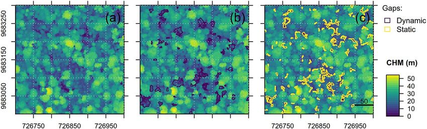
www.nature.com/scientificreports/
kill the trees through the physiological mechanisms of carbon starvation and hydraulic failure, the interactions
with biotic agents, and the modifications in plant structure that provoke stem breakage2. All this knowledge has
been originated from field observations over a few hundred-forest sites in the Amazon, but we still lack tools
for monitoring tree mortality over a large scale. To reduce the uncertainties of the mechanisms and accurately
predict environmental and climate effects over tropical forests, remote sensing is an alternative for large-scale
assessment of tree m ortality2, 16. Nevertheless, the development of remote sensing methods for this purpose is
still challenging, especially over the diverse and heterogeneous forests of the Amazon.
In principle, multi-temporal data from very high-resolution (VHR) satellites allow the estimation of tree
mortality rates over tropical forests17. However, semi-automatic retrievals of tree mortality using VHR data are
still challenging due to view-illumination effects. These effects alter the relative amounts of shadows and gaps
viewed by the VHR sensors, which generally capture only the mortality of the tallest trees18, 19. In comparison
with the VHR imagery, the multi-temporal data acquired by small-footprint airborne lidar instruments allow
a more precise estimation of canopy gaps that can be related to tree loss at the canopy level19–21. On the other
hand, standing dead trees do not necessarily generate gaps18 and airborne lidar mainly observes the upper-canopy
trees in detail. As a result, the estimates of mortality from lidar canopy gaps are likely biased to some extent on
observing tree mortality associated with broken and uprooted mode of death. In the Amazon, this mode of death
represents approximately 39–55% of the total mortality but, on average, it is not significantly distinguished from
the standing dead mode of d eath22–24.
The traditional gap concept consists of a ‘hole’ in the forest canopy extending through all levels down to an
average height of 2 m above the ground25. A gap is created by the treefall of one or more trees, from either natu-
ral mortality or human-induced disturbances. There are two types of gaps reported in the l iterature21: (1) static
gaps observed in a single-date lidar acquisition, showing the aggregated effects of gap opening and vegetation
regeneration over time; and (2) dynamic gaps observed using two repeated lidar acquisitions, representing newly
opened gaps from one date to another. However, the measurement of gaps is still challenging even using lidar.
For instance, different gap definitions based on height cutoffs have provided different measurements of static
gaps21, 26, 27. Alternatively, the height cutoff can be calibrated to a forest site based on the statistical analysis of the
canopy height distribution10. However, this approach does not account for factors such as the presence of large
open areas that are not necessarily treefall gaps. In temperate forests, another gap definition has been adopted
considering the canopy relative height (RH) in relation to its n eighborhood28. Nevertheless, this approach has
not yet been tested over tropical forests.
The drivers of small-scale gap dynamics are also not completely understood. Local studies over Neotropi-
cal forests have shown that the topography, proxied by the Height Above the Nearest Drainage (HAND) index
and terrain slope, can affect the gap dynamics with mechanisms related to wind exposure and waterlogged
areas10, 22, 23, 29. Some forests showed gaps more frequently at valleys that increased in size toward the high ter-
rain slopes10, 23, 29. Other forests did not show such relationships22. A study on small-scale gaps using Landsat
satellite data have also pointed out for the effect of wind on opening gaps between 80 and 1000 m230. Storms and
lightning were also reported as the main causes of mortality in a forest at central A mazon12. Nevertheless, even
considering these studies, not much is known regarding the variability of small-scale gaps along environmental
and climate gradients across the Amazon region.
In this context, the analysis of lidar gap dynamics can significantly improve our comprehension on gap
dynamics and tree mortality at a large scale in the Amazon. This is especially true given the new opportunities of
increased lidar spatial coverage across the Brazilian Amazon. In 2016, 610 non-overlapping airborne lidar flight
lines (300 m × 12.5 km) were obtained by the Improving Biomass Estimation Methods for the Amazon (EBA)
project of the Brazilian National Institute for Space Research (INPE)31. Along with a few available multi-temporal
lidar flight lines, such unique datasets can be used to evaluate drivers of gap dynamics and assess opportuni-
ties for correlations with field-measured tree mortality. The analysis of these datasets can bring new insights of
forest dynamics patterns, drivers and mechanisms, and even guide the planning of new fieldwork activities for
measuring tree mortality in the Amazon.
Here, we present the first large-scale study of lidar gap dynamics in the Amazon. The main goal was to provide
a systematic assessment of canopy gaps across environmental-climate gradients and evaluate the possibilities
of tree mortality estimates over tropical forests. Specifically, we aimed to answer the following research ques-
tions: (Q1) How are static and dynamic canopy gaps related in tropical forests and which gap definition best
represents this relationship? (Q2) How do canopy gap dynamics derived from airborne lidar data vary across
the Brazilian Amazon forests? (Q3) What landscape- and/or regional-scale factors drive gap variability in the
Brazilian Amazon? (Q4) Does large-scale dynamic gaps estimates reproduce known spatial patterns of field-plot
tree mortality estimates across the Amazon?
To answer Q1, we assessed the relationship between static and dynamic gaps using five multi-temporal
airborne lidar datasets acquired over five test sites in Brazil with distinct forest types, vegetation structure and
biomass. To answer Q2 and Q3, we evaluated the spatial variability of canopy gaps and some of the main drivers
across the Brazilian Amazon. We used single-date airborne lidar data acquired in 610 non-overlapping lidar
flight lines, representing a total sampled area of ~ 2300 km2. To answer Q4, we combined outputs from the previ-
ous analyses to estimate Amazon-wide dynamic gaps and related these estimates with tree mortality rates from
long-term field inventory data.
Results
Multi‑temporal lidar analysis of static and dynamic gaps relationship. The spatial matching
between static and dynamic gaps showed variable responses amongst different combinations of methods and
parameters explored on the five test sites (Sites-average F1-Score (F) from 0.01 to 0.51; detailed results in Sup-
Scientific Reports | (2021) 11:1388 | https://doi.org/10.1038/s41598-020-80809-w 2
Vol:.(1234567890)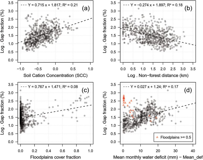
www.nature.com/scientificreports/
Figure 1. Example of the spatial match between canopy tree mortality (black) and gap delineation (yellow)
based on relative height (RH = 50, W = 5) at the TAP site. The background is a Canopy Height Model (CHM) for
the year 2012 in (a), and the year 2017 in (b) and (c). R v4.0.2 was used to plot this figure32.
Figure 2. Relationship between static gap fraction (%) and annualized dynamic gap fraction (% y ear−1) for 5-ha
plot areas (n = 780) over the five studied sites (DUC, TAP, FN1, BON, and TAL).
plementary Table S1). The RH delineation method, considering 50% maximum height on a 5-m window (W)
neighborhood (RH = 50, W = 5), showed the best overall result (Sites-average: F = 0.51, precision (p) = 0.42, recall
(r) = 0.66). When excluding the gaps pre-existing in the first lidar acquisition, an upper-bound performance esti-
mate for this method indicated a modest increase in p and F (Sites-average: F = 0.62, p = 0.61, r = 0.66). The best
result amongst the sites for the fixed height method was based on a 10-m height cutoff (Sites-average: F = 0.48,
p = 0.47, r = 0.55), showing an inferior performance than the RH method.
The correspondence between static and dynamic gaps for the best method (RH = 50, W = 5) is illustrated in
Fig. 1A–C. The dynamic gaps detected between 2012 and 2017 are shown in black (Fig. 1B) and the static gaps
from 2017 data are represented in yellow (Fig. 1C) for a small subset of the TAP site. The method was able to map
68% of the dynamic gap areas ( rTAP = 0.68), with commission errors ranging from 34% ( pTAP = 0.66, upper-bound
estimate) to 58% (pTAP = 0.42, lower-bound estimate; Supplementary Table S1). For instance, in Fig. 1C, the top-
right area showed examples of commission errors, i.e. delineated static gaps that do not correspond to dynamic
gaps. Meanwhile, the bottom-middle area showed static gaps that successfully matched the dynamic gaps.
In a detailed inspection of the forest vertical structure prior to gap creation, we observed that static gaps
detected dynamic gaps associated with trees below (< − 5 m, 98.5% accuracy) or close to the mean local canopy
height (between − 5 and 5 m, 77% accuracy) with greater accuracy than that observed for trees above it (> 5 m,
37% accuracy) (Supplementary Figure S1). Correct detections below and close to the mean local canopy height
represented 80.6% of the total dynamic gaps (15,582 out of 19,324 events).
When we aggregated the gap detections to gap fraction at larger scales (5 ha plot area), we observed a sig-
nificant, positive and non-linear logarithmic relationship between static gap fraction and annualized dynamic
Scientific Reports | (2021) 11:1388 | https://doi.org/10.1038/s41598-020-80809-w 3
Vol.:(0123456789)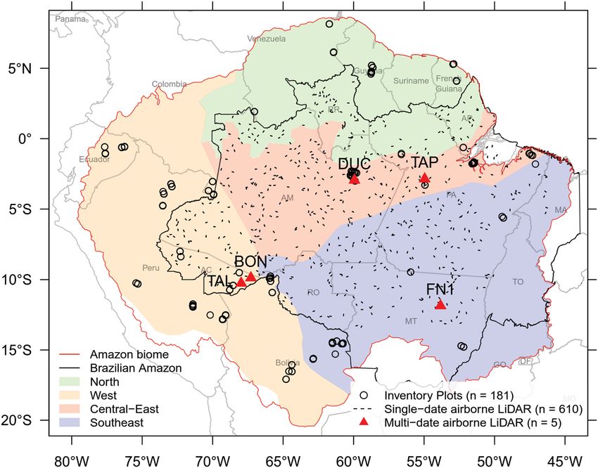
www.nature.com/scientificreports/
Figure 3. Canopy gaps based on the relative height (RH = 50, W = 5) across the Brazilian Amazon (n = 610 flight
lines). (a) Gap fraction (%). (b) Mean gap size (m2).
gap fraction (R2 = 0.705 ± 0.08, RMSE = 38.3 ± 13%; Fig. 2). The model residuals were randomly distributed.
The uncertainty on estimating dynamic gap fraction from static gaps increased from small to higher static
gap fraction values, as highlighted by the increasing prediction interval band. The sites with the highest mean
static gap fraction estimates (mean ± SD%, n = number of samples), in decreasing order, corresponded to TAL
(11.18 ± 3.97%, n = 69), BON (8.07 ± 4.28%, n = 95), TAP (6.4 ± 2.25%, n = 183), FN1 (3.3 ± 2.06%, n = 199), and
DUC (1.47 ± 0.60%, n = 234).
Single‑date lidar gap spatial variability and drivers across the Brazilian amazon. Spatial vari-
ability of static gaps. The Brazilian Amazon region showed static gap fraction values ranging from 0.7 to 22.3%
(Fig. 3A). The average gap fraction was 4.11%, but the majority of gap fraction values were lower than 5.17%
(75th percentile). An overall lower gap fraction (Fig. 3A) was observed at central-east (mean ± SD: 3.57% ± 3.05)
and north (3.68% ± 2) of the Amazon than at west (4.18% ± 2.13) and southeast (4.89% ± 2.47) regions of the
study area described in Methods. High gap fraction values (> 5.17%) were found over the Brazilian states of
Pará (~ 52° W; 5° S) and Acre (~ 69° W; 10° S). They were observed close to major water streams, such as the
Amazonas and Madeira rivers, and to floodplains near the center of the Amazonas state (~ 65° W; 4° S). Besides
these locations nearby rivers, predominantly lower gap fractions (< 2%) were found at the northwest Brazilian
region over the Amazonas state. In comparison to other regions, the northwest has more intact forests, less water
deficit and is expected to have increased AGB stocks. One site with anomalous high gap fraction (22.3%) was
observed in eastern Amazon over the Arariboia indigenous land (~ 46° W; 5° S). This area has been degraded in
recent years through illegal logging and fire. The gap fraction at the southeastern Xingu forests (~ 53° W; 12° S)
ranged from 1.9 to 7.5%, with an average of 4.3%. This range of variability is likely lower than expected for one of
the regions with most negative water deficit. The spatial variability of gap fraction (Fig. 3A) was consistent with
the canopy height variability (Supplementary Figure S2). For instance, areas with high gap fraction showed the
largest variation in canopy heights ( CHMSD from 8 to 14 m) and the lowest “minimum” height ( CHMP05 < 10 m).
The mean gap size (Fig. 3B) followed a similar spatial pattern as the gap fraction (Fig. 3A), with an average gap
size across sites of 40.89 m2. Only a few sites showed larger mean gap sizes (> 100 m2).
Landscape‑ and regional‑scale drivers of static canopy gaps. At the landscape-scale level, that is, within each
lidar flight line, the HAND and slope variables were not able to explain gap occurrence or gap size ( m2) vari-
ability (R2 ≈ 0). The same lack of relationship was observed by including/excluding the site as a random factor
in the generalized linear models (GLM).
At the regional-scale level, that is, analyzing aggregated static gap fraction across sites, all tested variables
were significantly correlated to gap fraction (p < 0.01) with absolute Pearson’s r values ranging from 0.21 to 0.46
(Supplementary Table S2). Seven variables were selected for modeling given their stronger correlation with gap
fraction and lower correlation amongst themselves (r < 0.7): soil fertility proxied by Soil Cation Concentration
(SCC); forest degradation proxied by non-forest distance (Nonforest_dist); Floodplains cover; water deficit proxied
by Mean_def and SD_def; and wind speed proxied by Mean_vs and SD_vs.
Three GLMs were empirically tested to estimate static gap fraction (Table 1, Supplementary Table S3): a
full model with all seven variables (R2 = 0.557, RMSE = 52 ± 10%); a simplified model excluding wind variables
and SD_def which were the least contributing variables (R2 = 0.523, RMSE = 53.3 ± 9.8%); and a final model
based on the simplified model but including an interaction term between Mean_def and Floodplains (R2 = 0.57,
RMSE = 44.9 ± 6%). All models showed randomly distributed residuals versus fitted values and were significantly
different from a null model (p < 0.001). The final model achieved a superior gap fraction explanation than the
full model and lower error, although not statistically different from each other (p = 1). Nevertheless, the final
model showed a lower BIC value, indicating a better fit with more parsimony amongst the predictors and a lower
multicollinearity (all VIF < 2). The final model residuals showed weak but significant spatial correlation effects
Scientific Reports | (2021) 11:1388 | https://doi.org/10.1038/s41598-020-80809-w 4
Vol:.(1234567890)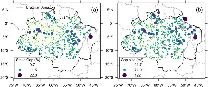
www.nature.com/scientificreports/
Model variables ΔR2 B SE B β t P value VIF
(Intercept) – 1.65 0.05 – 30.6 < 0.01 -
SCC 0.16 0.69 0.05 0.20 15.25 < 0.01 1.17
Nonforest_dist 0.03 − 0.13 0.02 − 0.09 − 6.3 < 0.01 1.39
Floodplains 0.17 1.63 0.10 0.08 15.75 < 0.01 1.94
Mean_def 0.09 0.03 0.002 0.12 11.15 < 0.01 1.68
Floodplains:Mean_def 0.05 − 0.11 0.01 − 0.12 − 8.39 < 0.01 1.61
Table 1. Estimated regression parameters (B), standard errors (SE B), t values (t) and p values for the
generalized linear model (GLM) to estimate gap fraction. Standardized beta coefficients (β), ΔR2 (change in
R2 by adding the variable last to the model) and variance-inflation factors (VIF) for each predictor were also
reported. Model achieved R2 of 0.57. SCC soil cation concentration, Nonforest_dist distance to the nearest non-
forest area, Floodplains floodplains cover fraction, Mean_def mean monthly water deficit.
Figure 4. Relationships between gap fraction (log-scale) and predictors used in the final model. (a) Soil
cation concentration (SCC). (b) Non-forest distance (km) (log-scale). (c) Floodplains cover fraction. (d) Mean
monthly water deficit (mm)—Mean_def. Red triangles on panel (d) represent samples with floodplains cover
fraction ≥ 0.5. The dashed line represents a linear model.
(Moran’s I = 0.27, p < 0.01). However, the model parameter estimates and interpretations were not different from
those from a model accounting for the spatial correlation (Supplementary Table S4).
All predictors in the final model showed significant effects on gap fraction (p < 0.01) (Table 1). The predic-
tors SCC, Floodplains, and Mean_def presented positive regression coefficients (B), indicating that an increase
in these predictors caused an increase in gap fraction. In contrast, the Nonforest_dist and Floodplains:Mean_def
had a negative B. These coefficient signs were corroborated by the expected relationship between these predictors
and gap fraction (Fig. 4A–D). Floodplains and SCC solely explained the most gap fraction variability (ΔR2 = 0.17
and 0.16, respectively). The order of predictors’ importance ranked from the largest to the smallest absolute β
values corresponding to: SCC, Mean_def, Floodplains:Mean_def, Nonforest_dist, and Floodplains. The Floodplains
variable showed the lowest β, but part of its explained variability was also shared with the interaction term, thus
Scientific Reports | (2021) 11:1388 | https://doi.org/10.1038/s41598-020-80809-w 5
Vol.:(0123456789)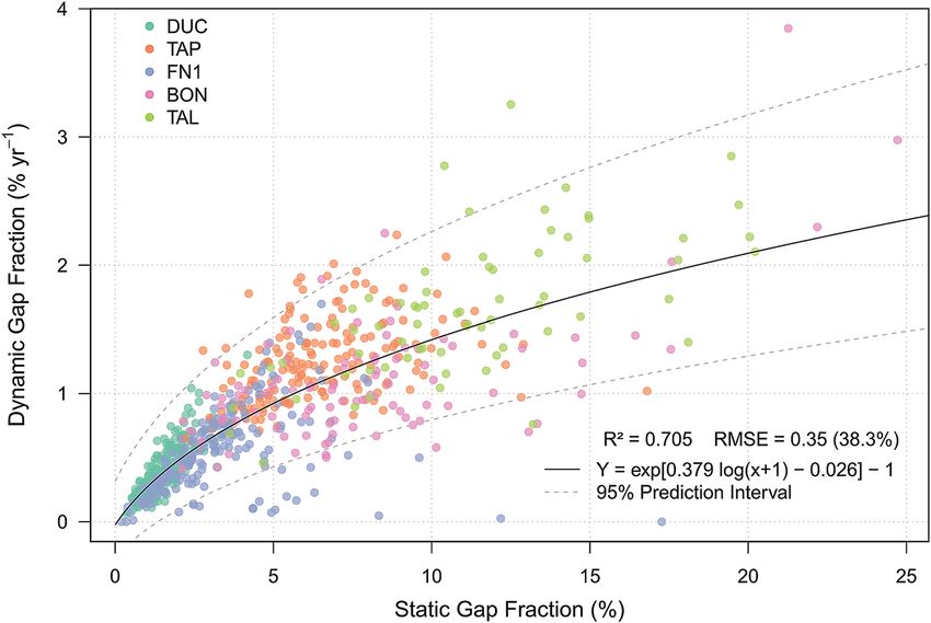
www.nature.com/scientificreports/
Figure 5. Large-scale estimates of dynamic gaps and relationship with tree mortality. (a) Dynamic gap (%
y ear−1) generated at 5-km spatial resolution from the lidar static-dynamic gaps relationship (Fig. 3) and gap/
environmental-climate model (Table 1). (b) Relationship between estimated dynamic gap fraction and field-
based tree mortality from Brienen et al.5. (c) Estimated dynamic gap (% y ear−1) per Amazonian region using
all values from the map (in blue, n > 40,000 pixels per boxplot) and just those corresponding to the field-plot
locations (in orange, n = 88). The mean dynamic gap was statistically different between regions (p < 0.01).
Dashed line represents the 1:1 line. R v4.0.2 was used to plot this figure32.
it had more effect on gap fraction than Nonforest_dist. The interaction term (Floodplains:Mean_def) caused a
significant improvement over the simplified model (Supplementary Table S3), likely associated with a better
representation of areas with high gap fraction and close to zero water deficit areas, i.e. flooded or seasonally-
flooded forests (red triangles in Fig. 4D).
Amazon‑wide dynamic gaps map and opportunities for tree mortality estimates. The dynamic gap fraction map
showed diverse forest dynamics across the Amazon (Fig. 5A). Overall, lower dynamic gap fractions (< 0.5%
year−1) were found at the undisturbed and wetter regions of the central-east, north and west Amazon. In contrast,
higher dynamic gap fractions (> 1.5% year−1) were notably found over seasonally flooded forests, such as in the
bottom-left of southeast Amazon (e.g. Noel Kempff Mercado National Park), west Amazon (e.g. Pacaya-Samiria
Scientific Reports | (2021) 11:1388 | https://doi.org/10.1038/s41598-020-80809-w 6
Vol:.(1234567890)www.nature.com/scientificreports/
National Reserve) and central-east Amazon (e.g. along Amazonas and Madeira rivers). Forests bordering the
Andes at the southwest or in the transition zone with the Brazilian savannas (Cerrado) at the east also showed
high dynamic gap fraction. These areas in the east have also a very high mean monthly water deficit (> 40 mm)
(Supplementary Figure S4B). The spatialized SD of gap fraction estimates (Supplementary Figure S3B) indicated
larger uncertainty over the southeast and west areas with higher dynamic gap fraction.
The dynamic gap fraction estimates were significantly associated with field-based stem tree mortality rates
(R2 = 0.40, RMSE = 31.8% ± 9.2, Fig. 5B). However, it systematically underestimated the field mortality rates, as
lidar dynamic gap fraction estimates were on average 58% lower than plot-based mortality rates. The results
showed overall 20–35% higher annual dynamic gap fraction over the southeast (mean ± SD: 0.89% y ear−1 ± 0.2)
and west (0.8% y ear−1 ± 0.28) regions than at the central-east (0.66% y ear−1 ± 0.28) and north (0.65% y ear−1 ± 0.17)
regions (Fig. 5C). Considering all pixels over the Amazon in the analysis, we observed significant statistical dif-
ferences in mean estimated dynamic gap fraction between the regions (ANOVA test; p < 0.01). This difference was
more pronounced over the southeast Amazon, as deduced from the comparison of estimates using all pixels or
just those pixels over the plot locations (blue and orange boxplots, respectively, in Fig. 5C). Most plots over the
southeast region are located in forest fragments with fast dynamics, that is, in areas having potential high tree
mortality and recruiting. When we considered only the field plot locations, the dynamic gap differences were
also significant between regions (p < 0.01), except between central-east and north (p = 0.8).
Discussion
We provided the first large-scale assessment of gap dynamics and its environmental-climate drivers across the
Amazon forests. We also showed the opportunities for tree mortality estimates and monitoring based on the
lidar gap dynamics. The dynamic gap fraction estimates notably matched the overall spatial patterns of stem tree
mortality rates observed in the field plots, that is, the less-dynamic north and central-east regions in contrast to
the more-dynamic west and southeast r egions1, 7, 24, 33, 34. Additionally, our map indicated new findings of slower
forest dynamics observed over large regions of undisturbed forests at the northwest (Amazonas state; 53° W;
12° S) and southeast Amazon (Xingu forests at the Mato Grosso state; 53° W; 12° S), as well as faster dynamics
at eastern Amazon (near the center of Pará state; 54° W; 6° S). It also indicated high dynamic gaps for areas of
bamboo-dominated forests at the southwest Amazon (70° W; 10° S), which had higher mortality rates than the
average western forests35.
Part of this success was due to the use of the largest airborne lidar dataset already available over the Amazon
(n = 610 flight lines). This unprecedented mission brought unique data over remote areas of the Amazon forest,
where plot data collection was inexistent. Our dynamic gap estimates were about 60% lower in overall magnitude
than the field-measured stem mortality rates. In addition to the uncertainties in the data analysis, the most prob-
able explanation for the underestimation of tree mortality is the predominant detection of broken and uprooted
mode of death associated with felled trees and the opening of gaps, which are ~ 50% of the total mortality22–24.
Some standing dead trees also eventually break and fall, generating detectable gaps, but that rate is relatively low
(4% year−1)24. Furthermore, the inevitable mismatch in scale between lidar and field inventory data certainly
contributed to the observed differences in the magnitude of the estimates. The overall correlation could be partly
associated to the gradient of forests dynamics across the regions, as forests in the west and southeast are known
to have faster dynamics with increased tree mortality and productivity than the central-east and north r egions1.
Even though, their relationship was significant and relatively strong ( R2 = 0.40) for a biological process observed at
large scale, while only considering the spatial distribution of samples and not the temporal scale, and containing
uncertainties in both measurements. The dynamic gaps (per unit area per unit time) are also likely correlated to
AGB loss rate due to the predominant detection of upper-canopy trees loss. This relationship should be explored
in further studies matching geo-located field plots with airborne lidar data.
We described a novel and significant relationship between static and dynamic gaps. We showed and quanti-
fied how static gaps information derived from single-date lidar could be used to estimate dynamic gaps, that is,
structural changes in the forest canopy likely related to broken and uprooted trees. Hence, this finding opens
venues for applications of gap metrics for forest monitoring beyond the simple representation of open spaces
within the forest canopy. The developed method maps the gaps based on the relative height of 50% maximum
height on a 5-m neighborhood, and explained 70% of annual dynamic gap fraction on the five tested sites. A
potential explanation for the non-linearity on the static-dynamic gaps relationship is the gradient of canopy
structure from more closed-canopy and/or undisturbed forests to more open-canopy and/or disturbed forests.
In very dense forests, such as those from the DUC site, a static gap is highly correlated to newly created gaps from
broken/uprooted mortality. This association is less strong for open forests, such as those observed at TAL, where
gaps do not only represent mortality events but are also a part of the natural forest canopy structure. Hence, in
order to offset this canopy structural gradient from closed to open and represent higher dynamic gap fractions
(likely higher canopy turnover and mortality), an even higher static gap fraction is required.
When compared to the 10-m fixed height cutoff approach, the relative height method showed a similar but
slightly stronger relationship with dynamic gap fraction and provided a dynamic adjustment to local canopy
variability. This is very important given the high heterogeneity of the Amazon forest canopies. This results in a
more stable and trustworthy gap delineation for large-scale applications in forests of varied canopy structure.
In addition, the use of other fixed height cutoffs with lower values (2 and 5 m), traditionally adopted in tropical
forests studies21, 25, 29, did not provide significant relationships between static and dynamic gaps. This means that
the gaps detected using these thresholds are not directly related to recent canopy turnover events. Nevertheless,
we expect that this finding contribute to the debate of gap delineation, where the relative height method should
be an improvement over the fixed height cutoff approach. This is especially important if the intent is to represent
Scientific Reports | (2021) 11:1388 | https://doi.org/10.1038/s41598-020-80809-w 7
Vol.:(0123456789)www.nature.com/scientificreports/
recent structural changes in forests with varied canopy structure such as branch losses or tree losses associated
to tree mortality or human disturbances.
Even considering the limitations to represent each natural and anthropogenic factor driving gap dynamics,
our analysis detected water stress, soil fertility, floodplains and forest disturbance as key factors for predicting
gap fraction at large scales. They explained up to 57% of its variability. The gap fraction followed a similar pattern
to that of water stress in the Amazon (Supplementary Figure S4A,B), showing a gradient from the northwest
(wetter) to the southeast (drier). The water stress had been previously associated with tree mortality measured
in field plots and specifically to drought-related m ortality6, 36.
river2, probably due to the lack of soil data
Soil fertility is less often reported in the literature as a mortality d
and/or perhaps because there are not many plots in regions with large soil nutrient gradients as depicted in the
SCC product (Supplementary Figure S4C). In contrast, the lidar data here analyzed covered gradients from very
low to high nutrient concentration. In the literature, higher soil fertility in younger alluvial soils of the western
Amazon has been associated with faster forest dynamics, which, in turn, translates into higher tree m ortality7.
In our study, a few identified caveats about the SCC and its relationship with gap fraction include: (1) the rep-
resentation of just a portion of soil fertility (Ca+Mg+K); (2) uncertainties related to the interpolation method;
and (3) the soil sampling used to build the product, which was rather scarce in eastern A mazon37. These caveats
should not be ignored because the high SCC in the eastern region was coincident with part of the highest gap
fraction observations.
The observed patterns of floodplains and forest degradation (proxied by non-forest distance) (Supplemen-
tary Figure S4D) agreed with those of gap fraction. These results corroborate the literature on expected effects
of increased gaps over water-logged lowlands10, 11 and tree mortality over flooded f orests38. They corroborated
also the increased mortality with degraded and/or fragmented forests14, 15. Further studies should assess with
greater detail the gap variability with fragment edge effects, i.e. whether gap distribution significantly varies with
distance from the fragment borders.
Our analysis did not detect the effects of wind on gap dynamics at the regional scale. However, wind has
a well-known role in tropical forest mortality by uprooting trees, especially over the northwest Amazon8, 9.
Moreover, its enhanced effect on snapping and uprooting trees that went through recent fire degradation has
been demonstrated39. Our analysis does not show this effect probably because, at a regional scale, forests are
likely adapted to the average wind variability. As a result, the mean gap fraction would not be driven by the
mean wind speed. In addition, we show a much lower mean gap size (40.89 m 2) than found in a study exploring
2 30
wind mortality (360 m ) . However, as reported in previous studies, extreme wind events could produce large
forest disturbances, affecting areas even greater than 100 ha per event. Such large events are relatively rare23.
Moreover, we did not find relationships of gap occurrence and size with slope and HAND topographic variables.
The influence of topography on small-scale gaps over the relatively flat terrains of the Amazon is certainly less
pronounced than that observed in other sloped forested areas of the world.
The influence of human-induced disturbances was likely underestimated in our analysis. The proximity of
forests with high gap fractions to the ‘deforestation arch’ (agricultural frontier between savannas and tropical
forests) confirmed some degree of human disturbance on results (e.g., logging, fire, fragmentation, edge effects).
Because a reliable forest degradation product for the Amazon does not yet exist, we have attempted to assess this
effect using the distance of each pixel to the nearest non-forest area (i.e. pastures, croplands, cities, roads, rivers).
Although having a significant and negative relationship with gap fraction (i.e. the farther inside the forest, the
less gaps), the non-forest distance metric did not explain much new of gap fraction variability when compared to
other natural predictors. These disturbance effects probably consist of long-term processes (e.g., recovery from
logging or fragmentation) rather than recent episodic events15. Fire disturbance was also not directly considered
in our analysis of tree mortality. For instance, the TAL and BON sites were partially disturbed by fire before
lidar data acquisition. However, the comparison of dynamic gaps in burned and non-burned areas mapped b y40
within these sites did not show statistically significant differences between them (Supplementary Figure S5).
Fire is widely known to affect tree mortality41. However, the effect of understory fires on tree mortality depends
on fire frequency and severity.
Forest seasonality is another potential factor affecting gap fraction estimates from lidar data. In our study, the
single-date lidar data were acquired almost regularly across the year, except for March. The acquisition covered
both the rainy and dry seasons of the Amazon in 2016 (Supplementary Figure S6A). However, we did not find
evidences of a seasonality control on gap fraction, that is, larger gap fractions were not more frequently observed
in the dry season when compared to the rainy season (Supplementary Figure S6B). This was very likely related to
the filtering of gaps based on size (minimum area of 10 m2) prior to gap fraction calculation, which eliminated
potential small holes within crowns caused by leaf loss.
Our study points out for the importance of high-resolution lidar data to understand the relationships between
gap dynamics and tree mortality. The acquisition of additional multi-temporal datasets as well as field data at
poorly sampled regions in the Amazon are necessary. This would be extremely valuable to confirm patterns here
observed and to reduce uncertainties in the analysis. Future directions of investigation include: (1) the use of
additional multi-temporal lidar data (ideally annual) to confirm the magnitude of the relationships between static
and dynamic gaps as well as between dynamic gaps and canopy mortality. Such relationships should consider the
spatial and temporal scales, which may also vary across forest types and secondary successions; (2) the further
investigation of drivers that might explain the remaining gap fraction variability, including effects of lightning,
shading, and lianas2, 12, 13; (3) the exploration of orbital lidar data from the NASA’s GEDI (Global Ecosystem
Dynamics Investigation) mission. While its footprint is too large to directly observe gaps, multiple overpasses
of GEDI over the same location may capture variations in forest height associated with newly opened gaps;
and (4) the development of new methods for mapping standing dead trees in tropical forests. Such approach
can potentially leverage from the combined use of lidar and time series from optical instruments having high
Scientific Reports | (2021) 11:1388 | https://doi.org/10.1038/s41598-020-80809-w 8
Vol:.(1234567890)www.nature.com/scientificreports/
Figure 6. The Amazon in South America with colored regions, defined in Feldpausch et al.33, indicating faster
(West and Southeast) and slower forest dynamics (Central-East and North). Small black lines represent single-
date airborne lidar data acquisitions from the EBA project (n = 610 flight lines). Red triangles illustrate multi-
temporal lidar data acquisition over five sites (BON, DUC, FN1, TAL and TAP). Circles indicate the location of
field inventory plots (n = 181). R v4.0.2 was used to plot this figure32.
temporal resolution. These directions can guide future remote sensing studies and field campaigns aiming at a
more complete understanding of the tree mortality patterns in the Amazon forests.
Conclusions
1. Well-defined spatial patterns of forest dynamics were mapped over the Amazon leveraging the gap dynamics
estimated from airborne lidar data. These patterns were notably consistent with field-based stem mortal-
ity rates. In contrast, they presented overall 60% lower rates probably due to the predominant detection of
broken and uprooted trees.
2. Higher dynamic gap fractions were observed at the southeast (0.89% y ear−1) and west (0.8% y ear−1) regions
when compared to the central-east (0.66% y ear−1) and north (0.65% y ear−1) regions. Areas previously not
sampled in the ground now have some forest dynamics information to guide the development of future
studies. Such areas include potential low tree mortality areas over undisturbed forests from the northwest
and southeast regions of the Amazon, as well as high mortality areas over the eastern Amazon at the center
of the Pará state.
3. Water stress, soil fertility, floodplains and forest degradation were found to be key predictors of gap dynam-
ics at regional scale. A large portion of gap fraction variability still remains to be explained and explored in
future studies.
4. The relative height method delineated static gaps more closely related to dynamic gaps than the fixed height
cutoff approach. The static gaps detected by this method are able to explain 70% of annualized dynamic gap
fraction variability with a logarithmic relationship. This means that the lidar gaps information are able to
represent not only canopy openness, but also part of recent dynamics of canopy turnover and very likely
tree mortality. The strength of correlation between dynamic gaps and canopy mortality across spatial and
temporal scales is still to be determined in future studies using additional multi-temporal data.
Methods
Study area. The study area was the Amazon basin (Fig. 6)42. The basin was sub-divided in four regions with
markedly different forest dynamics, geography and substrate origin, adapted from the classification of Feld-
pausch et al.33: West (parts of Brazil, Colombia, Ecuador and Peru), Southeast (Bolivia and Brazil), Central-East
(Brazil) and North (Brazil, Guyana, French Guiana and Venezuela). The natural vegetation mainly corresponds
Scientific Reports | (2021) 11:1388 | https://doi.org/10.1038/s41598-020-80809-w 9
Vol.:(0123456789)www.nature.com/scientificreports/
to broadleaf moist forests and tropical seasonal forests, with both terra firme and seasonally flooded forests.
Across the Amazon, there is a wide range of average monthly rainfall (100–300 mm) and dry season length
(DSL) (0–8 months)43.
The five sites selected for the multi-temporal assessment of the static and dynamic gaps relationship (red trian-
gles in Fig. 6) were: Adolpho Ducke forest (DUC), Tapajós National Forest (TAP), Feliz Natal (FN1), Bonal (BON)
and Talismã (TAL). These areas were chosen to represent distinct forest types, vegetation structure and biomass
stocks. The predominant vegetation types consisted of dense rain forests (DUC and TAP), seasonal forests (FN1),
and open rain forests (TAL and BON). DUC and FN1 are mostly undisturbed forests, while TAP underwent
fire and/or selective logging in the past. TAL and BON were affected by a known fire occurrence in 2010. The
sites cover a gradient of aboveground biomass (AGB) that increase, in average, from TAL (185 Mg ha−1), FN1
(235 Mg ha−1), BON (251 Mg ha−1), and DUC (327 Mg ha−1) to TAP (364 Mg ha−1)44.
Data acquisition and pre‑processing. Airborne lidar data. Multi-temporal lidar data were obtained by
an airplane at each of the five sites (red triangles in Fig. 6), as part of the Sustainable Landscapes Brazil project.
The time-interval window was close to 5 years and was sufficient to measure the long-term aggregated dynamics
of tree mortality. The area covered by lidar in the 2012–2018 period was ~ 43 km2, ranging from 480 ha at TAL
site to 1200 ha at DUC site (Supplementary Table S5).
In addition to the multi-temporal datasets, 610 single-date airborne discrete-return lidar data strips (approx.
300 m wide by 12.5 km long; ~ 3.75 k m2 each) were acquired during 2016 (acquisition dates in Supplementary
Figure S6A) using the Trimble HARRIER 68i system at an airplane. The average flight height was 600 m above
ground and the scan angle was 45° (dataset from the EBA project31).
For both lidar datasets, multiple lidar returns were recorded with a minimum point density of 4 points m −2.
Horizontal and vertical accuracy ranging from 0.035 to 0.185 m and from 0.07 to 0.33 m, respectively.
Following the procedures described by Dalagnol et al.19, the lidar point clouds were processed into canopy
height models (CHM) of 1-m spatial resolution. The steps of CHM processing included the: (a) classification
of the points between ground and vegetation using the lasground, lasheight, and lasclassify functions from the
LAStools 3.1.145; (b) creation of a Digital Terrain Model (DTM) using the TINSurfaceCreate function from
FUSION/LDV 3.646; (c) normalization of the point cloud height to height above ground using the DTM; and (d)
CHM generation by extracting the highest height of vegetation using the CanopyModel function from FUSION.
Environmental and climate data. To analyze the environmental and climatic drivers of gap dynamics, we used
a spatialized set of variables and products for the whole Amazon, including: (a) HAND product at 30 × 30 m47;
(b) slope calculated from the Shuttle Radar Topography Mission (SRTM) at 30 × 30 m48; (c) soil fertility proxied
by SCC at 11 × 11 km37; (d) floodplain cover map at 30 × 30 m49; (e) forest degradation proxied by a non-forest
distance map derived from the 30-m global forest change dataset v1.4 (2000–2016)50; (f) monthly mean rainfall
(mm), climate water deficit (mm) and wind speed (m s−1), obtained from the TerraClimate dataset at 5 × 5 km
(1958–2015)43; and (g) DSL at 28 × 28 km51. All variables and products, except HAND and slope, were resampled
to the predominant spatial resolution of most datasets (5 km × 5 km), especially the climate data. We used the
SRTM instead of the lidar DTM because the very narrow lidar DTMs (300–500 m) would not permit to deter-
mining the lowest point in the terrain to accurately calculate the HAND for every pixel.
Long‑term field inventory data. We used data from 181 long-term field inventory plots from the RAINFOR
network (Fig. 6)5. The data were collected at closed canopy mixed forests with vegetation structure preserved
from fire and logging. All trees with diameter at breast height (DBH) ≥ 10 cm were measured at least twice5.
These plots had 852 censuses from 1975 to 2013 with median plot size of 1 ha. The mean re-census interval was
3 years. Tree stem mortality rates (m; % y ear−1) were calculated as the coefficient of exponential mortality for
each census interval and each plot52 (Eq. 1). The m estimates were then averaged by plot and were weighted by
the censuses interval length, in years1.
m = [ln(N0) − ln(Nt)]/t (1)
where N0 and Nt are the initial and final number of trees, and t is the censuses interval.
Data analysis. Gap definition and static–dynamic gaps relationship. Dynamic gaps were detected using
multi-date lidar data at the five study sites: DUC, TAP, FN1, BON, and TAL. We define here dynamic gaps as
those opened between two periods of observation associated with canopy turnover events, including tree mor-
tality. For this purpose, we calculated a delta height difference of 10 m between the two acquisitions (~ 5 years
apart) and filtered for detections with area greater than 10 m2. This height difference was strongly correlated
with tree loss at the canopy level in previous s tudies19, 20. Because standing dead trees do not necessarily generate
gaps, we assume that the dynamic gaps are mostly related to the felled canopy trees associated with broken and
uprooted mode of death.
Static gaps were delineated using the CHM from the second lidar acquisition at the five sites (Supplementary
Material S1). We applied and compared two types of gap delineation: a traditional method based on a fixed
height cutoff (H = 2, 5 or 10 m), and an alternative method based on the relative height (RH = 33, 50, and 66%
maximum tree height) around a neighborhood (W = 5–45 m). Since the relative height method did not depend
on absolute height values, it should better account for local canopy variability and lower stature vegetation, as
opposed to the fixed height method. For both methods, we tested a variety of parameters in the search of an
optimal calibration amongst the sites. We filtered gaps for a minimum area of 10 m 2, which corresponded to an
Scientific Reports | (2021) 11:1388 | https://doi.org/10.1038/s41598-020-80809-w 10
Vol:.(1234567890)www.nature.com/scientificreports/
approximation of the mean canopy area of trees greater than 5-cm DBH in tropical f orests21. We also filtered
them for a maximum area of 1 ha to automatically exclude open areas that very likely did not correspond to
small-scale disturbance from treefall g aps21.
The spatial match between each static and dynamic gap event was assessed by intersecting the detections and
calculating metrics of precision (p), recall (r) and F1-score (F) (Eqs. 2–4) (more information at Supplementary
Material S1). p represents the percentage of total correct detections, r represents the percentage of reference data
correctly mapped, and F represents the harmonic mean between p and r, that is, a balance between commission
and omission errors. Methods and parameters were compared to determine the optimal method for static gap
delineation, i.e. higher F means greater agreement between static and dynamic gaps.
(2)
Precision p = true positives/number of gap polygons
Recall(r) = true positives/number of mortality polygons (3)
(4)
F1 − score(F) = 2 × p × r / p + r
Finally, considering the optimal gap delineation method, we modeled the relationship between static-dynamic
gaps at the landscape scale using a linear regression. For this purpose, annualized dynamic gap fraction and static
gap fraction (i.e., the area occupied by gaps in relation to the total area of the flight line) were calculated at the
5-ha scale. Following the strategy by Wagner et al.53, we defined this value after several simulation tests between
variable estimates, change rates and plot area (Supplementary Figure S7). Data and residuals were inspected for
normality, and variables were transformed to the logarithmic scale prior to the linear model fitting. To assess
the model, we calculated the coefficient of determination (R2), absolute Root Mean Square Error (RMSE) and
relative RMSE (%) (ratio of RMSE and the mean of observations). To obtain more reliable and unbiased esti-
mates of the model predictive performance, we calculated the RMSE considering out-of-sample values with a
leave-one-site-out cross-validation (CV) strategy. Thus, we fitted the model with four sites and calculated the
RMSE with predicted and observed values for the site not used in the modeling. We repeated this process for all
five sites. A 95% prediction interval described the variability of tree mortality estimates from the gap fraction.
Spatial variability of static gaps across the Brazilian Amazon. We delineated static gaps on the single-date air-
borne lidar datasets (n = 610 flight lines) using the optimal gap delineation method and parameters assessed in
the previous section. To characterize the gaps variability across the region, we calculated the gap fraction and
mean gap size for each site.
Assessment of landscape‑ and regional‑scale drivers of static canopy gaps. To quantify the relationship between
static gaps and landscape- and regional-scale predictors, we employed correlation matrices and generalized lin-
ear models (GLM). Binomial GLM and Gaussian GLM were applied for landscape and regional models, respec-
tively (detailed information at Supplementary Material S2). Models were assessed using a tenfold CV approach
with 30 repetitions. The gap data used in this analysis were those obtained from the 610 single-date lidar data. We
defined landscape-scale drivers as those showing great heterogeneity intra-site such as the topography (HAND
and slope variables). We defined regional-scale drivers as those having great variability across sites such as the
rainfall (Mean_pr and SD_pr), wind speed (Mean_vs and SD_vs), climate water deficit (Mean_def and SD_def),
DSL, SCC, floodplains, and non-forest distance.
Through the modeling we evaluated if gap occurrence (presence or absence) and gap size increased at valleys
and steep terrains of the Amazon, represented by low HAND and high slope, respectively. As previously dem-
onstrated with tree mortality ground observations, we also tested if gap fraction would increase with: (1) higher
water stress, represented by low Mean_pr, and high SD_pr, Mean_def, SD_def, and DSL; (2) higher soil fertility,
expressed by high SCC; (3) higher wind speed, proxied by high Mean_vs and SD_vs; (4) higher forest degrada-
tion/fragmentation, represented by low non-forest distance; and (5) areas of seasonally flooded forests, expressed
by high floodplains cover. Model residuals were inspected in comparison to fitted values using also variogram and
Moran’s I analyses to assess for potential biases and spatial correlation (detailed information in Supplementary
Material S2). Static gap fraction and Nonforest_dist were transformed to log-scale due to non-normality data.
Amazon‑wide dynamic gaps mapping and relationship with tree mortality. To obtain a map of dynamic gap
estimates over the Amazon, we first applied the GLM model based on environmental and climate drivers to esti-
mate static gap fractions for the whole region. We then applied the static–dynamic gaps relationship to estimate
annualized dynamic gap fraction (% y ear−1). To explore the opportunities for tree mortality estimates based on
gap dynamics, we compared the spatialized dynamic gap estimates with time-averaged mortality rates from
long-term field inventory data using a linear model. The model was assessed using a tenfold CV approach with
30 repetitions and the RMSE calculated out-of-sample. We acknowledge that the comparison between field tree
mortality and lidar gap estimates is not trivial. However, it is the best source available of independent mortality
data to compare the results. Field plot-estimates located within the same 5-km cell of the lidar gap estimates were
averaged, resulting in 88 pairs of lidar- and field-estimates samples for validation. The mean annualized dynamic
gap fraction per Amazonian region (Fig. 6) was extracted and compared using one-way ANOVA and post-hoc
Tukey–Kramer tests.
Scientific Reports | (2021) 11:1388 | https://doi.org/10.1038/s41598-020-80809-w 11
Vol.:(0123456789)www.nature.com/scientificreports/
Data availability
The data frames used in the analysis as well as the dynamic gap fraction map are available at the Zenodo
repository:doi: https://doi.org/10.5281/zenodo.4262542. Raw multi-date airborne lidar data can be obtained
at https://www.paisagenslidar.cnptia.embrapa.br/webgis. Raw single-date airborne lidar data are not currently
openly available because of legal contractual reasons associated with the Improving Biomass Estimation Methods
for the Amazon (EBA) project. These data will be freely available in 2022.
Received: 28 August 2020; Accepted: 28 December 2020
References
1. Johnson, M. O. et al. Variation in stem mortality rates determines patterns of above-ground biomass in Amazonian forests: Impli-
cations for dynamic global vegetation models. Glob. Change Biol. 22(12), 3996–4013. https://doi.org/10.1111/gcb.13315 (2016).
2. McDowell, N. et al. Drivers and mechanisms of tree mortality in moist tropical forests. New Phytol. 219(3), 851–869. https://doi.
org/10.1111/nph.15027(2018).
3. Espírito-Santo, et al. Size and frequency of natural forest disturbances and the Amazon forest carbon balance. Nat. Commun. 5,
3434. https://doi.org/10.1038/ncomms4434 (2014).
4. Bugmann, H. et al. Tree mortality submodels drive simulated long-term forest dynamics: Assessing 15 models from the stand to
global scale. Ecosphere 10, 2. https://doi.org/10.1002/ecs2.2616 (2019).
5. Brienen, R. J. W. et al. Long-term decline of the Amazon carbon sink. Nature 519(7543), 344–348. https://doi.org/10.1038/natur
e14283 (2015).
6. Phillips, O. L. et al. Drought sensitivity of the amazon rainforest. Science 323(5919), 1344–1347. https://doi.org/10.1126/scien
ce.1164033 (2009).
7. Quesada, C. A. et al. Soils of Amazonia with particular reference to the RAINFOR sites. Biogeosciences 8(6), 1415–1440. https://
doi.org/10.5194/bg-8-1415-2011 (2011).
8. Rifai, S. W. et al. Landscape-scale consequences of differential tree mortality from catastrophic wind disturbance in the Amazon.
Ecol. Appl. 26(7), 2225–2237. https://doi.org/10.1002/eap.1368 (2016).
9. Negrón-Juárez, R. I. et al. Vulnerability of Amazon forests to storm-driven tree mortality. Environ. Res. Lett. 13, 5. https://doi.
org/10.1088/1748-9326/aabe9f (2018).
10. Goulamoussène, Y., Bedeau, C., Descroix, L., Linguet, L. & Hérault, B. Environmental control of natural gap size distribution in
tropical forests. Biogeosciences 14(2), 353–364. https://doi.org/10.5194/bg-14-353-2017 (2017).
11. Ferry, B., Morneau, F., Bontemps, J., Blanc, L. & Freycon, V. Higher treefall rates on slopes and waterlogged soils result in lower
stand biomass and productivity in a tropical rain forest. J. Ecol. 98(1), 106–116. https://doi.org/10.1111/j.1365-2745.2009.01604
.x (2010).
12. Fontes, C. G., Chambers, J. Q. & Higuchi, N. Revealing the causes and temporal distribution of tree mortality in Central Amazonia.
For. Ecol. Manag. 424(February), 177–183. https://doi.org/10.1016/j.foreco.2018.05.002 (2018).
13. Yanoviak, S. P. et al. Lightning is a major cause of large tree mortality in a lowland neotropical forest. New Phytol. 225(5), 1936–
1944. https://doi.org/10.1111/nph.16260 (2020).
14. Laurance, W. F. et al. Rain forest fragmentation and the dynamics of Amazonian tree communities. Ecology 79(6), 2032–2040.
https://doi.org/10.1890/0012-9658(1998)079[2032:RFFATD]2.0.CO;2 (2010).
15. Broadbent, E. N. et al. Forest fragmentation and edge effects from deforestation and selective logging in the Brazilian Amazon.
Biol. Cons. 141(7), 1745–1757. https://doi.org/10.1016/j.biocon.2008.04.024 (2008).
16. Frolking, S. et al. Forest disturbance and recovery: A general review in the context of spaceborne remote sensing of impacts on
aboveground biomass and canopy structure. J. Geophys. Res. Biogeosci. 114, G2. https://doi.org/10.1029/2008JG000911 (2009).
17. Clark, D. B., Castro, C. S., Alvarado, L. D. A. & Read, J. M. Quantifying mortality of tropical rain forest trees using high-spatial-
resolution satellite data. Ecol. Lett. 7(1), 52–59. https://doi.org/10.1046/j.1461-0248.2003.00547.x (2004).
18. Espírito-Santo, F. D. B. et al. Gap formation and carbon cycling in the Brazilian Amazon: Measurement using high-resolution
optical remote sensing and studies in large forest plots. Plant Ecol. Divers. 7(1–2), 305–318. https://doi.org/10.1080/17550
874.2013.795629 (2013).
19. Dalagnol, R. et al. Quantifying canopy tree loss and gap recovery in tropical forests under low-intensity logging using VHR satellite
imagery and airborne LiDAR. Remote Sens. 11(7), 817. https://doi.org/10.3390/rs11070817 (2019).
20. Leitold, V. et al. El Niño drought increased canopy turnover in Amazon forests. New Phytol. 219(3), 959–971. https://doi.
org/10.1111/nph.15110(2018).
21. Hunter, M. O. et al. Structural dynamics of tropical moist forest gaps. PLoS One 10(7), 1–19. https://doi.org/10.1371/journ
al.pone.0132144 (2015).
22. Chao, K. J., Phillips, O. L., Monteagudo, A., Torres-Lezama, A. & Vásquez Martínez, R. How do trees die? Mode of death in northern
Amazonia. J. Veg. Sci. 20(2), 260–268. https://doi.org/10.1111/j.1654-1103.2009.05755.x (2009).
23. de Toledo, J. J., Magnusson, W. E., Castilho, C. V. & Nascimento, H. E. M. Tree mode of death in Central Amazonia: Effects of soil
and topography on tree mortality associated with storm disturbances. For. Ecol. Manag. 263, 253–261. https://doi.org/10.1016/j.
foreco.2011.09.017 (2012).
24. Esquivel-Muelbert, A. et al. Tree mode of death and mortality risk factors across Amazon forests. Nat. Commun. 11(1), 5515. https
://doi.org/10.1038/s41467-020-18996-3 (2020).
25. Brokaw, N. V. L. The definition of treefall gap and its effect on measures of forest dynamics. Biotropica 14(2), 158. https://doi.
org/10.2307/2387750 (1982).
26. Asner, G. P. et al. Forest canopy gap distributions in the Southern Peruvian Amazon. PLoS One 8, 4. https://doi.org/10.1371/journ
al.pone.0060875 (2013).
27. Chambers, J. Q. et al. The steady-state mosaic of disturbance and succession across an old-growth Central Amazon forest landscape.
Proc. Natl. Acad. Sci. USA 110(10), 3949–3954. https://doi.org/10.1073/pnas.1202894110 (2013).
28. Gaulton, R. & Malthus, T. J. LiDAR mapping of canopy gaps in continuous cover forests: A comparison of canopy height model
and point cloud based techniques. Int. J. Remote Sens. 31(5), 1193–1211. https://doi.org/10.1080/01431160903380565 (2010).
29. Lobo, E. & Dalling, J. W. Spatial scale and sampling resolution affect measures of gap disturbance in a lowland tropical forest: Impli-
cations for understanding forest regeneration and carbon storage. Proc. R. Soc. B Biol. Sci. 281, 20133218. https://doi.org/10.1098/
rspb.2013.3218 (2014).
30. Negrón-Juárez, R. I. et al. Detection of subpixel treefall gaps with Landsat imagery in Central Amazon forests. Remote Sens. Environ.
115(12), 3322–3328. https://doi.org/10.1016/j.rse.2011.07.015 (2011).
31. Tejada, G., Görgens, E. B., Espírito-Santo, F. D. B., Cantinho, R. Z. & Ometto, J. P. Evaluating spatial coverage of data on the above-
ground biomass in undisturbed forests in the Brazilian Amazon. Carbon Balance Manag. 14(1), 1–18. https://doi.org/10.1186/
s13021-019-0126-8 (2019).
Scientific Reports | (2021) 11:1388 | https://doi.org/10.1038/s41598-020-80809-w 12
Vol:.(1234567890)You can also read