Reconstructing GRACE type time variable gravity from the Swarm satellites - Nature
←
→
Page content transcription
If your browser does not render page correctly, please read the page content below
www.nature.com/scientificreports
OPEN Reconstructing GRACE‑type
time‑variable gravity
from the Swarm satellites
H. Maja P. Richter1, Christina Lück1*, Anna Klos2, Michael G. Sideris3, Elena Rangelova3 &
Jürgen Kusche1
The Gravity Recovery and Climate Experiment (GRACE) mission has enabled mass changes and
transports in the hydrosphere, cryosphere and oceans to be quantified with unprecedented resolution.
However, while this legacy is currently being continued with the GRACE Follow-On (GRACE-FO)
mission there is a gap of 11 months between the end of GRACE and the start of GRACE-FO which must
be addressed. Here we bridge the gap by combining time-variable, low-resolution gravity models
derived from European Space Agency’s Swarm satellites with the dominating spatial modes of mass
variability obtained from GRACE. We show that the noise inherent in unconstrained Swarm gravity
solutions is greatly reduced, that basin averages can have root mean square errors reduced to the
order of cm of equivalent water height, and that useful information can be retrieved for basins as small
as 1000 × 1000 km. It is found that Swarm data contains sufficient information to inform the leading
three global mass modes found in GRACE at the least. By comparing monthly reconstructed maps
to GRACE data from December 2013 to June 2017, we suggest the uncertainty of these maps to be
2−3 cm of equivalent water height.
For nearly 15 years the Gravity Recovery and Climate Experiment (GRACE) mission allowed us to construct
monthly maps of changes in the Earth’s gravitational field (and thus mass distribution) with unprecedented
accuracy. This data has been used to study glacier and ice sheet mass imbalance1,2, hydrological change3,4 (includ-
ing floods and droughts5–7) ocean mass c hange8,9, the solid Earth’s response to post-glacial u nloading10–12, and
the mechanisms of large e arthquakes13,14. The GRACE mission surpassed its planned duration three times over,
with its mass change times series being brought to a close in June 2017, and the satellites being decommissioned
later that same year. The GRACE successor mission, GRACE Follow-On (GRACE-FO), was then successfully
launched in May 2018, with gravity field models being produced from June 2018 onwards. As a result, there is a
gap of 11 months between these missions.
For science applications that require a continuous time series, at least four methods exist that can be used
to bridge this gap: (1) GRACE data are simply extrapolated, e.g., by estimating a model consisting of seasonal,
trend and acceleration terms based on monthly GRACE level-2 data. This may be combined with a monthly
climatology (i.e. averaging all instances of a specific month within the GRACE record). However, this approach
is basically equivalent to predicting unobserved gravity models using only knowledge of the past, thus should be
used with caution. (2) GRACE data are reconstructed based on data assimilation15,16 or other elaborate statistical17
or machine learning18 methods that explore the correlation of total water storage to observable fields such as
precipitation and land or sea surface temperature. Some studies (e.g. Ref.19) have developed pre-GRACE era
reconstructions in this way, but so far this method has been limited to specific compartments (e.g. only hydro-
logical storage variations) and often to basin averages or continental areas. (3) GRACE-type surface mass fields
are reconstructed from the time-variable deformation of the planet as measured by Global Navigation Satellite
System (GNSS) networks, and then inverted through a loading theory (see, e.g., Refs.20–22). However, the required
networks are sparse in many regions of the world, and GNSS time series for individual stations include many
non-loading signals and technique-related errors which are difficult to s eparate23–25. (4) Data from other sources
such as satellite laser ranging (SLR) or from the European Space Agency (ESA) Swarm 3-satellite formation are
used to reconstruct low-degree models of the gravity fi eld26–28.
The last method would provide an independent and direct approach to gravity field and mass change estima-
tion, and SLR-, Swarm- and GRACE-results can be compared during the overlap period of December 2013 to
1
Institute of Geodesy and Geoinformation, University of Bonn, Bonn, Germany. 2Faculty of Civil Engineering and
Geodesy, Military University of Technology, Warsaw, Poland. 3Department of Geomatics Engineering, Schulich
School of Engineering, University of Calgary, Calgary, Canada. *email: lueck@geod.uni‑bonn.de
Scientific Reports | (2021) 11:1117 | https://doi.org/10.1038/s41598-020-80752-w 1
Vol.:(0123456789)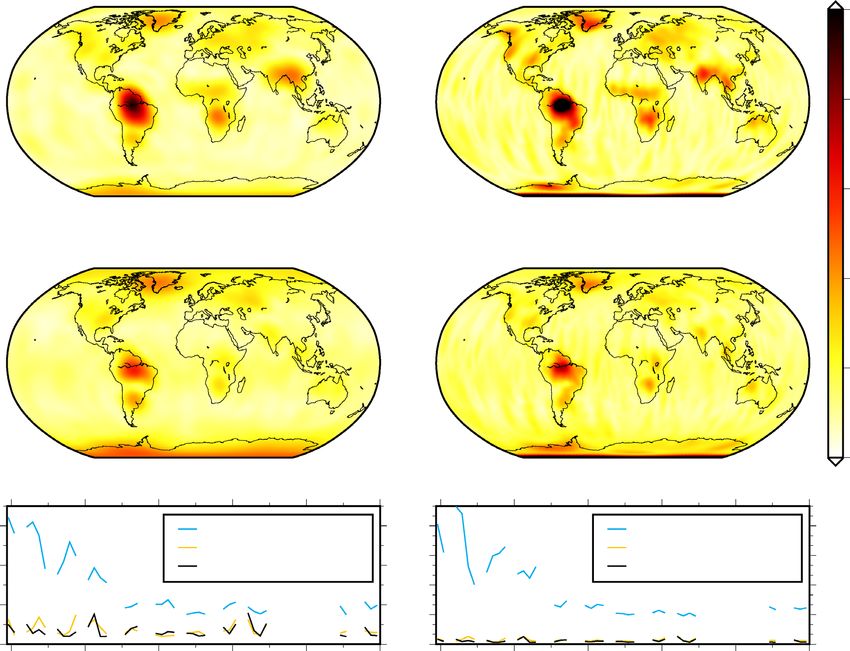
www.nature.com/scientificreports/
June 2017. However, the high accuracy of the GRACE solutions is due to the ultra-precise inter-satellite ranging
system, while with SLR and Swarm, the gravity field solutions can only be retrieved from the tracking of the
spacecraft orbit perturbations, inevitably resulting in lower spatial resolution. In the case of Swarm, the monthly
gravity fields are limited to spherical harmonic degree and order (d/o) of about 12, corresponding to a spatial
resolution of 3000–4000 km.
Previous GRACE and modelling studies have shown that the observed mass change in the cryosphere, hydro-
sphere and oceans can be, to a large extent, explained through a number of modes that represent the temporal
evolution of spatially coherent patterns29–31. This fact has been exploited in signal separation by Refs. 3,32–34, who
identified ENSO events in terrestrial water storage changes. Reference26 consequently employed it for recon-
structing pre-GRACE ice mass changes by combining SLR and Doppler Orbitography and Radiopositioning
Integrated by Satellite (DORIS) with spatial modes from GRACE.
Reference27 provided a comprehensive description of the quality of the gravity recovery approach using
Swarm, proving that its accuracy is comparable to Swarm gravity models delivered by others. References27
and35 both compare the Swarm solutions of different institutes [Astronomical Institute of the University of Bern
(AIUB), Astronomical Institute of the Czech Academy of Science (ASU), Institute of Geodesy (IfG) of the Graz
Universtity of Technology, Institute of Geodesy and Geoinformation (IGG) of the University of Bonn, Ohio State
University (OSU)] and conclude that spherical harmonic degrees higher than 12 should not be used to derive
geophysical signals. In this work, we use the approach of Ref.27 and focus on improving the spatial resolution of
the monthly Swarm models (which are derived up to d/o 40) while ingesting some a-priori information from the
GRACE period. Here, Swarm GNSS-tracking data during December 2013 to December 2018 have been used to
retrieve the temporal evolution of three leading spatial modes, which were derived from GRACE during April
2002 to June 2017. One has to keep in mind that the gravity fields reconstructed in this way are spatially con-
strained by the number of the leading GRACE modes. We evaluate the impact of these constraints by comparing
the monthly Swarm-only solutions and the reconstructed Swarm solutions to the monthly GRACE solutions
during the GRACE-Swarm overlap period. The comparisons are conducted each for a maximum d/o of 12 and
40. In this way, we investigate both the common Swarm resolution and also the actual available resolution, which
mostly contains noise and is thus in general not used (see Swarm Data in the Supplement, Refs.27 and35). We
furthermore validate our results by comparisons to vertical deformations from Global Positioning System (GPS)
and through evaluating range residuals from SLR.
This article is organized as follows: in the following section we describe the time-variable Swarm gravity
fields alongside an error assessment that we obtain from projecting monthly Swarm-only gravity fi elds27 onto
the spatial modes from GRACE. We consider two variants of the reconstruction approach: in the first one, the
entire observed mass change signal is decomposed and projected; in the second variant, a deterministic signal
model is first estimated from the GRACE data, then removed prior to decomposition and ingesting Swarm data,
before subsequently being restored. This can be viewed as combining the GRACE interpolation approach with
the Swarm reconstruction method. We furthermore show comparisons to GPS data and residuals from SLR data.
This is followed by a conclusion and the explanation of our methods.
Time‑variable gravity from Swarm
Monthly Swarm reconstructions. We have reconstructed monthly Swarm geopotential solutions and
surface mass change maps (measured in e.w.h., equivalent water height) from December 2013 to December
2018 using principal component analysis ( PCA36). PCA decomposes the time series of GRACE e.w.h. maps into
orthogonal spatial patterns, each scaled by uncorrelated time series. We utilize the GRACE-derived patterns
in order to represent two variants of the monthly Swarm solutions, referred to as (1) “Swarm reconstruction”
and (2) “Swarm reconstructionresidual ” [see explanation in Methods; if not mentioned explicitly, the results are
shown for the Swarm reconstruction (1)]. As an example, Fig. 1 shows monthly surface mass change maps
for March 2016 from GRACE (top), Swarm-only (center), and Swarm projected to the leading three GRACE-
modes (bottom), each for d/o 12 (left column) and for d/o 40 (right column). The low-degree solution shows
that Swarm-only gravity recovery (Fig. 1c) is able to capture some major patterns of the more precise GRACE
solution (Fig. 1a), but at monthly time-scale noise is ubiquitous. The Swarm reconstruction (Fig. 1e) constrained
by the GRACE spatial patterns is closer to the GRACE monthly solution, with a global root mean square error
(RMSE) of 0.022 m compared to the Swarm-only solution (RMSE 0.092 m). The improvement through the
reconstruction approach is even more striking when we compare d/o 40 solutions (Fig. 1b,d,f); the Swarm-only
solution contains mostly noise (RMSE 0.39 m), while the reconstructed field is very similar to the GRACE solu-
tion (RMSE 0.035 m). For the selected month, the Swarm reconstructionresidual variant shows a slightly larger
RMSE of 0.035 m for d/o 12 and a slightly lower RMSE of 0.030 m for d/o 40, as compared to the Swarm recon-
struction, based on the full signal.
Figure 2 provides an assessment of the errors of the method proposed here compared to GRACE. The maps
in Fig. 2a,b visualize the spatial error of the Swarm reconstruction, while Fig. 2c,d depict the error of the
reconstructedresidual solution. Errors are below 10 cm for most regions. Largest RMS errors are found in the
Amazon basin, where the large hydrological signal can neither be fully captured by Swarm nor fully represented
in three modes. Moreover, climate phenomena like El Niño and La Niña lead to propagating mass change that
also cannot be explained with only three modes (e.g., drought conditions in Northern South America towards
the end of 2015). The degree and order 12 and 40 error maps appear broadly similar, with larger errors for higher
degrees. Furthermore, the Swarm reconstructionresidual variant is comparable to the Swarm reconstruction solu-
tion, with, in general, slightly smaller RMSE values over land and slightly larger RMSE values over the ocean and
Antarctica. When we assess the global mean RMSE as a function of time (Fig. 2e,f) the d/o 40 solutions again
exhibit larger errors, in particular the Swarm-only solution (0.29–1.39 m). The reconstruction method reduces
Scientific Reports | (2021) 11:1117 | https://doi.org/10.1038/s41598-020-80752-w 2
Vol:.(1234567890)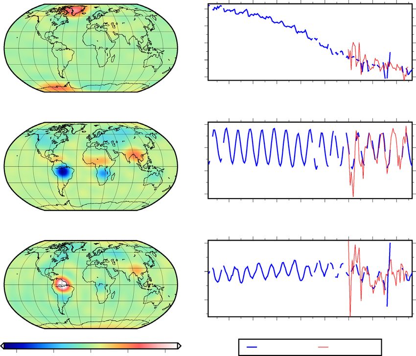
www.nature.com/scientificreports/
d/o 12 d/o 40
a b
GRACE
c d
SH solution
Swarm
e
Reconstruction
f
Swarm
−0.3 −0.2 −0.1 0.0 0.1 0.2 0.3
EWH [m]
Figure 1. March 2016 e.w.h. surface mass change map. Left: d/o 12, right: d/o 40. (a,b) From original GRACE
gravity field. (c,d) From Swarm-only gravity field27. (e,f) Reconstruction from monthly Swarm solutions using
three GRACE EOFs.
the errors significantly (0.025–0.085 m ). Both reconstruction variants show a similar performance with the
Swarm reconstructionresidual variant performing better towards the beginning. The large errors observed at the
start of the Swarm mission can be attributed mainly to higher ionospheric activity during 2014 and 2015. This
affected the performance of Swarm GNSS receivers37, an effect which was mitigated through receiver updates
hase38. The reconstruction is much less affected by ionospheric disturbances as compared
in the early mission p
to the monthly Swarm-only solutions.
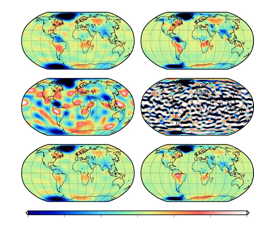
Basin averages. In order to assess the impact of the new approach for typical regional applications, we here
compare area-mean mass changes (in terms of e.w.h.) for basins of various size. Figure 3 shows basin averages
(for the locations, see Fig. 4) for the Antarctic ice sheet, the Amazon basin, the Mississippi basin, the Greenland
ice sheet and the Ganges basin derived from GRACE, Swarm-only and the Swarm reconstruction for d/o 12
and 40. Tables 1 and 2 give an overview of trend and RMSE estimates and also include a six-parameter GRACE
model (constant, trend, and annual and semiannual terms).
The first observation from Tables 1 and 2 is that, during the Swarm time frame considered here, the monthly
GRACE-derived mass anomalies reveal a quite regular behaviour for all regions considered, without larger (e.g.
ENSO-related) temporal anomalies and without trend changes or similar obvious interannual changes. The
GRACE six-parameter signal model follows the monthly GRACE solution within RMSE 2–8 cm, which is quite
moderate when compared to ENSO years. It is thus not surprising that this simple GRACE-based prediction
model already provides a good fit, however this is obviously due to the low variability in the considered time
frame and therefore cannot invalidate methods that rely on other data such as Swarm.
Trends derived from a 4-year period cannot provide significance for assessing geophysical processes, but they
can be compared to each other. We notice, e.g., that for the Amazon basin the GRACE trend within the Swarm
period does not fit well to the overall GRACE trend (which one would have to use when relying on GRACE
Scientific Reports | (2021) 11:1117 | https://doi.org/10.1038/s41598-020-80752-w 3
Vol.:(0123456789)www.nature.com/scientificreports/
d/o 12 d/o 40
Reconstruction vs. GRACE Reconstruction vs. GRACE
Spatial RMSE a b 0.15
0.12
0.09
EWH [m]
ReconstructionResidual vs. GRACE ReconstructionResidual vs. GRACE
c d 0.06
Spatial RMSE
0.03
0.00
e f
Temporal RMSE
[m] [m]
0.3 Swarm−only vs. GRACE 1.2 Swarm−only vs. GRACE
Rec vs. GRACE Rec vs. GRACE
0.9
0.2 RecResidual vs. GRACE RecResidual vs. GRACE
0.6
0.1
0.3
0.0 0.0
2014 2015 2016 2017 2018 2019 2014 2015 2016 2017 2018 2019
Figure 2. Spatial (a–d) and temporal (e, f) RMS errors of the Swarm reconstructed(residual) solution with
respect to GRACE.
interpolation) while for other regions the overall GRACE trend represents a good predictor for the Swarm period.
Again, this is due to only very moderate interannual variability in this timeframe. We notice that trends from
a Swarm-only monthly solution are generally larger as compared to the reconstruction approach, which is in
line with the methodology. We find that Swarm-only trends appear unrealistically large for the Antarctica and
Amazon regions, in particular for d/o 40, while all other approaches including the reconstructions fit to GRACE
trends. Results are diverse for the smaller regions.
As for the RMSE with respect to the monthly GRACE solution, the Swarm-monthly solutions generally
shows the largest misfit, followed by the Swarm reconstruction and then the Swarm reconstructionresidual with
removing-restoring GRACE trends. This is particularly striking for the d/o 40 comparisons where the latter
approach indeed outperforms the GRACE 6-parameter model in almost all regions and sub-intervals. This is
encouraging, but it may be expected due to the mentioned regular behaviour of mass change during the time
frame. It is also worth noting that the Swarm reconstruction without making use of GRACE-trends is much
closer to GRACE as compared to the Swarm-monthly result.
For the entire Antarctic ice sheet, GRACE shows a mass loss until mid-2016. Afterwards, the time series
shows a slight mass gain until November 2016, followed by a drop of approximately 20 cm. This drop is likely
an artifact due to the poorer quality of GRACE data caused by the lack of accelerometer data from GRACE B
for this period39 (in November 2016 the GRACE B accelerometer had been switched off for the first time to save
battery power and non-gravitational accelerations measured onboard GRACE A were transplanted to GRACE
B). This affects the Antarctic regions in particular, as can be seen in the time series as well as in Figs. S2.1
and S2.2 of the Supplement. For this reason, we only consider the time from 2013-12 to 2016-08 for the Antarc-
tic ice sheet, except if stated otherwise. The d/o 40 GRACE solution that we show here points to a mass loss of
145 Gtyr−1 (corresponding to − 0.01myr−1 mass loss in the Antarctic or 0.4mmyr−1 global mean sea level rise)
within December 2013 to August 2016, which is in the same order of magnitude as the 178Gtyr−1 that Ref.2 find
from combining GRACE and Cryosat-2 data for a longer time span (January 2011–June 2017). These rates are
predominately driven by melting glaciers in West Antarctica and the Antarctic peninsula, while the East Ant-
arctic ice sheet appears more stable. As expected, the monthly Swarm-only solutions suffer from considerable
noise, in particular in the beginning. However, for d/o 12, the RMSE between GRACE and Swarm is reduced
Scientific Reports | (2021) 11:1117 | https://doi.org/10.1038/s41598-020-80752-w 4
Vol:.(1234567890)www.nature.com/scientificreports/
0.4 0.4
a RMSEGS: 0.131m b RMSEGS: 0.129m
RMSEGR: 0.064m RMSEGR: 0.072m
Antarctica
0.2 0.2
(12.8 e6 km2)
ewh [m]
ewh [m]
0.0 0.0
−0.2 −0.2
−0.4 −0.4
2014 2015 2016 2017 2018 2019 2014 2015 2016 2017 2018 2019
0.4 0.4
c RMSEGS: 0.096m d RMSEGS: 0.126 m
RMSEGR: 0.110m RMSEGR: 0.113m
0.2 0.2
Amazon
(5.9 e6 km2)
ewh [m]
ewh [m]
0.0 0.0
−0.2 −0.2
−0.4 −0.4
2014 2015 2016 2017 2018 2019 2014 2015 2016 2017 2018 2019
0.4 0.4
e RMSEGS: 0.093m f RMSEGS: 0.106m
Mississippi
RMSEGR: 0.038m RMSEGR: 0.043m
0.2 0.2
(3.2 e6 km2)
ewh [m]
ewh [m]
0.0 0.0
−0.2 −0.2
−0.4 −0.4
2014 2015 2016 2017 2018 2019 2014 2015 2016 2017 2018 2019
0.4 0.4
g RMSEGS: 0.130m h RMSEGS: 0.120m
RMSEGR: 0.070m RMSEGR: 0.069m
Greenland
0.2 0.2
(2.2 e6 km2)
ewh [m]
ewh [m]
0.0 0.0
−0.2 −0.2
−0.4 −0.4
2014 2015 2016 2017 2018 2019 2014 2015 2016 2017 2018 2019
0.8 0.8
i RMSEGS: 0.167m j RMSEGS: 0.449m
RMSEGR: 0.069m RMSEGR: 0.092m
0.4 0.4
Ganges
(1.0 e6 km2)
ewh [m]
ewh [m]
0.0 0.0
−0.4 −0.4
−0.8 −0.8
2014 2015 2016 2017 2018 2019 2014 2015 2016 2017 2018 2019
GRACE Swarm Reconstruction
ErrorReconstruction
Figure 3. Basin averages for different regions expressed in meter of e.w.h. The original GRACE solution, the
original Swarm-only solution, as well as the reconstructed gravity field are shown. Left: d/o 12, right: d/o 40.
The error of the reconstruction is indicated in yellow as computed by Eq. (6). The grey bars in each plot indicate
months with no GRACE and GRACE-FO data. RMSEGS indicates the RMSE of Swarm w.r.t. GRACE, while
RMSEGR refers to the RMSE of the reconstruction approach w.r.t. GRACE. All RMSE values are related to the
overlapping GRACE and Swarm period (December 2013–June 2017).
Scientific Reports | (2021) 11:1117 | https://doi.org/10.1038/s41598-020-80752-w 5
Vol.:(0123456789)www.nature.com/scientificreports/
30
Vertical displacements (mm)
Vertical displacements (mm)
Mi: OKBF 30
Gr: GROK Gr: HJOR
Vertical displacements (mm)
40
20
20 20
10
10
0
0
0
-20
-10 -10
-40
2014 2016 2018 2020 2014 2016 2018 2020 2014 2016 2018 2020
Time (years) Time (years) Time (years)
Gr GRACE Swarm
GROK
GPS Swarm-reconstruction
HJOR Swarm-reconstructionresiduals
Mi
OKBF Ga CHLM
SNDL 60 Ga: CHLM
Vertical displacements (mm)
40
selected basins
GPS stations Am PAIT 20
0
-20
WHTM
An 2014 2016 2018 2020
Time (years)
40 40 40
Ga: SNDL
Vertical displacements (mm)
Vertical displacements (mm)
An: WHTM Am: PAIT
Vertical displacements (mm)
30
20
20 20
10
0
0 0
-20 -10
-20 -20
-40
2014 2016 2018 2020 2014 2016 2018 2020 2014 2016 2018 2020
Time (years) Time (years) Time (years)
Figure 4. Study regions. An: Antarctica, Am: Amazon, Mi: Mississippi, Gr: Greenland, Ga: Ganges. For each
basin, 4 GPS stations were randomly chosen and analyzed. Time series plots present the vertical displacements
for individual stations estimated from: Swarm reconstruction (yellow), Swarm reconstructionresidual (black),
Swarm-only (blue), GRACE (red) and GPS (gray). Remaining stations are included in the supplementary
materials. Stations shown at the charts are marked.
from 0.14 m (monthly Swarm-only solution) to 0.05 m when we use the reconstructed solution (or 0.05 m for
Swarm reconstructionresidual). We find that the trend from the reconstructed Swarm solution (− 0.01myr−1 for d/o
12) over the time span December 2013–June 2017 is the same as the GRACE trend. After the end of the GRACE
lifetime (2017-06 to 2018-12), the Swarm solutions agree with each other by 0.04 m (d/o 12) and 0.035 m (d/o 40).
For the Amazon basin, GRACE exhibits a large seasonal signal overlaid by a declining trend in the years
2015 and 2016, which reverses in 2017. This is likely due to the 2015–2016 drought caused by a strong El Niño40.
From comparing GRACE and GRACE-FO in 2017-2019, we conclude that there is no significant trend in the
GRACE gap. All Swarm solutions appear to follow GRACE and GRACE-FO well after 2015 (monthly Swarm-
only solutions: RMSE 0.08 m for d/o 12 and d/o 40; reconstruction: RMSE 0.07 m for d/o 12 and RMSE 0.10 m
for d/o 40; reconstructionresidual : RMSE 0.08 m for d/o 12 and d/o 40), and they confirm the reversal in 2017 as
well as a stable development after 2017. Here, the reconstruction does not significantly improve over the monthly
Swarm-only solutions, which most likely can be explained by the El Niño not being represented in the first three
EOFs. The Swarm-only and Swarm-reconstructed solutions agree with each other at the level of RMSE 0.06 m
for d/o 12 and 0.08 m for d/o 40 after the end of GRACE (from 2017-06 to 2018-12). They appear able to close
the gap between GRACE and GRACE-FO well.
In the Mississippi basin, GRACE detects strong annual water storage changes with a positive trend (0.01 myr−1
for d/o 12 and d/o 40). After GRACE, the positive trend is still confirmed by GRACE-FO. Ref.41 suggests that the
largest mass changes in this heavily managed area are due to soil moisture and groundwater changes including
withdrawals, followed by relatively small variations in snow depth. For both d/o 12 and d/o 40, the monthly
Scientific Reports | (2021) 11:1117 | https://doi.org/10.1038/s41598-020-80752-w 6
Vol:.(1234567890)www.nature.com/scientificreports/
Antarctica Amazon Mississippi Greenland Ganges
Trend GRACEreal − 0.01a (− 0.01b) − 0.04 (− 0.02) 0.01 (0.01) − 0.04 (− 0.03) − 0.02 (− 0.02)
Trend GRACEsignal − 0.01 (−0.01) 0.00 (0.00) 0.00 (0.00) − 0.05 (−0.05) 0.00 (0.00)
Trend Swarm-only − 0.05 (0.03) − 0.06 (− 0.02) 0.01 (0.01) − 0.03 (− 0.04) − 0.01 (− 0.02)
Trend Swarm-rec − 0.01 (0.00) − 0.07 (0.00) − 0.01 (0.00) − 0.04 (− 0.01) 0.01 (0.00)
Trend Swarm-recresidual − 0.02 (0.02) 0.00 (0.02) 0.00 (− 0.01) − 0.05 (− 0.05) − 0.01 (0.00)
RMSE GRACEsignal versus GRACEreal 0.07 (0.08) 0.07 (0.08) 0.02 (0.02) 0.06 (0.06) 0.03 (0.03)
RMSE Swarm-only versus GRACEreal 0.13 (0.08) 0.10 (0.08) 0.09 (0.04) 0.13 (0.08) 0.17 (0.13)
RMSE Swarm-rec versus GRACEreal 0.06 (0.07) 0.11 (0.07) 0.04 (0.03) 0.07 (0.05) 0.07 (0.06)
RMSE Swarm-recresidual versus GRACEreal 0.08 (0.07) 0.07 (0.08) 0.04 (0.03) 0.08 (0.06) 0.04 (0.03)
RMS(Swarm-only-Swarm-rec)c 0.04 0.06 0.06 0.07 0.09
RMS(Swarm-only-Swarm-recresidual)c 0.02 0.06 0.08 0.06 0.08
Table 1. Trends (myr−1), RMSE (m) and RMS (m) for the d/o 12 solutions in our study regions. The
following cases are investigated: (1) the monthly ITSG-Grace2018 solution (GRACEreal), (2) the 6-parameter
signal model (constant+trend+(semi-)annual) of the monthly ITSG-Grace2018 solution (GRACEsignal ),
(3) the monthly Swarm-only solution, (4) the Swarm-reconstructed solution (Swarm-rec), (5) the Swarm-
reconstructed solution, which is computed on the basis of Swarm and GRACE residuals (Swarm-recresidual ).
RMSE values are all computed w.r.t. GRACEreal. Considered time periods: a 2013-12 to 2017-06: overlapping
GRACE/Swarm period. This period is shown in the first column of each region in the upper part of the table.
b
2015-01 to 2017-06: as the Swarm-only solutions suffer from ionospheric disturbances in the early phase of
the mission, the values in brackets are related to a shorter period. c 2017-07 to 2018-12: in the lower part of the
table, the RMS of Swarm-only minus Swarm-reconstructed(residual) after the end of GRACE is shown.
Antarctica Amazon Mississippi Greenland Ganges
Trend GRACEreal − 0.01a (− 0.01b) − 0.04 (− 0.03) 0.01 (0.01) − 0.04 (− 0.03) − 0.03 (− 0.03)
Trend GRACEsignal − 0.01 (− 0.01) 0.00 (0.00) 0.00 (0.00) − 0.05 (− 0.05) − 0.01 (−0.01)
Trend Swarm-only − 0.05 (0.04) − 0.01 (− 0.05) − 0.03 (− 0.01) − 0.03 (− 0.03) 0.02 (− 0.01)
Trend Swarm-rec − 0.02 (0.01) − 0.06 (0.01) − 0.01 (0.00) − 0.05 (− 0.01) 0.02 (0.00)
Trend Swarm-recresidual − 0.01 (0.01) 0.00 (0.01) 0.00 (0.00) − 0.06 (− 0.06) − 0.01 (0.00)
RMSE GRACEsignal versus GRACEreal 0.06 (0.08) 0.08 (0.08) 0.02 (0.02) 0.06 (0.06) 0.04 (0.04)
RMSE Swarm-only versus GRACEreal 0.13 (0.08) 0.13 (0.08) 0.11 (0.08) 0.12 (0.08) 0.45 (0.24)
RMSE Swarm-rec versus GRACEreal 0.07 (0.08) 0.11 (0.10) 0.04 (0.03) 0.07 (0.05) 0.09 (0.07)
RMSE Swarm-recresidual versus GRACEreal 0.06 (0.07) 0.08 (0.08) 0.02 (0.02) 0.06 (0.04) 0.04 (0.04)
RMS(Swarm-only-Swarm-rec)c 0.04 0.08 0.09 0.07 0.18
RMS(Swarm-only-Swarm-recresidual)c 0.03 0.06 0.11 0.08 0.18
Table 2. Trends (myr−1), RMSE (m) and RMS (m) for the d/o 40 solutions in our study regions. The
following cases are investigated: (1) the monthly ITSG-Grace2018 solution (GRACEreal), (2) the 6-parameter
signal model (constant+trend+(semi-)annual) of the monthly ITSG-Grace2018 solution (GRACEsignal ),
(3) the monthly Swarm-only solution, (4) the Swarm-reconstructed solution (Swarm-rec), (5) the Swarm-
reconstructed solution, which is computed on the basis of Swarm and GRACE residuals (Swarm-recresidual ).
RMSE values are all computed w.r.t. GRACEreal. Considered time periods: a 2013-12 to 2017-06: overlapping
GRACE/Swarm period. This period is shown in the first column of each region in the upper part of the table.
b
2015-01 to 2017-06: as the Swarm-only solutions suffer from ionospheric disturbances in the early phase of
the mission, the values in brackets are related to a shorter period. c 2017-07 to 2018-12: in the lower part of the
table, the RMS of Swarm-only minus Swarm-reconstructed(residual) after the end of GRACE is shown.
Swarm-only solution captures the seasonal signal well, but it does not see the positive trend for d/o 40. The noise
of the monthly Swarm-only solutions (0.09 and 0.11 m e.w.h., respectively) can be strongly mitigated via the
constrained reconstruction (0.04 m for both, d/o 12 and 40) or the reconstructionresidual variant (0.04 m for d/o
12 and 0.02 m for d/o 40). In particular after 2014, the reconstruction represents the GRACE solution very well.
After the end of GRACE, we see a continuation of the annual signal with unchanged amplitude.
For the Greenland ice sheet, we find a dominating melt-related trend with seasonal amplitudes of about
1.5 cm. Interestingly, the melting seems to decelerate when we look at GRACE and GRACE-FO from 2017-2019.
For the d/o 12 solutions, we find a trend of − 0.04 myr−1 for GRACE, − 0.03 myr−1 for the monthly Swarm-only
solution, − 0.04 myr−1 for the reconstruction and − 0.05 myr−1 for the reconstructionresidual (for the existing
GRACE months from December 2013 to June 2017). After 2016, both Swarm solutions follow the seasonal pat-
tern in GRACE mass solutions quite closely. They do not suggest a further acceleration after GRACE’s lifetime.
Scientific Reports | (2021) 11:1117 | https://doi.org/10.1038/s41598-020-80752-w 7
Vol.:(0123456789)www.nature.com/scientificreports/
Gradually, the noise with respect to GRACE is reduced and both Swarm solutions converge towards each other.
After the end of GRACE, there is a drop in the Swarm reconstructed solution, while the Swarm-only solution
is closer to GRACE. This discrepancy leads to an RMS (between the Swarm-only and the Swam reconstruction
solution) of 0.07 m for both d/o 12 and d/o 40 from 2016-07 to 2018-12. In general, the signal-to-noise ratio in
Greenland is quite low, as can be seen in Fig. 3.
The Ganges basin is the smallest study region considered here (approx. 1100 km × 900 km ), even though
our results suggest that future work could concentrate on smaller basins. Apart from the seasonal signal in
the GRACE data, one can see a slight decline of total water storage in the GRACE-FO era. For example, Ref.42
and43 describe interannual water storage variability to human water usage, extreme precipitation (floods and
droughts) and large-scale ocean-atmospheric interactions such as El Niño and Indian Ocean Dipole, yet these
are all dwarfed by the huge seasonal signal. We find that for d/o 12, the monthly Swarm-only solution shows
an RMSE of 0.17 m with respect to GRACE, while the Swarm reconstruction has a much lower RMSE of 0.07 m
and 0.04 m for the reconstructionresidual . The monthly Swarm-only solution for up to d/o 40 exhibits large noise
(RMSE 0.45 m ) and should not be used, while the reconstruction is closer to GRACE (RMSE 0.09 m ). The
Swarm-only and Swarm-reconstructed solutions agree at the level of RMSE 0.09 m for d/o 12 and RMSE 0.18 m
for d/o 40 after the end of GRACE, and they seem to extend the time series without noticeable outliers (except
for monthly d/o 40 data).
All trend and RMSE values are summarized in Tables 1 and 2. A common approach to bridge the GRACE
gaps is to interpolate or extrapolate previous and subsequent GRACE solutions. However, it can be argued that
the skill of such simple extrapolation approaches inevitably depends on how “regular” the true surface mass field
evolves in time, and that scientifically meaningful results are often related to anomalous or episodic events. On
the basis of comparisons to GRACE-derived basin averages, our findings are that monthly Swarm reconstructions
should generally be preferred to a simple six-parameter GRACE model (constant, trend, annual and semiannual
terms), although we admit that the simple model, in certain situations, is sufficient. A detailed analysis can be
found in Section S4 of the Supplement.
Validation with GPS. In order to validate the new approach with independent data, we analyze time
series from twenty globally distributed GPS (Global Positioning System) sites. Vertical GPS displacements were
pre-processed and corrected for non-tidal atmospheric, non-tidal oceanic and post-glacial rebound effects, as
described in the Data section of the Supplement. Mass redistribution estimates derived from GRACE, Swarm-
only, Swarm-reconstructed and Swarm-reconstructedresidual fields of maximum d/o 12 were converted to vertical
deformation using elastic loading theory (Fig. 4). Subsequently, we derived linear trends and annual amplitudes
from daily GPS displacements, GPS displacements averaged to monthly time scale, and displacements estimated
for GRACE, Swarm-only, Swarm-reconstructed and Swarm-reconstructedresidual data.
We find that both Swarm-reconstructed and GRACE-predicted displacements reproduce well inter-annual
signals observed by GPS, while the fits for trends and at the annual timescale are moderate. Inter-annual varia-
tions are large in particular for the Amazon, as noticed by GPS, and they are captured by GRACE and Swarm-
reconstructions. Similarly we find a good agreement at interannual timescales for the Mississippi basin where the
hydrological signals are also large. GPS uplift or subsidence trends which may be caused, next to mass loading, by
a plethora of other geophysical or anthropogenic effects are difficult to compare. At the annual timescale no clear
picture emerges: gravity solutions from the Swarm reconstruction approach seem to outperform monthly Swarm-
only solution for some regions with large signal while for others the Swarm-only monthly solutions appear closer
to GPS. The Swarm-reconstructedresidual variant, which is applied in remove-restore mode, will provide fits very
close to the GRACE-predicted loading and thus performs well where we know, from other studies, that GRACE
fits well to GPS; yet neither Swarm-only nor Swarm reconstructed solutions appear to fit GPS worse.
Validation with satellite laser ranging (SLR). Another way of validating the global gravity solu-
tions is by assessing how well they would allow the prediction of the orbits of other satellites. Here, we use the
Swarm-derived gravity fields for computing post-fit satellite laser ranging (SLR) range residuals to five SLR
satellites; Lageos 1 (altitude 5860 km), Lageos 2 (altitude 5620 km), Ajisai (altitude 1490 km), Starlette (altitude
800 km−1100 km) and Stella (altitude 810 km). Lageos data is processed in orbit arcs of 10 days, while for Ajisai,
Starlette and Stella 3-day arcs are chosen due to limitations in modeling the atmospheric d rag44.
Figure 5 shows the residuals computed with (a) monthly Swarm-only gravity fields and (b) the reconstruction
approach. In both cases, the time-variable gravity fields are truncated at d/o 12 and the same static background
model45 has been applied for d/o 13–120. As already mentioned, the quality of the monthly Swarm-only solutions
is affected by ionospheric disturbances in 2014 and 201537, which can clearly be seen in Fig. 5a. SLR observations
form Ajisai, Stella and Starlette do not match the Swarm-only gravity field during the beginning of the Swarm
mission, leading to residuals of several decimeters. The SLR residuals reveal (again) that the reconstruction
approach does not seem to be affected by the ionospheric disturbances. Starting in 2016, the residuals of both
approaches get more similar, but those of the reconstruction are still lower. As Lageos 1/2 fly in a higher orbit
than the other three satellites, they are less sensitive to details of the gravity field. Thus, the improvement when
using the Swarm reconstruction can mainly been seen when looking at Ajisai, Stella and Starlette. In summary,
the analysis of SLR range residuals confirms the capability of the reconstruction approach to improve time-
variable gravity fields from Swarm.
Scientific Reports | (2021) 11:1117 | https://doi.org/10.1038/s41598-020-80752-w 8
Vol:.(1234567890)www.nature.com/scientificreports/
SLR residuals from monthly Swarm gravity fields
0.5
a
0.4
0.3
[m]
0.2
0.1
0.0
2014 2015 2016 2017 2018 2019
SLR residuals from monthly reconstruction
0.5
b
0.4
0.3
[m]
0.2
0.1
0.0
2014 2015 2016 2017 2018 2019
Lageos2 Lageos1 Ajisai Stella Starlette
Figure 5. Post-fit range residuals of five SLR satellites. (a) Computed with monthly Swarm-only gravity fields.
(b) Computed with monthly reconstruction.
Conclusions
We find that the Swarm time series have the potential to fill the gap between GRACE and GRACE-FO. They
follow the GRACE solutions well, but show an elevated level of noise as compared to GRACE, as expected. The
two variants of the new reconstruction approach reduce the variance further and improve Swarm results, as
we show during the overlap period with GRACE. Our main result is that for the recent period (mid-2017 til
mid-2018) which is not covered by GRACE, mass change in all major basins occurs quite regularly compared
to earlier GRACE results, as could have been predicted from a climatology. For the Mississippi basin, we find a
RMSE of 0.09 m for the monthly Swarm-only solutions until d/o 12 and 0.04 m for the reconstruction approach.
The improvement becomes even more evident when we consider higher degree solutions: while we suggest that
the monthly d/o 40 Swarm-only solutions should rather not be utilized to full resolution, the reconstruction
provides reasonable results (RMSE Mississippi: 0.11 and 0.04 m). In general, the RMSE with respect to GRACE
appears higher in the early Swarm years because of the strong ionospheric activity that affected Swarm precise
orbit determination.
Global reconstructed maps of equivalent water height are much closer to GRACE as compared to monthly
Swarm maps. For d/o 40, monthly Swarm-only maps have a global RMSE of 1.39 m in the beginning of the
Scientific Reports | (2021) 11:1117 | https://doi.org/10.1038/s41598-020-80752-w 9
Vol.:(0123456789)www.nature.com/scientificreports/
mission, which decreases to 0.29 m. The reconstructed maps have a lower RMSE of 0.08–0.02 m. The reconstruc-
tion approach enables one to derive reasonable monthly maps for d/o 40, something which would not be possible
when relying on the Swarm-only monthly solutions.
An independent validation with five SLR satellites confirms that the reconstruction approach can improve
time-variable gravity fields from Swarm. Furthermore, comparison to GPS vertical displacements suggests that
Swarm-reconstructed deformation fields can cover most of the GPS-observed displacements; relevant for regions
where hydrology-induced deformation dominates other effects that GPS is sensitive to.
In this work we have demonstrated a new alternative to simply extrapolating GRACE results in order to fill
the GRACE-GRACE-FO mission gap. While this was already possible up to d/o 12 with Swarm gravity data,
here we prove that one can achieve higher resolution with a reconstruction approach. Of course this comes at
the expense that we have to prescribe GRACE-derived spatial patterns. However, comparing approaches in the
overlap period suggests that the new approach clearly outperforms Swarm-only monthly solutions at least for
budget studies. We present two variants of the approach: in the first one the entire signal is used in the Principal
Component Analysis, leading to a larger flexibility. In the second variant, the PCA is based on GRACE and Swarm
residuals, resulting in solutions closer to a 6-parameter GRACE signal model. In other words, this can be viewed
as combining GRACE inter-/extrapolation with Swarm analysis of the residual mass fields.
Errors of the reconstruction approach are significantly larger than with GRACE, which was to be expected,
but they are considerably smaller than those from Swarm-only data. Our results show that at least for some
regions the observed signals are significantly larger than the noise, and scientific interpretation of these signals
will provide new insight, in the absence of other methodes.
This work will be valuable for those researchers who have used GRACE results at large-scale or basin-averaged
level in the past, for example in order to close the water balance and resolve for evapotranspiration or evapora-
tion minus p recipitation46–49. Another large field of application is the study of the global sea level budget, where
it is of utmost importance to partition the altimetric sea level change (≈ 3 mmyr−1) into steric and mass-driven
contributions50. It would be important here to establish consistency across the GRACE / GRACE-FO era by
providing a Swarm estimate. Finally, we believe the newly developed Swarm solutions can provide a blueprint for
potential future gaps in the GRACE-FO mission, or between GRACE-FO and a follow-on mission, if required.
They could also be applied with other LEOs in order to reconstruct temporal gravity field variability prior to
the GRACE mission.
Methods
Principal component analysis (PCA). We pursue two variants using a principal component analy-
sis (PCA36) to reconstruct monthly Swarm geopotential solutions: (1) “Swarm reconstruction” and (2)
“Swarm reconstructionresidual ”. For the Swarm reconstruction (1), we represent the monthly GRACE-derived
surface mass changes through a series of m mode time series (ai (t); equals the ith column of A) which each
scale a corresponding spatial pattern, c.f. Eq. (1). We apply PCA to the monthly e.w.h. grids, following Ref.29.
PCA decomposes time series of e.w.h. maps, here collected in the n × m matrix X , with n epochs and the m grid
points,
X = UDVT = AVT , (1)
into uncorrelated temporal modes (the principal components, contained in A = UD, with U being the n × m
matrix of eigenvectors of X T X , and the squared singular values on the diagonal of m × m matrix D) and orthogo-
nal spatial patterns or Empirical Orthogonal Functions, EOFs (eigenvectors vi of XX T ) contained in the m × m
matrix V . The patterns are typically ordered according to how much variability in the original data they explain,
and often few are sufficient to retain the underlying i nformation26. Equation (1) can be recast as
x(t) = v1 a1 (t) + v2 a2 (t) + · · · + vm am (t). (2)
While it is clear that EOF modes and patterns do not necessarily isolate independent physical processes (see
discussion in Ref.32), the method has been proven capable of effectively rejecting GRACE noise and unphysical
stripes29 and identifying correlations of total water storage variability with climate m
odes34,51, whose indicators
are often defined through PCA of meteorological fields.
Here we suggest to utilize a finite combination of GRACE-derived EOF patterns of surface mass variability
in order to represent the monthly Swarm solutions,
l(t) = v1 b1 (t) + v2 b2 (t) + · · · + vm̄ bm̄ (t), (3)
where l(t) contains all gridded e.w.h. values derived from a given Swarm solution for each monthly epoch t. The
terms bi (t) are the Swarm time series that will be multiplied with GRACE patterns and need to be solved for in
a least-squares adjustment. It makes sense to resolve only a reduced number m̄, since Swarm models have less
spatial details. Here, we chose m̄ = 3, which explains ∼ 90% of the signal. The choice of three EOFs is a result of
a global analysis of the RMS of the Swarm reconstruction w.r.t GRACE (as can be seen in Fig. 2 for three EOFs)
and a regional analysis of basin averages of our study regions and additional further regions (see Section S5 of
the Supplement).
The Swarm reconstructionresidual variant (2) works analogously, but is is based on GRACE and Swarm residu-
als. The first step in this approach is to compute a 6-parameter model (constant, trend, annual and semiannual
terms) from the whole GRACE(-FO) and Swarm period, respectively and subtract it from the original data.
The reconstruction, as explained above, is then computed with the residual data. Finally, the GRACE 6-param-
eter model is added back to the solution, which consequently consists of the main GRACE signal with added
Scientific Reports | (2021) 11:1117 | https://doi.org/10.1038/s41598-020-80752-w 10
Vol:.(1234567890)www.nature.com/scientificreports/
a b
EOF1 (73.1%) PC 1
10
0
−10
−20
−30
2004 2006 2008 2010 2012 2014 2016 2018
c d
EOF2 (14.4%) PC 2
10
0
−10
−20
2004 2006 2008 2010 2012 2014 2016 2018
e f
EOF3 (2.8%) PC 3
10
0
−10
2004 2006 2008 2010 2012 2014 2016 2018
GRACE Reconstruction
−30 −15 0 15 30
EWH [mm]
Figure 6. First three dominant orthogonal patterns from monthly GRACE data (left), and corresponding
temporal modes derived from GRACE and from Swarm (right).
deviations computed from GRACE and Swarm residual data. Here, 3 EOFs have also proven to deliver best
results w.r.t. original GRACE data.
Figure 6 shows the first three dominating spatial patterns and corresponding modes from GRACE until d/o
12. The first mode explains 73.1% of the surface mass variability and represents known long-term trends, such
as ice-mass loss over Greenland, Antarctica, and Alaska glaciers due to warming oceans (as already shown by
e.g. Refs.32 or26). The corresponding PC shows an acceleration until 2015, followed by a deceleration towards the
end of GRACE, which continues for GRACE-FO. It should be mentioned that the months from November 2016
to June 2017 are of minor quality, due to missing accelerometer data as can be seen in Fig. S2.1 and S2.2 of the
Supplement39. The second mode (14.4%) captures the large seasonal mass changes in the terrestrial hydrological
cycle, while the third mode, also seasonal, contains only 2.8% of the variability.
Figure 6 also shows the corresponding temporal modes derived from Swarm (in red), which capture the
main signals quite well. An acceleration signal is visible in the first mode which results from the combined
acceleration of mass loss over the large ice shields52; the Swarm mode is noisier but captures the trend well. It
furthermore confirms the deceleration signal after 2015. The second and the third mode in GRACE describe
the annual mass redistribution amplitude and its phase, and they represent inter-annual variability. Apart from
2014, Swarm reproduces those modes well.
Error budget. In this section, we assess the uncertainty of the Swarm reconstruction. The commission error
considers the error between the Swarm reconstruction and the GRACE solution (considered as the truth in the
overlap period), if we use the same number of EOFs for both:
ec (t) = [v1 a1 (t) + v2 a2 (t) + · · · + vm̄ am̄ (t)] − [v1 b1 (t) + v2 b2 (t) + · · · + vm̄ bm̄ (t)]. (4)
The omission error takes into account that we are not able to reconstruct the full number of EOFs for the
reconstruction. We can assess this error by assembling the GRACE signal starting with EOF m̄ + 1 until EOF m:
eo (t) = vm̄+1 am̄+1 (t) + vm̄+2 am̄+2 (t) + · · · + vm am (t). (5)
We describe the total error e(t) as
Scientific Reports | (2021) 11:1117 | https://doi.org/10.1038/s41598-020-80752-w 11
Vol.:(0123456789)www.nature.com/scientificreports/
e(t) = ec2 (t) + eo2 (t). (6)
Received: 27 April 2020; Accepted: 22 December 2020
References
1. Wouters, B., Gardner, A. S. & Moholdt, G. Global glacier mass loss during the GRACE satellite mission (2002–2016). Front. Earth
Sci. 7, 96. https://doi.org/10.3389/feart.2019.00096 (2019).
2. Sasgen, I., Konrad, H., Helm, V. & Grosfeld, K. High-resolution mass trends of the antarctic ice sheet through a spectral combina-
tion of satellite gravimetry and radar altimetry observations. Remote Sens.https://doi.org/10.3390/rs11020144 (2019).
3. Eicker, A., Forootan, E., Springer, A., Longuevergne, L. & Kusche, J. Does GRACE see the terrestrial water cycle “intensifying’’?.
J. Geophys. Res. Atmos. 121, 733–745. https://doi.org/10.1002/2015JD023808 (2016).
4. Scanlon, B. R. et al. Global models underestimate large decadal declining and rising water storage trends relative to GRACE satellite
data. Proc. Natl. Acad. Sci. 115, E1080–E1089. https://doi.org/10.1073/pnas.1704665115 (2018).
5. Reager, J. T., Thomas, B. & Famiglietti, J. S. River basin flood potential inferred using grace gravity observations at several months
lead time. Nat. Geosci. 7, 588–592. https://doi.org/10.1038/NGEO2203 (2014).
6. Thomas, A. C., Reager, J. T., Famiglietti, J. S. & Rodell, M. A GRACE-based water storage deficit approach for hydrological drought
characterization. Geophys. Res. Lett. 41, 1537–1545. https://doi.org/10.1002/2014GL059323 (2014).
7. Gerdener, H., Engels, O. & Kusche, J. A framework for deriving drought indicators from the Gravity Recovery and Climate Experi-
ment (GRACE). Hydrol. Earth Syst. Sci. 24, 227–248. https://doi.org/10.5194/hess-24-227-2020 (2020).
8. Chambers, D. P. & Bonin, J. A. Evaluation of Release-05 GRACE time-variable gravity coefficients over the ocean. Ocean Sci. 8,
859–868. https://doi.org/10.5194/os-8-859-2012 (2012).
9. Rietbroek, R., Brunnabend, S.-E., Kusche, J., Schröter, J. & Dahle, C. Revisiting the contemporary sea-level budget on global and
regional scales. Proc. Natl. Acad. Sci. 113, 1504–1509. https://doi.org/10.1073/pnas.1519132113 (2016).
10. Engels, O., Gunter, B., Riva, R. & Klees, R. Separating geophysical signals using GRACE and high-resolution data: a case study in
Antarctica. Geophys. Res. Lett. 45, 12340–12349. https://doi.org/10.1029/2018GL079670 (2018).
11. Sasgen, I. et al. Altimetry, gravimetry, GPS and viscoelastic modeling data for the joint inversion for glacial isostatic adjustment
in Antarctica (ESA STSE Project REGINA). Earth Syst. Sci. Data 10, 493–523. https://doi.org/10.5194/essd-10-493-2018 (2018).
12. Willen, M. O. et al. Sensitivity of inverse glacial isostatic adjustment estimates over Antarctica. Cryosphere 14, 349–366. https://
doi.org/10.5194/tc-14-349-2020 (2020).
13. de Viron, O., Panet, I., Mikhailov, V., Van Camp, M. & Diament, M. Retrieving earthquake signature in grace gravity solutions.
Geophys. J. Int. 174, 14–20. https://doi.org/10.1111/j.1365-246X.2008.03807.x (2008).
14. Chao, B. F. & Liau, J. R. Gravity changes due to large earthquakes detected in GRACE satellite data via empirical orthogonal func-
tion analysis. J. Geophys. Res. Solid Earth 124, 3024–3035. https://doi.org/10.1029/2018JB016862 (2019).
15. Zaitchik, B. F., Rodell, M. & Reichle, R. H. Assimilation of GRACE terrestrial water storage data into a land surface model: results
for the Mississippi River Basin. J. Hydrometeorol. 9, 535–548. https://doi.org/10.1175/2007JHM951.1 (2008).
16. Eicker, A., Schumacher, M., Kusche, J., Döll, P. & Schmied Müller, H. Calibration/data assimilation approach for integrating GRACE
data into the WaterGAP Global Hydrology Model (WGHM) using an ensemble Kalman Filter: first results. Surv. Geophys. 35,
1285–1309. https://doi.org/10.1007/s10712-014-9309-8 (2014).
17. Humphrey, V. & Gudmundsson, L. GRACE-REC: a reconstruction of climate-driven water storage changes over the last century.
Earth Syst. Sci. Data Discuss. 1–41, 2019. https://doi.org/10.5194/essd-2019-25 (2019).
18. Sun, A. Y. et al. Combining physically based modeling and deep learning for fusing GRACE satellite data: can we learn from
mismatch?. Water Resour. Res. 55, 1179–1195. https://doi.org/10.1029/2018WR023333 (2019).
19. Li, F. et al. Comparison of data-driven techniques to reconstruct (1992–2002) and predict (2017–2018) GRACE-like gridded total
water storage changes using climate inputs. Water Resour. Res.https://doi.org/10.1029/2019WR026551 (2020).
20. Rietbroek, R. et al. Can GPS-derived surface loading bridge a GRACE mission gap?. Surv. Geophys. 35, 1267–1283. https://doi.
org/10.1007/s10712-013-9276-5 (2014).
21. Argus, D. F. et al. Sustained water loss in California’s mountain ranges during severe drought from 2012 to 2015 inferred from
GPS. J. Geophys. Res. Solid Earth 122, 10559–10585. https://doi.org/10.1002/2017JB014424 (2017).
22. Chanard, K., Fleitout, L., Calais, E., Rebischung, P. & Avouac, J.-P. Toward a global horizontal and vertical elastic load deforma-
tion model derived from grace and GNSS station position time series. J. Geophys. Res. Solid Earth 123, 3225–3237. https://doi.
org/10.1002/2017JB015245 (2018).
23. Dong, D., Fang, P., Bock, Y., Cheng, M. & Miyazaki, S. Anatomy of apparent seasonal variations from gps derived site position
time series. J. Geophys. Res.https://doi.org/10.1029/2001JB000573 (2002).
24. Langbein, J. & Svarc, J. L. Evaluation of temporally correlated noise in global navigation satellite system time series: geodetic
monument performance. J. Geophys. Res. Solid Earth 124, 925–942. https://doi.org/10.1029/2018JB016783 (2019).
25. Mémin, A., Boy, J.-P. & Santamaria-Gomez, A. Correcting GPS measurements for non-tidal loading. GPS Solut.https://doi.
org/10.1007/s10291-020-0959-3 (2020).
26. Talpe, M. J. et al. Ice mass change in Greenland and Antarctica between 1993 and 2013 from satellite gravity measurements. J.
Geod. 91, 1283–1298. https://doi.org/10.1007/s00190-017-1025-y (2017).
27. Lück, C., Kusche, J., Rietbroek, R. & Löcher, A. Time-variable gravity fields and ocean mass change from 37 months of kinematic
Swarm orbits. Solid Earth 9, 323–339. https://doi.org/10.5194/se-9-323-2018 (2018).
28. Jäggi, A. et al. Swarm kinematic orbits and gravity fields from 18 months of GPS data. Adv. Space Res. 57, 218–233. https://doi.
org/10.1016/j.asr.2015.10.035 (2016).
29. Schrama, E. J. O., Wouters, B. & Lavallée, D. A. Signal and noise in Gravity Recovery and Climate Experiment (GRACE) observed
surface mass variations. J. Geophys. Res. Solid Earthhttps://doi.org/10.1029/2006JB004882 (2007).
30. Wouters, B. & Schrama, E. J. O. Improved accuracy of GRACE gravity solutions through empirical orthogonal function filtering
of spherical harmonics. Geophys. Res. Lett.https://doi.org/10.1029/2007GL032098 (2007).
31. Rangelova, E., Van der Wal, W., Braun, A., Sideris, M. G. & Wu, P. Analysis of Gravity Recovery and Climate Experiment time-
variable mass redistribution signals over North America by means of principal component analysis. J. Geophys. Res.https://doi.
org/10.1029/2006JF000615 (2007).
32. Forootan, E. & Kusche, J. Separation of global time-variable gravity signals into maximally independent components. J. Geod. 86,
477–497. https://doi.org/10.1007/s00190-011-0532-5 (2012).
33. Phillips, T., Nerem, R. S., Fox-Kemper, B., Famiglietti, J. S. & Rajagopalan, B. The influence of enso on global terrestrial water
storage using grace. Geophys. Res. Lett. 39, L16705. https://doi.org/10.1029/2012GL052495 (2012) (7pp).
Scientific Reports | (2021) 11:1117 | https://doi.org/10.1038/s41598-020-80752-w 12
Vol:.(1234567890)www.nature.com/scientificreports/
34. de Linage, C., Kim, H., Famiglietti, J. S. & Yu, J.-Y. Impact of Pacific and Atlantic sea surface temperatures on interannual and
decadal variations of GRACE land water storage in tropical South America. J. Geophys. Res. Atmos. 118, 10811–10829. https://doi.
org/10.1002/jgrd.50820(2013).
35. Encarnação De Teixeira, J. et al. Description of the multi-approach gravity field models from Swarm GPS data. Earth Syst. Sci.
Data 12, 1385–1417. https://doi.org/10.5194/essd-12-1385-2020 (2020).
36. Preisendorfer, R. W. & Mobley, C. Principal Component Analysis in Meteorology and Oceanography (Elsevier, Amsterdam, 1988).
37. Schreiter, L., Arnold, D., Sterken, V. & Jäggi, A. Mitigation of ionospheric signatures in swarm GPS gravity field estimation using
weighting strategies. Annales Geophysicae 37, 111–127. https://doi.org/10.5194/angeo-37-111-2019 (2019).
38. Dahle, C., Arnold, D. & Jäggi, A. Impact of tracking loop settings of the Swarm GPS receiver on gravity field recovery. Adv. Space
Res. 22, 122. https://doi.org/10.1016/j.asr.2017.03.003 (2017).
39. Flechtner, F., Bettadpur, S., Gerhard, K. & Christoph, D. GRACE science data system monthly report. Technical report, GFZ (2017).
40. Jimenez-Munoz, J.-C. et al. Record-breaking warming and extreme drought in the Amazon rainforest during the course of El Niño
2015–2016. Sci. Rep. 22, 6. https://doi.org/10.1038/srep33130 (2016).
41. Rodell, M. et al. Estimating groundwater storage changes in the Mississippi River basin (USA) using GRACE. Hydrogeol. J. 15,
59–166. https://doi.org/10.1007/s10040-006-0103-7 (2007).
42. Shamsudduha, M., Taylor, R. G. & Longuevergne, L. Monitoring groundwater storage changes in the highly seasonal humid tropics:
validation of grace measurements in the Bengal basin. Water Resour. Res.https://doi.org/10.1029/2011WR010993 (2012).
43. Forootan, E., Schumacher, M., Awange, J. L. & Müller, Schmied H. Exploring the influence of precipitation extremes and human
water use on total water storage (TWS) changes in the Ganges–Brahmaputra–Meghna river basin. Water Resour. Res. 52, 2240–
2258. https://doi.org/10.1002/2015WR018113 (2016).
44. Löcher, A. & Kusche, J. A hybrid approach for recovering high-resolution temporal gravity fields from satellite laser ranging. J.
Geod. 95, 6. https://doi.org/10.1007/s00190-020-01460-x (2021).
45. Pail, R., Gruber, T., Fecher, T. & GOCO Project Team. The combined gravity model GOCO05c. GFZ Data Serv.https://doi.
org/10.5880/icgem.2016.003 (2016).
46. Fersch, B. & Kunstmann, H. Atmospheric and terrestrial water budgets: sensitivity and performance of configurations and global
driving data for long term continental scale WRF simulations. Clim. Dyn. 42, 2367–2396. https://doi.org/10.1007/s00382-013-
1915-5 (2013).
47. Oki, T. & Yeh, P.J.-F. Water and Energy Cycles 895–903 (Springer, New York, 2014).
48. Sebastian, D., Pathak, A. & Ghosh, S. Use of atmospheric budget to reduce uncertainty in estimated water availability over South
Asia from Different Reanalyses. Sci. Rep. 6, 29664. https://doi.org/10.1038/srep29664 (2016).
49. Springer, A., Eicker, A., Bettge, A., Kusche, J. & Hense, A. Evaluation of the water cycle in the European COSMO-REA6 reanalysis
using GRACE. Water 9, 289. https://doi.org/10.3390/w9040289 (2017).
50. WCRP Global Sea Level Budget Group. Global sea-level budget 1993-present. Earth Syst. Sci. Data 10, 1551–1590 (2018).
51. de Viron, O., Panet, I. & Diament, M. Extracting low frequency climate signal from GRACE data. eEarth 1, 9–14 (2006).
52. Nerem, R. S. et al. Climate-change driven accelerated sea-level rise detected in the altimeter era. Proc. Natl. Acad. Sci. 115,
2022–2025. https://doi.org/10.1073/pnas.1717312115 (2018).
53. Wessel, P. et al. The generic mapping tools version 6. Geochem. Geophys. Geosyst. 20, 5556–5564. https://doi.org/10.1029/2019G
C008515 (2019).
Acknowledgements
The first author is grateful for financial support by PROMOS. This study is supported by the Priority Program
1788 “Dynamic Earth” of the German Research Foundation (DFG)—FKZ: RI 2657/2-2. Contribution of A.K.
was funded by project under the Ministry of National Defense Republic of Poland Program—Research Grant.
The study is also supported by a grant to the fourth author from the Natural Sciences and Engineering Research
Council (NSERC) of Canada. Thanks to Dr. Anno Löcher for computing the SLR range residuals. All figures
(including those in the Supplement) were generated using GMT software version 6.0.0. (https://www.generic-
mapping-tools.org/)53.
Author contributions
J.K. conceived the experiments, H.M.P.R. conducted most of the experiments, with help from C.L. for Swarm
experiments and A.K. for GPS experiments. All authors analysed the results and reviewed the manuscript.
Funding
Open Access funding enabled and organized by Projekt DEAL.
Competing interests
The authors declare no competing interests.
Additional information
Supplementary Information The online version contains supplementary material availlable at https://doi.
org/10.1038/s41598-020-80752-w.
Correspondence and requests for materials should be addressed to C.L.
Reprints and permissions information is available at www.nature.com/reprints.
Publisher’s note Springer Nature remains neutral with regard to jurisdictional claims in published maps and
institutional affiliations.
Scientific Reports | (2021) 11:1117 | https://doi.org/10.1038/s41598-020-80752-w 13
Vol.:(0123456789)You can also read