Real-time Monte Carlo Denoising with the Neural Bilateral Grid
←
→
Page content transcription
If your browser does not render page correctly, please read the page content below

Eurographics Symposium on Rendering (DL-only Track) (2020)
C. Dachsbacher and M. Pharr (Editors)

     Real-time Monte Carlo Denoising with the Neural Bilateral Grid

                              Xiaoxu Meng1            , Quan Zheng1,2       , Amitabh Varshney1 , Gurprit Singh2 , Matthias Zwicker1
                                                                 1 University  of Maryland, College Park, USA
                                                                2 Max   Planck Institute for Informatics, Germany

         Abstract
         Real-time denoising for Monte Carlo rendering remains a critical challenge with regard to the demanding requirements of both
         high fidelity and low computation time. In this paper, we propose a novel and practical deep learning approach to robustly
         denoise Monte Carlo images rendered at sampling rates as low as a single sample per pixel (1-spp). This causes severe noise,
         and previous techniques strongly compromise final quality to maintain real-time denoising speed. We develop an efficient con-
         volutional neural network architecture to learn to denoise noisy inputs in a data-dependent bilateral space. Our neural network
         learns to generate a guide image for first splatting noisy data into the grid, and then slicing it to read out the denoised data. To
         seamlessly integrate bilateral grids into our trainable denoising pipeline, we leverage a differentiable bilateral grid, called neu-
         ral bilateral grid, which enables end-to-end training. In addition, we also show how we can further improve denoising quality
         using a hierarchy of multi-scale bilateral grids. Our experimental results demonstrate that this approach can robustly denoise
         1-spp noisy input images at real-time frame rates (a few milliseconds per frame). At such low sampling rates, our approach
         outperforms state-of-the-art techniques based on kernel prediction networks both in terms of quality and speed, and it leads to
         significantly improved quality compared to the state-of-the-art feature regression technique.
         CCS Concepts
         • Computing methodologies → Neural networks; Ray tracing;

1. Introduction                                                                             oped denoising networks to predict pixel-centric kernels for fil-
                                                                                            tering, Gharbi et al. [GLA∗ 19] predict sample-centric kernels for
Monte Carlo ray tracing has become the de facto standard in                                 splatting individual rendering samples to pixels. These techniques
movie production for its ability to accurately simulate physics-                            achieve good image quality, yet they have been designed for in-
based global illumination. Large numbers of ray samples, how-                               put images rendered with at least 8 ∼ 16 spp, which currently pre-
ever, have to be invested to obtain noise-free images. This leads                           cludes them from real-time applications. Chaitanya et al. [CKS∗ 17]
to significant computational requirements that have restricted such                         proposed a denoiser for interactive applications that are targeted at
techniques to offline rendering. Therefore, real-time, high-quality                         images rendered with low sampling rates (1 ∼ 4spp). In addition,
Monte Carlo ray tracing has been an elusive goal until now.                                 this technique was later integrated into the NVIDIA OptiX engine
   Currently, two main paths appear most promising to achieve fast                          and it can be considered as the current industry standard for inter-
and noise-free Monte Carlo rendering. The first path is to develop                          active denoising. The approach is based on an autoencoder archi-
ever more powerful processors that are enhanced with ray tracing-                           tecture that is simple enough such that interactive frame rates can
specific functionality, like Nvidia’s RT Cores [Wik18]. While re-                           be maintained. The limited capacity of the neural network, how-
cent progress has been impressive, high quality, real-time render-                          ever, leads to compromised image quality compared to offline tech-
ing without additional post-processing is unlikely to become prac-                          niques. In this paper, we propose a novel deep learning approach
tical in the near future. In addition, adapting existing ray tracing                        to denoise Monte Carlo images rendered with extremely few sam-
software frameworks to new hardware is not an easy task in itself.                          ples. The core idea of our approach is to leverage the neural bilat-
The second path is to generate noise-free images from noisy in-                             eral grid [GCB∗ 17] for denoising. We splat noisy image data into
puts rendered in real-time with very low numbers of ray samples.                            a data-dependent bilateral grid, and the data-dependent mapping of
Since this approach can be implemented as a post-processing mod-                            image pixels into the grid is implemented using a neural network.
ule without significant changes to existing renderers, it has gained                        The intuition is that effective data-dependent splatting into the bi-
overwhelming popularity in industrial production and academic re-                           lateral grid can be learned with a simpler network than denoising
search. The most powerful techniques from recent research on off-                           the image itself, and denoising via the bilateral grid is very fast
line denoising rely on deep convolutional neural networks (CNNs).                           as its complexity does not depend on the support of the resulting
While Bako et al. [BVM∗ 17] and Vogels et al. [VRM∗ 18] devel-                              denoising filter. In practice, our network predicts a guide image to

 c 2020 The Author(s)
Eurographics Proceedings c 2020 The Eurographics Association.
X. Meng et al. / Real-time MC Denoising with the Neural Bilateral Grid

control how image data is splatted into the bilateral grid. In the bi-        lationship between feature buffers and radiance and also achieve
lateral space, splatting samples are fused by simple tent filtering.          excellent denoising performance for off-line rendering.
Because of the low resolution of the grid, this effectively denoises             Following the success of deep neural network in image process-
the data. As a final step, we reuse the guide image from the neural           ing, Kalantari et al. [KBS15] proposed a fully-connected neural
network to extract data from the bilateral grid to reconstruct the de-        network to estimate parameters of bilateral denoising filters. Bako
noised results, which is called slicing. Notably, we implement the            et al. [BVM∗ 17] and Vogels et al. [VRM∗ 18] present a convolu-
bilateral grid as a differentiable component, such that we can seam-          tional architecture to predict per-pixel filtering kernels, whereas
lessly integrate it with the neural network for end-to-end training.          Gharbi et al. [GLA∗ 19] propose to predict kernels on a sample ba-
   In addition, we propose a hierarchy of multi-scale bilateral grids         sis and splat samples onto pixels. In gradient-domain rendering,
that leads to further improvements of denoising quality at a slight           Kettunen et al. [KHL19] developed a convolutional neural network
increase of the computational cost. Finally, to denoise consecutive           for the screened Poisson reconstruction process and achieve a sig-
frames from a video, we apply temporal enhancement steps to en-               nificant quality improvement compared to the original gradient do-
sure temporal stability. Inspired by [KIM∗ 19], we apply temporal             main path tracing [KMA∗ 15]. Recently, generative adversarial ar-
accumulation of consecutive frames in our pipeline to increase ef-            chitectures [XZW∗ 19] were also employed to denoise Monte Carlo
fective sampling rates and suppress temporal artifacts.                       rendering. While the above neural network-based approaches often
                                                                              achieve better denoising performance compared to traditional tech-
   According to comprehensive experiments, our light-weight neu-              niques, they may suffer from high computational costs caused by
ral network leveraging the neural bilateral grid is able to denoise           deep neural network architectures, which may limit them to offline
noisy input frames at real-time frame rates (a few milliseconds per           rendering. In contrast, our neural approach can robustly denoise ill-
frame), and at the same time to provide comparable and even higher            posed noisy input (even with 1-spp) at real-time frame rates.
quality for 1-spp data than the state-of-the-art real-time denoising
approaches. In addition, with a deeper neural network architecture,           Real-time Denoising. Real-time path tracing reconstruction gen-
we can further improve denoising quality while still ensuring in-             erally aims at 1-spp noisy input data to limit computation time,
teractive rates at dozens of frames per second. To summarize, our             which requires powerful post-processing and denoising steps to
approach makes the following contributions:                                   obtain acceptable output images. Many approaches for fast filter-
                                                                              ing have been developed [Bur81, DSHL10, MMBJ17] for exam-
• A novel, practical and robust denoising approach using neural
                                                                              ple based on hierarchical filtering, wavelets, or fast approximations
  networks. Experiments have demonstrated better denoising qual-
                                                                              of the bilateral filter [TM98]. A recent neural network approach
  ity than existing methods at very low sample rates.
                                                                              [CKS∗ 17] based on an encoder-decoder achieves interactive frame
• A method for denoising using differentiable neural bilateral
                                                                              rates for 720p frames, while slightly compromising on quality com-
  grids, which allow end-to-end training and efficient inference.
                                                                              pared to offline methods. Using the same architecture, two convolu-
• A multi-scale pyramid of bilateral grids to process data at multi-
                                                                              tional neural networks are employed by Kuznetsov et al. [KKR18]
  ple levels and fuse them by an optimal weighted combination.
                                                                              to jointly estimate sampling maps for adaptive sampling and re-
                                                                              move Monte Carlo noise of 4-spp images.
2. Related Work                                                                  Motivated by guided image filtering [HST10], fast reconstruc-
Owing to its practicality and ease of use, Monte Carlo denois-                tion methods have also been proposed for Monte Carlo denoising.
ing has drawn extensive attention both in industrial productions              Bauszat et al. [BEM11, BEJM15] decompose light contributions
and academic studies. This section focuses on research work that              into different components (e.g. direct and indirect lighting) and
is most related to ours, and we refer to the existing literature for          fits pixel filters for each component separately, achieving interac-
broader surveys [ZJL∗ 15].                                                    tive frame rates. Along this line of work, Koskela et al. [KIM∗ 19]
                                                                              propose to handle feature regression in a blockwise manner. By
Offline Denoising. In offline denoising, a promising strategy is              exploiting a data accumulation technique and augmented matrix
to derive sampling and reconstruction components based on the                 factorization, this approach achieves reasonable image quality and
analysis of light transport, including frequency analysis [ODR09,             runs at a real-time speed. Inspired by this work, we incorporate data
ETH∗ 09, BSS∗ 13], light field structure analysis [LAC∗ 11], or               accumulation into our neural bilateral grid denoiser. In general, our
derivative analysis [BBS14]. These techniques have been catego-               neural network based approach guarantees real-time denoising per-
rized as “a priori” approaches, since they depend on tractable an-            formance, and at the same time, it does not sacrifice local image
alytical analysis of the light transport equations. Inspired by the           details, which often plague regression based methods.
success of non-linear image filters, “a posteriori” approaches also              To ensure temporal stability of denoised frames, temporal ac-
flourish in Monte Carlo denoising. They achieve adaptive sampling             cumulation [SKW∗ 17] is adopted to increase effective rendering
and reconstruction by adapting non-linear image-processing filters            samples and reduce temporal errors. Based on the assumption of
in the image space, like cross-bilateral [LWC12] and non-local                the coherence of consecutive frames, this technique can reuse tem-
means filters [RKZ12, KS13]. Many methods [RKZ11] estimate                    poral information via accumulation. To further reduce temporal ar-
parameters of the filters based on rendering errors and improve the           tifacts, Schied et al. [SPD18] estimate temporal gradients and de-
estimation of parameters from auxiliary feature buffers [RMZ13],              rive adaptive temporal accumulation factors. In neural network ap-
such as depth, albedo, roughness, and normals. As an alternative,             proaches [CKS∗ 17], recurrent connections can also be adopted to
local regression-based approaches [MCY14,BRM∗ 16] seek the re-                alleviate temporal noise.

                                                                                                                                             c 2020 The Author(s)
                                                                                                      Eurographics Proceedings c 2020 The Eurographics Association.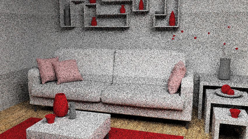
X. Meng et al. / Real-time MC Denoising with the Neural Bilateral Grid

Bilateral Grid. Bilateral filtering [TM98] is a renowned nonlinear                       for frame i as
image processing technique for its advantages in smoothing im-
ages while preserving edges. Paris and Durand [PD06] reformulate                                     Mi (p) = Φ {ri |gi } (p) = ∑ ri ( j)δ(gi ( j) − p),                 (1)
                                                                                                                                           j
bilateral filtering as fast linear filtering by lifting image data to a
higher dimensional space. Chen et al. [CPD07] formally define the                        where p ∈ R3 is a spatial location, δ is a Dirac impulse, and
bilateral grid and present the edge-aware benefits of bilateral grids                    gi ( j) ∈ R3 is a guide which indicates the desirable placement of
in typical image manipulation tasks. In the bilateral space, Chen                        noisy radiance data of each pixel in the bilateral grid.
et al. [CAWH16] fit affine models to approximate image process-
ing operators and achieve efficient image manipulation for high-                           Then, we apply a three-dimensional filter F to Mi to achieve a
resolution images. The bilateral grid has been generalized to solve                      specific image processing task, that is, noise removal from Monte
colorization and semantic segmentation problems [BP16].                                  Carlo renderings in our application. Our filtering process is a simple
                                                                                         convolution of the filter F with Mi ,
   In addition, Gharbi et al. [GCB∗ 17] train a neural network to
learn affine color transforms to conduct image enhancement. They                                      Mi′ (p) = Mi ⊛ F (p) = ∑ F (gi ( j) − p)ri ( j),                   (2)
                                                                                                                                       j
embed the low-resolution input as coefficients in the bilateral space
and use the sliced coefficients to perform a pointwise transforma-                       where ⊛ is a three dimensional convolution. This equation can be
tion. Motivated by the edge-aware advantage of the bilateral grid,                       interpreted as splatting each noisy pixel ri ( j) into the grid using a
we incorporate the neural bilateral grid in our denoising pipeline.                      filter kernel F (gi ( j) − p) that is centered at the position gi ( j) given
Different from Gharbi et al. [GCB∗ 17], we embed the noisy radi-                         by the guide.
ance data in the bilateral grid by accumulating multiple neighboring
                                                                                            For the next step, we reconstruct frame i by extracting data from
pixels into a specific grid element, and slice directly from the grid
                                                                                         the processed bilateral grid Mi′ . This operation is called slicing,
to get the denoised data. Our approach avoids the explicit computa-
tion of per-pixel weights for large kernels and achieves high-quality                                                  Ri ( j) = Mi′ (gi ( j)),                          (3)
denoising with fast, spatially uniform filters.
                                                                                         where Ri is the reconstructed image, Ri ( j) is its j-th pixel, and
                                                                                         slicing is performed by reading the grid at the 3D location gi ( j)
                                                                                         using the same guide as for grid construction.
3. Problem statement                                                                       By chaining the above three operations together, we define the
                                                                                         denoising process as a unified operation
Our goal is to learn a denoiser to reconstruct noise-free images
from noisy rendering data. With existing full-fledged renderers and                                           Ri ( j) = {Φ {ri |gi } ⊛ F } (gi ( j))                     (4)
typical scene description data, we can generate a large number of
noisy images rendered with k samples-per-pixel (k spp) and their                         which suggests an end-to-end denoising process from input noisy
approximate noise-free versions (4096 spp). In addition to noisy                         radiance to denoised results.
images, auxiliary features like normal, depth, and albedo can read-                         A key idea in our approach is that for a suitable guide gi we can
ily be obtained as by-products from the rendering process. We gen-                       use a very simple and fast convolution operation F. Hence, instead
erate a set of paired data of N frames {((r1 , f1 ),t1 ), ((r2 , f2 ),t2 ),              of manually crafting a guide, we propose to use a neural network
. . ., ((rN , fN ),tN )}, where ri , fi stands for noisy radiance and aux-               C to predict a guide. In addition to noisy radiance ri , we also feed
iliary features of frame i, and ti is the noise-free ground truth of                     available auxiliary features fi to the neural network. This process
frame i. Given the dataset, we formulate the denoising problem as                        can be expressed as
a supervised learning task. In this paper, we propose a novel ar-
chitecture which composites a neural network and neural bilateral                                               gi ( j) = ( jx , jy , CΘ (ri , fi )( j)),                (5)
grids to solve the problem.
                                                                                         where Θ represents trainable parameters of our neural network.
   The traditional bilateral grid is designed as a three-dimensional                     Note that for simplicity, the pixel coordinates jx , jy are re-used
data structure [CPD07], although generalizations to higher dimen-                        as the first two coordinates of the guide, and the neural network
sional structures are possible. To process an image with a bilateral                     only predicts the third coordinate. Hence the neural network output
grid, the image is firstly mapped to the 3D bilateral grid, then the                     CΘ (ri , fi ) is an effective 2D guide image.
bilateral grid is processed according to the specific image process-
                                                                                            By substituting the above form of gi into Equation 4, we can
ing task, and finally the output is obtained by extracting a 2D slice
                                                                                         further rewrite the denoising operation as
of the 3D grid.
                                                                                                 Ri ( j) = {Φ {ri |CΘ (ri , fi )} ⊛ F} ( jx , jy , CΘ (ri , fi )( j)).   (6)
   In a similar spirit, we design a neural bilateral grid for denoising
Monte Carlo renderings. A bilateral grid Mi is a three dimensional                       Intuitively, we drive the neural network to learn to place noisy radi-
embedding of an image, which we can write as Mi : R3 → R3 ,                              ance data in a bilateral grid in an optimal way. The neural network
where the input is a location in 3D space, and the output is a ra-                       is trained in an end-to-end manner based on the training data. We
diance value. First, we set up a bilateral grid by embedding noisy                       define a loss function L to measure the difference between one de-
radiance data into the grid. Let us denote the j-th pixel in a noisy                     noised image Ri and its ground truth image ti . To obtain the opti-
input frame as ri ( j). We denote the construction of a bilateral grid                   mal parameters Θopt of the neural network, we minimize the loss

 c 2020 The Author(s)
Eurographics Proceedings c 2020 The Eurographics Association.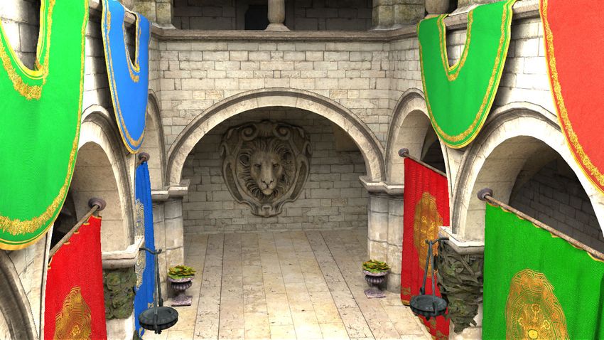
X. Meng et al. / Real-time MC Denoising with the Neural Bilateral Grid

function with modern gradient descent algorithm, given a set of k               three sampling rates ηh , ηw and ηd for the three axes of the grid.
training samples,                                                               The resolution of a bilateral grid is related to the sampling rates by
                                      K

                                                                                                                  h      w       d
                   Θopt = arg minΘ ∑ L(Ri ,ti ).                     (7)                       (H,W, D) = ⌈ ⌉, ⌈ ⌉, ⌈ ⌉ ,                          (8)
                                      i=1
                                                                                                                 ηh      ηw     ηd
                                                                                where h and w are the height and width of the two-dimensional
                                                                                noisy image, and d is the range of the guide, which we set to 255.
4. Neural Bilateral Grid Denoiser                                                   We then directly obtain a filtered, discrete grid by computing the
In this section, we introduce the overall multi-scale architecture of           filtered grid Mi′ as in Equation 2 and evaluating it at the discrete
our neural bilateral grid denoiser. As shown in Figure 1, the input             grid points. For simplicity, we use a tent filter
data consist of path-traced noisy radiance and its auxiliary features.
                                                                                  T (x, y, z) = max (1 − |x|, 0) · max (1 − |y|, 0) · max (1 − |z|, 0) (9)
Input data are sent to a GuideNet to predict guide images (Sec-
tion 4.1). Following that, guide images instruct the construction of            to splat the noisy data into the grid, that is F = T in Equation 2.
the bilateral grid (Section 4.2). In the next stage, we reuse guide im-         The definition of T assumes unit spacing between grid cells. To
ages to slice data from the bilateral grid and reconstruct a denoised           avoid the singularity in the derivative of the absolute value function
                                                                                                               √
image (Section 4.3). Lastly, we describe how to train the GuideNet              | · |, we replace |a| in T with a2 + ε, where a can be x, y or z and
in an end-to-end fashion based on the complete pipeline including               ε is a small number 1e − 7. The function T now provides non-zero
grid construction and slicing (Section 4.4).                                    gradients for points within its support, which is what we desire.
   In addition, we design a multi-scale architecture (Section 4.5)                  Grid cells in a bilateral grid Mi′ are initialized with zero. Given
with three bilateral grids of different resolutions. At each scale, the         the tent function as the splatting filter, the noisy value ri ( j) of pixel
same construction and slicing on a bilateral grid are executed in-               j can be added to the grid cell simply by an equivalent tri-linear
dependently. The final output is a weighted combination of results              interpolation. Following Equation 2, for a grid point p with coordi-
from multiple scales. Finally, we include temporal enhancement                  nates p = (x, y, z), its stored value is
operations (Section 4.6) to ensure temporal stability when denois-
ing image sequences.                                                                                                 ∑ j w p, j · ri ( j)
                                                                                                        Mi′ (p) =                         ,                     (10)
                                                                                                                         ∑ j w p, j

4.1. Guide Prediction                                                           where the sum is over all pixels j of the noisy image Ri . The nor-
                                                                                malization by the sum of the weights ∑ j w p, j is necessary because
We design the GuideNet module in Figure 1 with a convolutional                  of the nonuniform distribution of splatting kernels in the bilateral
neural network (CNN) architecture. For denoising 1-spp input at                 grid. The weights w p, j for each pair of grid point p and pixel j are
real-time speed, we use a two-layer CNN (Figure 2, left). For
denosing 64-spp input that are not produced in real-time, we uti-                                 w p=(x,y,z), j=(m,n) = T (gi ( j) − p) ,                      (11)
lize a seven-layer CNN architecture that contains a five-layer dense
block (Figure 2, right). For each layer in the block, we concatenate            where for a pixel j = (m, n) on the noisy frame i, its position in the
their feature maps to its following layers. In both architectures, we           bilateral grid is given by the guide gi ( j) as
set the 2D size of convolution as 5 × 5. We employ rectified linear                            gi ( j) = (m/ηh , n/ηw , CΘ (ri , fi )( j)/ηd ).                 (12)
(ReLU) [NH10] activations for layers before the last one, while we
use Sigmoid activation for the last layer.                                      In practice, pixels whose weights w p, j are guaranteed to be zero
                                                                                can be excluded from Equation 10.
Data decomposition. As a preprocessing step, we factor out
albedo from the noisy radiance data. Symmetrically, we multiply
the albedo back to the denoised radiance data at the end. By re-                4.3. Bilateral Grid Slicing
moving albedo, the neural network can focus on learning to predict
a guide based on noise patterns in smooth irradiance data. The de-              We reconstruct a denoised image by slicing the bilateral grid. This
composition and composition of albedo requires only one division                is a semantically symmetrical procedure to the bilateral grid con-
and one multiplication, incurring negligible computational costs.               struction. With a guide gi , reconstructing a pixel j involves evalu-
                                                                                ating Mi′ (gi ( j)) as formulated in Equation 3.
                                                                                   Since our grid Mi′ is discrete, this requires continuous interpola-
4.2. Bilateral Grid Construction
                                                                                tion of the grid values. Similar as for splatting noisy data into the
The bilateral grid in our framework is a three-dimensional grid with            grid described by Equation 10, we employ tri-linear interpolation
a resolution H × W × D (Figure 1). To splat a pixel with RGB                    using the tent filter T to interpolate values from the bilateral grid.
color channels onto the grid, we leverage the corresponding scalar
                                                                                   To compute a pixel j in the sliced image Ri ( j), we return a
value in the guide image to instruct the placement of the three-
                                                                                weighted combination of grid values based on the interpolation fil-
dimensional spectrum vector as a whole.
                                                                                ter. By splatting a 2D noisy image to a 3D bilateral grid, the bilat-
  To map a two-dimensional image to a bilateral grid, we define                 eral grid is sparsely populated and some of its cells remain empty.

                                                                                                                                                c 2020 The Author(s)
                                                                                                         Eurographics Proceedings c 2020 The Eurographics Association.
X. Meng et al. / Real-time MC Denoising with the Neural Bilateral Grid
w0 guide0
Frame i -1
D
W
Color
w/ o albedo w0
Pre- Grid Grid
temporal grid 0
accum. creation slicing
H
Frame i GuideNet
w1 guide1
Norm. …
depth, normal Color
albedo w/ o albedo
w1
Grid Grid Weighted
creation grid 1 slicing composition
Color w2 guide2
w/ o albedo
Frame i
w2 output
Grid Grid
creation grid 2 slicing
Albedo
Figure 1: Overview of our temporal, multi-scale neural bilateral grid denoiser. The temporally accumulated noisy radiance without albedo,
and auxiliary features including depth, normals, and albedo of each frame are sent to a GuideNet. GuideNet is trained in an end-to-end
fashion to embed the noisy image data in the bilateral grid, and to slice radiance from the bilateral grid. In addition, we apply a multi-
resolution approach using grids at three resolutions, and GuideNet also provides blending weights to combine their outputs. Finally, we
multiply the albedo back to form a denoised frame.
GuideNet-1 GuideNet
GuideNet-2
Also, we could set up another neural network to produce such a
guide gΘ′ . We, however, do not observe significant improvement
Conv Conv Conv Conv of denoising performance by computing two independent guides.
… Hence, we employ only one neural network and reuse the predicted
guide for both construction and slicing of a bilateral grid.
20 5 20 10 10 5
5 Convs Post-processing. The denoised images from the slicing step are
irradiance data without albedo. As a post-processing, we multiply
Figure 2: Architectures of GuideNet. For 1-spp input, a two-layer the albedo data in the auxiliary features back to the denoised result
CNN architecture (left) is used. For 64-spp input, a seven-layer ar- Ri , and obtain an output R̃i = Ri ∗ falbedo .
chitecture (right) with a dense block is employed. The dense block
contains five layers and the purple dots are concatenations. The 4.4. End-to-end Training
number of filters of each layer are shown below each layer. The
output consists of three guide images and two pixel-wise weights. We train our GuideNet that we use to predict the guide to mini-
mize the objective as formulated in Equation 7. We use the L1 loss
function, which computes the mean absolute difference between
denoised results and ground truth images, since it correlates well
That is, these cells did not receive any contributions during splat- with the difference perceived by humans. Hence, our loss is
ting. We skip empty grid cells with zero values and include a renor- 1 K
∑ (14)
malization, L= S R̃i − S (ti ) .
K i=1
∑{p|Mi′ (p)6=0} Mi′ (p) · w p, j
Ri ( j) = , (13) Here, ti represents a ground truth image. S represents an image
∑{p|Mi′ (p)6=0} w p, j processing function associated with the training dataset (details are
in Section 5). The input noisy radiance data are processed by S
where {p|Mi′ (p) 6= 0} indicates the set of integer grid points where
before entering the neural network. Note that we use high dynamic
the grid is non-zero. The weights w p, j are computed identically to
range data in the bilateral grid construction and slicing modules to
the splatting weights in Equation 11, using the same tent filter T
preserve information of the original dynamic range.
and guide gi ( j). In practice, the summation in Equation 13 can be
limited to grid cells within the support of the interpolation filter In our pipeline, bilateral grid construction and bilateral grid slic-
centered at gi ( j). Note that in general the splatting filter does not ing modules are inserted between the neural network and the final
need to be the same as the interpolation filter for slicing. In addition, output. To allow error back-propagation from the final output to the
we could also use two different guides for splatting and slicing. In neural network, we derive analytical gradients of the two modules.
our experiments, however, we did not observe any benefits of this. Specifically, the gradient of bilateral grid with respect to the guide
c 2020 The Author(s)
Eurographics Proceedings c 2020 The Eurographics Association.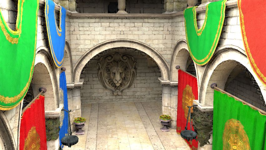
X. Meng et al. / Real-time MC Denoising with the Neural Bilateral Grid

∂M
∂g
    is computed for constructing the bilateral grid M. For the slicing
module, we compute gradients of the denoised output with respect
                            ∂R
to the grid and the guide, ∂M   and ∂R
                                     ∂g
                                        . For details of the analytical
derivatives, we refer readers to our supplementary material.

4.5. Multi-scale Bilateral Grids
Given the input noisy frame, we build a 3-scale pyramid of bilateral
grids as shown in Figure 1. We denote the scales using index s ∈
{0, 1, 2}. As in Section 4.2, the resolution of a grid of scale s is
given by sampling rates (ηsh , ηsw , ηsd ). The bilateral grid at scale 0
has the original, highest resolution (η0h , η0w , η0d ) = (ηh , ηw , ηd ). For    Figure 3: An overview of reference frames of scenes included in
lower scales, we use (ηs+1     s+1 s+1                s    s     s
                        h , ηw , ηd ) = (2ηh , 2ηw , 2ηd ). That is,              our own dataset.
the following scale will halve the resolution of the previous scale
along every direction of the grid.
   For each scale s, we generate a separate guide image from the                  challenges for modern renderers. See Figure 3 for an overview of
GuideNet, and use it to instruct the construction of the bilateral grid           scenes used in our dataset. For every scene, we rendered a consec-
with the appropriate resolution. Similarly, we slice each bilateral               utive sequence of 100 frames. For each frame, we use the built-in
grid scale with its individual guide image and obtain reconstructed               path tracer of Tungsten with its default settings to render 1 and
radiance Rsi independently. To form the final radiance, we compute                64-spp noisy images. The corresponding ground truth images are
the weighted composition                                                          rendered with 4096 spp.
                    Ri = w0 · R0i + w1 · R1i + w2 · R2i ,                (15)        From the noisy images, we noticed visible outlier pixels whose
where w0 , w1 , w2 are pixel-wise weight maps. We reuse the                       values are significantly higher than their neighbors. Splatting out-
GuideNet to predict weight maps 0 ≤ w0 ≤ 1, 0 ≤ w1 ≤ 1 and set                    liers with extremely high value to the bilateral grid will cause arti-
w2 = 1 − (w0 + w1 ) to normalize the weights.                                     facts since these values cannot be effectively spread. To reduce the
                                                                                  impact of outliers, we apply a preprocessing step [KBS15] to detect
                                                                                  and suppress outlier pixels.
4.6. Temporal Enhancement
                                                                                     The GuideNet accepts images with low dynamic range, so we
When denoising consecutive frames of a video, temporal sta-                       use the function S (Equation 14) to convert input noisy radiance
bility is important for perceived visual quality because the ran-                 data to low dynamic range data. S represents the gamma correc-
dom residual, low frequency noise patterns vary from frame to                     tion function for BMFR dataset with exponent of 1/2.2, whereas
frame. To improve temporal stability, we utilize a pre-stage of                   for the Tungsten dataset it represents the Tungsten tone mapping
temporal enhancement to accumulate consecutive 1-spp noisy ra-                    operator [Bit16].
diance data without albedo (Figure 1) by the reprojection tech-
nique [KIM∗ 19, SKW∗ 17], where we set the decay factor of the                    Training and Testing. For both datasets we hold out frames of
previous frame to 0.2.                                                            one scene as test data, and use the remaining images of the other
                                                                                  scenes as the training data. In addition, we randomly select frames
                                                                                  of one scene from the training data to function as validation data.
5. Experimental Setup
                                                                                  This means we use a separate network to obtain test results for
Datasets Preparation. We used two datasets in our experiments.                    each scene, where the network is trained using data only from the
We firstly adopt an existing dataset from the work of Koskela                     other scenes. Hence the performance on test data can serve as an
et al. [KIM∗ 19], which we call the BMFR dataset. The dataset                     indication of the generalization ability of the trained denoiser.
is comprised of a set of 360 noisy 1-spp rendering images and
                                                                                     During both the training and the inference stage, inputs to the
their ground truth images from six scenes: Classroom, Living-room,
                                                                                  GuideNet are comprised of low dynamic range (LDR) radiance
San-miguel, Sponza, Sponza-glossy, Sponza-moving-light. These
                                                                                  with albedo (3 channels) and auxiliary features (7 channels), which
scenes are configured with diverse materials, illumination and cam-
                                                                                  include 3-channel albedo, 3-channel normal and 1-channel depth.
era movements. Each scene has 60 consecutive frames and their
                                                                                  The input to the bilateral grid is the high dynamic range (HDR)
ground truth images are rendered with more than 2048 spp to ob-
                                                                                  radiance without albedo. Both the radiance and auxiliary features
tain approximate noise-free appearance. The image resolution is
                                                                                  are normalized to the range between 0 and 1 before sending to the
1280 × 720.
                                                                                  network. In the training stage, we use image patches at a resolution
   In addition, we build a new dataset of publicly available Tung-                of 128 × 128. We randomly sample 60 such crops from each frame
sten scenes [Bit16] using the Tungsten renderer and we call it Tung-              of training data to form a training dataset, and sample 20 crops to
sten dataset. Our dataset includes rendered images at a resolution of             build a validation dataset. In the inference stage, the inputs to the
1280 × 720 from nine scenes, which cover a wide variety of geom-                  network consist of the full resolution (1280 × 720) frames from the
etry scales, material types, and lighting effects that reflect typical            test data.

                                                                                                                                                 c 2020 The Author(s)
                                                                                                          Eurographics Proceedings c 2020 The Eurographics Association.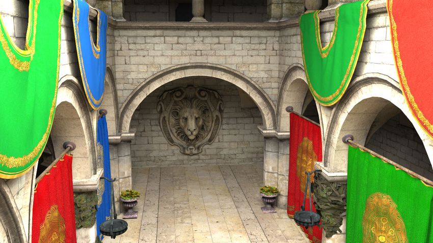
X. Meng et al. / Real-time MC Denoising with the Neural Bilateral Grid

Implementation. Our denoiser is implemented in Tensor-                                   our approach. Note also in NFOR, the albedo processing is not ap-
Flow [AAB∗ 15]. The bilateral grid construction and slicing mod-                         plied. To evaluate denoising performance quantitatively, we adopt
ules have been implemented in CUDA as plug-in operators to inte-                         standard metrics including PSNR and SSIM [WSB03] (see also er-
grate with TensorFlow. Before training, weights of the neural net-                       ror maps in the supplementary material).
work are initialized with uniform random value ranges from -1 to 1.
Three sampling rates for the bilateral grid at scale-0 are configured                               30                                        Ours (3-grid)
                                                                                                                          Ours (1-grid)
as ηh = ηw = 4, ηd = 4. Depending on the GPU memory size, we                                        28
                                                                                                                                                                   MR-KP (5-layer)
                                                                                                                                                                                        NFOR
use mini-batches of size 20 in training. Because the full frames for                                26
                                                                                                            BMFR                                  MR-KP (1-layer)

                                                                                             PSNR
testing are larger than the crops for training, we set the mini-batch                                                                                              ONND
                                                                                                    24
size to 10 for testing. We train the pipeline in an end-to-end fashion                                                       SVGF
using Adam [KB14]. We set the learning rates to 0.0001 and keep                                     22

the default values for the other parameters. A typical training time                                20
for one test scene using 100 epochs on an Nvidia RTX 2080 GPU                                           1         2            4          8       16          32     64     128       256
                                                                                                    0.94
is about 14 hours.                                                                                                          Ours (1-grid)                           MR-KP (5-layer)
                                                                                                    0.92                                      Ours (3-grid)                             NFOR
                                                                                                                BMFR           SVGF
                                                                                                    0.90

                                                                                             SSIM
6. Results and Discussion                                                                                                                         MR-KP (1-layer)
                                                                                                    0.88
We evaluate our approach by comparing it with state-of-the-art                                      0.86
                                                                                                                                                                   ONND

methods in terms of both image quality and running speed.
                                                                                                    0.84
                                                                                                            1         2         8  4   16       32     64   128      256
                                                                                                                                 Timing (ms)
6.1. Evaluation Methods and Error Metrics                                                                Measured with RTX 2080            Measured with Nvidia Titan X
                                                                                                                     Measured with Intel Core i7-8700 CPU
Since our approach aims at real-time denoising, we mainly fo-
cus our comparisons on existing real-time denoising approaches.                          Figure 4: Scatter plots of PSNR-timing and SSIM-timing of all
Specifically, we report results from the recent BMFR ap-                                 evaluated denoisers.
proach [KIM∗ 19], the OptiX Neural Network Denoiser (ONND)
which is adapted from [CKS∗ 17] and is available in the
OptiX 5.1 engine, Spatio-temporal Variance-Guided Filtering                              6.2. Quality Comparisons
(SVGF) [SKW∗ 17], and a Multi-Resolution variant of Kernel Pre-
diction CNN (MR-KP) denoiser [BVM∗ 17]. In addition, we also                             Our key objective is to achieve very fast denoising for low quality
include a comparison with an off-line denoiser, NFOR [BRM∗ 16].                          data such as 1-spp path tracing. In this scenario, we use a light-
For BMFR, SVGF and NFOR, we use implementations provided                                 weight 2-layer convolutional neural network as the GuideNet and
by their authors.                                                                        three relatively coarser bilateral grids to strike the balance between
                                                                                         fast speed and good quality. We demonstrate that our approach can
   The original kernel prediction denoiser [BVM∗ 17] is designed                         outperform the previous state of the art in this scenario.
for off-line denoising and requires several seconds to process a sin-
                                                                                            Owing to the scalable and modular architecture of our denoiser,
gle 720p frame. Similar to our multi-scale design, we have adapted
                                                                                         we can tailor the architecture of the GuideNet and adjust the res-
the multi-resolution variant (MR-KP) [VRM∗ 18], which decreases
                                                                                         olution of bilateral grids to adapt to different applications. For 64-
the run time of a basic kernel prediction architecture to the order of
                                                                                         spp data, which are naturally produced with offline settings, we
tens of milliseconds. Hence it is an important comparison point for
                                                                                         have employed a more complex GuideNet, which is designed as
real-time denoising. Details of the architecture of MR-KP can be
                                                                                         a 7-layer DenseNet [HLVDMW17]. We demonstrate competitive
found in the supplementary material. For fair comparison, our MR-
                                                                                         performance in this setting, although denoising data from off-line
KP is trained with the same loss and the same split of dataset as our
                                                                                         rendering is not intended as the main application of our approach.
approach. Also, we perform the same temporal filtering as in our
approach, instead of including it in the kernel prediction denoiser                         For 1-spp input data to our denoiser, we apply pre-stage temporal
itself.                                                                                  accumulation to increase the effective sample count of each frame
                                                                                         as described in Section 4.6. To ensure fairness, we use the same
   ONND is provided as a black box module in OptiX 5.1. It
                                                                                         temporal accumulation for all compared approaches. Our denoiser
is derived from the autoencoder-based denoiser by Chaitanya et
                                                                                         is applicable to reconstruct both single noisy images and a sequence
al. [CKS∗ 17], but ONND differs from the original paper in several
                                                                                         of noisy animated frames. In the following sections, we show de-
aspects: 1) ONND consumes a different set of auxiliary features. 2)
                                                                                         noised results of single frames. Besides, we upload a test suite with
It expects low dynamic range input which has been processed by
                                                                                         an interactive viewer along with this paper to allow readers to view
tone mapping and gamma correction and it outputs low dynamic
                                                                                         and compare all denoised frames.
range data.
   Since ONND operates albedo demodulation and re-modulation                             BMFR dataset. Firstly, we show how our denoiser performs on
in its black box, we send original noisy radiance to it and skip the                     the BMFR dataset. As described in Section 5, we use frames of five
re-modulation of albedo. For BMFR, SVGF and MR-KP, we apply                              scenes as the training dataset, and test the denoiser on frames of the
the same albedo demodulation and re-modulation processes as in                           remaining one scene. Figure 5 shows the comparison of the 51-th

 c 2020 The Author(s)
Eurographics Proceedings c 2020 The Eurographics Association.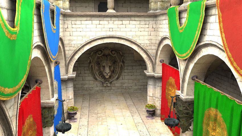
X. Meng et al. / Real-time MC Denoising with the Neural Bilateral Grid

frames of the selected test scene. Our method performs better at             (Figure 2, right) for denoising 64-spp input data. We measure the
preserving regions with highlights, as shown in the closeup on the           average time cost by denoising all frames of the Dining Room scene
lion relief of the Sponza (glossy) scene. The error measurements             of our Tungsten dataset. The average timing for denoising one 720p
are presented in Table 1 and Table 2. It can be observed that our            frame is shown in the third data row of Table 3.
method generally provides low numerical errors. Also, scatter plots
                                                                               Our denoiser in this case runs at 11.7 FPS. Since 64-spp render-
in Figure 4 clearly show that our denoiser performs the best in terms
                                                                             ings execute in offline applications, our denoiser can be applied as
of PSNR and SSIM, meanwhile our denoiser stands a comparable
                                                                             an efficient post-processing process to improve quality of rendered
position for speed.
                                                                             images.
   To measure the time cost of denoising, we apply all denoisers
on the same test data. The mean time cost to denoise a frame is
                                                                             6.3. Ablation Studies
averaged over all test frames. The average timings of all methods
are presented in Table 3. For denoising the BMFR dataset, our de-            Guide Prediction. To analyze the impact of training a neural net-
noiser using a 2-layer GuideNet and a 3-scale bilateral grids (2nd           work to obtain optimized guide images, we compare our approach
row of Table 3) can run at a real-time performance which reaches             to a baseline where the guide image is simply the arithmetic mean
61 frames per second (FPS). Our method does not show obvious                 of the auxiliary features. Figure 7 compares our optimized guide
superiority in denoising quality compared with 5-layer MR-KP, but            images and the baseline on the Sponza scene. The baseline shows
ours (16.460 ms) is faster than the 5-layer MR-KP (39.537 ms). If            apparent artifacts around edges because it cannot guide a correct
we reduce the capacity of MR-KP to make it faster by going to one            splatting of noisy radiance. On the contrary, our approach learns
layer, it still ends up with slower speed and lower denoising quality        optimal guide images to place noisy radiance in the grid and gives
compared to ours.                                                            better reconstructed results.
                                                                                We further visualize the three guide images of three scales and
Tungsten dataset. For our Tungsten dataset, we rendered noisy
                                                                             the single guide image of the baseline in Figure 8. As shown in
image sequences at 64-spp. Figure 6 shows the comparisons of de-
                                                                             the closeups, our guides successfully distinguish the smooth dim
noised results of test scenes extracted from our dataset. Our test
                                                                             region from the sharp edge of a rod, while the baseline is affected
scenes contain a wide range of challenges for existing rendering
                                                                             by multiple features and leads to artifacts in its output.
techniques, including difficult glossy and specular light transport
and complex visibility issues. Although rendered with 4096 spp,
                                                                             Multi-scale bilateral grids. Our denoiser uses a three-scale hi-
the reference images still show some residual noise as in the Living
                                                                             erarchy of bilateral grids. The final result is reconstructed by a
Room scene and the Dining Room scene. In our experiments, input
                                                                             weighted blending of denoised images from the three scales. Based
data with and without removing outliers are tested. Experiments
                                                                             on the experiments on the test scenes presented in Figure 5, we cal-
show that outlier removal leads to more visually pleasing results,
                                                                             culate the average PSNR for denoised images at each scale. Then,
thus we adopt these results in the following comparisons.
                                                                             we compare the arithmetic mean of three PSNRs with the PSNR of
  As shown in the Living Room scene (row 1 of Figure 6), our                 the final result produced by our weighted blending. As summarized
approach excels at preserving edges of the lights on the ceiling and         in Table 5, the weighted multi-scale approach consistently produces
edges of thin tree branches with slender structure, while NFOR and           higher quality than any of the individual scales.
BMFR slightly blur the edges. Due to the blockwise reconstruction
                                                                                The supplementary document includes additional ablation stud-
manner, BMFR will remove geometry details in some local regions.
                                                                             ies to compare different architectures of our denoiser.
   Also, our denoiser can robustly reconstruct the shadow cast by
the shutter blinds in the Dining Room scene (row 2 of Figure 6),
                                                                             6.4. Limitations
whereas BMFR misses the regular structure of shadow. NFOR,
which utilizes more sophisticated auxiliary features, can recon-             Specular light transport. Specular light paths are notoriously dif-
struct the shadow with the highest quality, but it also leads to a           ficult to sample, thus often leading to extreme noise. In this sce-
much slower speed. The blue insets of the Dining Room scene show             nario, features such as albedo textures also provide little useful
surfaces with glossy materials and highlights. Our denoiser, ONND            information to the denoiser. The blue insets of the Living Room
and MR-KP effectively removes the noise and preserves the high-              scene in Figure 6 shows such a case, where all of the denoisers fail
light regions, whereas BMFR cannot recover highlight and glossy              at reconstructing the glass vase. Accurately denoising such difficult
reflections. While NFOR shows the highest quality of shadow, it              scenarios remains a challenge for real-time denoisers.
slightly blurs the regions with specular highlights.
                                                                             Generalization to unseen effects. Our scalable neural bilateral
   Table 4 presents the average errors over 100 frames on five
                                                                             grid denoiser is able to provide better visual quality and lower resid-
scenes of our Tungsten dataset. Note that our method with out-
                                                                             ual error on the 1-spp BMFR dataset and competitive performance
lier removal leads to a slight drop of PSNR and SSIM. To avoid
                                                                             on the 64 spp Tungsten dataset, but it has several generalization is-
affecting error metrics of other denoisers, we do not apply outlier
                                                                             sues. Since none of the datasets include scenes with depth of field,
removal to them. In our experiment, we exploit the outlier removal
                                                                             motion blur, or volumetric media, our denoiser may yield poor per-
step because it can quench outliers and achieve visually better re-
                                                                             formance or give artifacts on such scenes with unseen effects. This
sults.
                                                                             problem can currently only be mitigated by increasing the general-
  As stated before, we use a GuideNet with a 7-layer architecture            ity of training scenes.

                                                                                                                                            c 2020 The Author(s)
                                                                                                     Eurographics Proceedings c 2020 The Eurographics Association.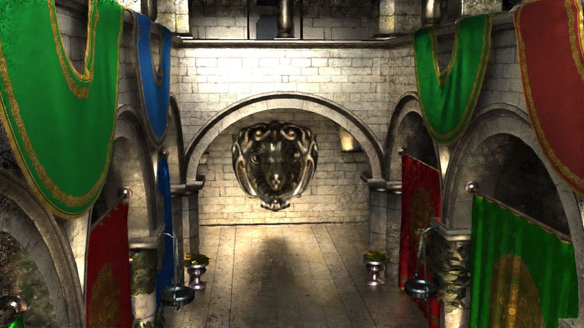
X. Meng et al. / Real-time MC Denoising with the Neural Bilateral Grid

                              Ours                                   1 spp        NFOR           BMFR          ONND            MR-KP     Ours      Reference
Living room
Sponza moving light
Sponza glossy
Classroom
San Miguel

   Figure 5: Comparisons on the 1-spp BMFR dataset showing the 51-th frame from the animated sequence. Each row represents an independent
   experiment where the displayed scene is for test and other scenes are used for training. References are rendered with 4096 spp. For each
   scene, closeups of the orange square are shown on the top row and closeups of the blue square are on the bottom row.

   7. Conclusions                                                                           tract denoised radiance. The proposed neural bilateral grid denoiser
                                                                                            is scalable and it allows us to tailor the design of each module ac-
   We have introduced a novel and practical neural bilateral grid de-                       cording to real-time or offline applications. Our experiments have
   noiser, that can reconstruct extremely noisy rendering images in                         demonstrated that, with a two-layer shallow GuideNet, it is able to
   real-time. At the core of our approach, we utilize an efficient neu-                     deliver better denoised results in terms of both visual quality and
   ral network, GuideNet, to learn to splat noisy radiance data onto a                      numerical error metrics for 1-spp input data. By using a deeper
   hierarchy of multi-scale bilateral grids and then slice the grid to ex-

    c 2020 The Author(s)
   Eurographics Proceedings c 2020 The Eurographics Association.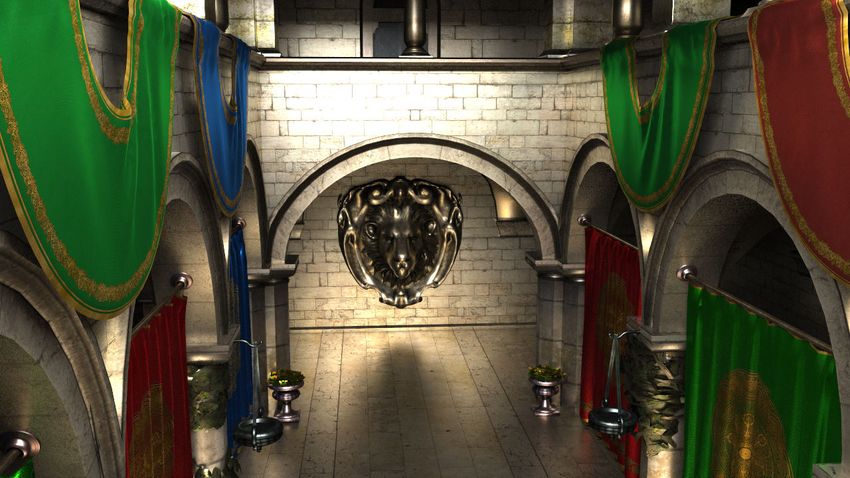
X. Meng et al. / Real-time MC Denoising with the Neural Bilateral Grid

Table 1: A comparison of average PSNR values (higher is better) for evaluating our trained denoisers on 1-spp BMFR test data (see
supplementary document for other error metrics). MR-KP 5-layer represents the 5-layer kernel prediction architecture and MR-KP 1-layer
represents the 1-layer kernel prediction architecture. Ours 3-grid represents the 2-layer, 3-grid architecture and Ours 1-grid stands for the
2-layer, 1-grid architecture. We achieve the highest scores except for PSNR of Classroom and Sponza (mov. light), while taking less than ten
milliseconds (see Table 3).

                                                                                       PSNR
                 Scene
                                   NFOR       BMFR       ONND      SVGF      MR-KP(5-layer)      MR-KP(1-layer)        Ours(3-grid)        Ours(1-grid)
               Classroom           29.872     28.965     27.312    25.034         32.177              31.392               31.519              31.284
              Living room          31.304     30.025     25.586    27.239         31.995              30.311               32.294              28.317
              San Miguel           21.811     20.969     20.172    18.736         22.950              22.482               23.650              23.940
                Sponza             30.377     31.111     24.698    24.401         29.476              29.912               33.188              32.787
            Sponza (glossy)        25.974     25.005     23.460    20.917         26.447              27.303               29.548              29.459
           Sponza (mov. light)     21.999     17.377     22.291    17.260         25.090              23.637               24.818              24.860

Table 2: A comparison of average SSIM values (higher is better) for evaluating our trained denoisers on 1-spp BMFR test data (see
supplementary document for other error metrics). MR-KP 5-layer represents the 5-layer architecture and MR-KP 1-layer represents the
1-layer architecture. Ours 3-grid represents the 2-layer, 3-grid architecture and Ours 1-grid stands for the 2-layer, 1-grid architecture).

                                                                                       SSIM
                  Scene
                                   NFOR       BMFR       ONND      SVGF      MR-KP(5-layer)      MR-KP(1-layer)        Ours(3-grid)        Ours(1-grid)
               Classroom            0.956      0.955      0.924    0.952          0.972               0.959                0.968               0.966
              Living room           0.967      0.965      0.953    0.950          0.965               0.933                0.968               0.948
              San Miguel            0.799      0.789      0.744    0.790          0.808               0.773                0.820               0.834
                Sponza              0.939      0.948      0.852    0.927          0.963               0.955                0.973               0.973
            Sponza (glossy)         0.901      0.907      0.867    0.913          0.927               0.897                0.941               0.943
           Sponza (mov. light)      0.895      0.858      0.811    0.876          0.948               0.896                0.946               0.947

Table 3: Average time cost of each denoising approach. We sepa-                   [BEM11] BAUSZAT P., E ISEMANN M., M AGNOR M.: Guided image
                                                                                    filtering for interactive high-quality global illumination. In Computer
rately record timings on the Classroom scene of two datasets. For                   Graphics Forum (2011), vol. 30, Wiley Online Library, pp. 1361–1368.
the BMFR dataset, the timing is averaged over 60 Frames, while                      2
the timing is averaged over 100 frames for the Tungsten dataset.                  [Bit16] B ITTERLI B.: Rendering resources, 2016.                 https://benedikt-
                                                                                     bitterli.me/resources/. 6
           Method          Timing (ms)                 Device
     Ours 2-layer 1-grid           9.407        Nvidia RTX 2080                   [BP16] BARRON J. T., P OOLE B.: The fast bilateral solver. In European
     Ours 2-layer 3-grid          16.460        Nvidia RTX 2080                     Conference on Computer Vision (2016), Springer, pp. 617–632. 3
     Ours 7-layer 3-grid          84.988        Nvidia RTX 2080                   [BRM∗ 16] B ITTERLI B., ROUSSELLE F., M OON B., I GLESIAS -
           NFOR                  370.000     Intel Core i7-8700 CPU
           BMFR                    1.600        Nvidia RTX 2080                     G UITIÁN J. A., A DLER D., M ITCHELL K., JAROSZ W., N OVÁK J.:
          ONND                    55.000          Nvidia Titan X                    Nonlinearly weighted first-order regression for denoising monte carlo
           SVGF                    4.400          Nvidia Titan X                    renderings. In Computer Graphics Forum (2016), vol. 35, Wiley Online
      MR-KP(5-layer)              39.527        Nvidia RTX 2080                     Library, pp. 107–117. 2, 7
      MR-KP(1-layer)              25.321        Nvidia RTX 2080
                                                                                  [BSS∗ 13] B ELCOUR L., S OLER C., S UBR K., H OLZSCHUCH N., D U -
                                                                                    RAND F.: 5d covariance tracing for efficient defocus and motion blur.
neural network architecture, its denoising ability is on par with or                ACM Transactions on Graphics (TOG) 32, 3 (2013), 31. 2
outperforms state-of-the-art real-time denoising approaches.
                                                                                  [Bur81] B URT P. J.: Fast filter transform for image processing. Computer
                                                                                    graphics and image processing 16, 1 (1981), 20–51. 2
References                                                                        [BVM∗ 17] BAKO S., VOGELS T., M C W ILLIAMS B., M EYER M.,
[AAB∗ 15] A BADI M., AGARWAL A., BARHAM P., B REVDO E.,                             N OVÁK J., H ARVILL A., S EN P., D EROSE T., ROUSSELLE F.: Kernel-
  ET AL .: TensorFlow: Large-scale machine learning on heterogeneous                predicting convolutional networks for denoising monte carlo renderings.
  systems, 2015. Software available from tensorflow.org. URL: https:                ACM Transactions on Graphics (TOG) 36, 4 (2017), 97. 1, 2, 7
  //www.tensorflow.org/. 7                                                        [CAWH16] C HEN J., A DAMS A., WADHWA N., H ASINOFF S. W.: Bi-
[BBS14] B ELCOUR L., BALA K., S OLER C.: A local frequency analysis                 lateral guided upsampling. ACM Transactions on Graphics (TOG) 35, 6
  of light scattering and absorption. ACM Transactions on Graphics (TOG)            (2016), 203. 3
  33, 5 (2014), 163. 2                                                            [CKS∗ 17] C HAITANYA C. R. A., K APLANYAN A. S., S CHIED C.,
[BEJM15] BAUSZAT P., E ISEMANN M., J OHN S., M AGNOR M.:                            S ALVI M., L EFOHN A., N OWROUZEZAHRAI D., A ILA T.: Interactive
  Sample-based manifold filtering for interactive global illumination and           reconstruction of monte carlo image sequences using a recurrent denois-
  depth of field. In Computer Graphics Forum (2015), vol. 34, Wiley On-             ing autoencoder. ACM Transactions on Graphics (TOG) 36, 4 (2017),
  line Library, pp. 265–276. 2                                                      98. 1, 2, 7

                                                                                                                                                 c 2020 The Author(s)
                                                                                                          Eurographics Proceedings c 2020 The Eurographics Association.
X. Meng et al. / Real-time MC Denoising with the Neural Bilateral Grid
Table 4: Error measurements for our trained denoisers on test data of the Tungsten dataset, which is rendered at 64 spp and does not use
temporal accumulation as a pre-process. ’Ours’ denotes our denoiser with outlier removal preprocessing, whereas ’Ours wo’ is without
outlier removal. We use the 7-layer 3-grid architecture.
PSNR SSIM
Scene
NFOR BMFR ONND MR-KP Ours wo Ours NFOR BMFR ONND MR-KP Ours wo Ours
Bedroom 35.0524 25.6327 34.4377 36.7279 35.9827 35.5340 0.9730 0.9235 0.9707 0.9774 0.9736 0.9725
Dining room 36.3385 25.8633 37.9529 36.8787 37.3093 37.0157 0.9798 0.9063 0.9699 0.9812 0.9789 0.9757
Ours 64 spp NFOR BMFR ONND MR-KP Ours Reference
Living Room
Dining room
Figure 6: Visual quality comparisons on the Tungsten dataset rendered at 64spp. We show a single frame from the animated sequences and
do not use temporal accumulation (see additional comparisons on three other test scenes in the supplementary document). We use the 7-layer
3-grid architecture. For each scene, orange insets are shown on the top row and blue insets are on the bottom row.
Table 5: Average PSNR values of images from three grid scales, D URAND F.: Deep bilateral learning for real-time image enhancement.
ACM Transactions on Graphics (TOG) 36, 4 (2017), 118. 1, 3
the arithmetic mean of the three scales, and the final output using
weighted blending. The PSNR of individual scales and the mean [GLA∗ 19] G HARBI M., L I T.-M., A ITTALA M., L EHTINEN J., D U -
RAND F.: Sample-based monte carlo denoising using a kernel-splatting
are consistently lower than the the final output. network. ACM Transactions on Graphics (TOG) 38, 4 (2019), 125. 1, 2
Scene Scale 0 Scale 1 Scale 2 3-scale Mean Final output [HLVDMW17] H UANG G., L IU Z., VAN D ER M AATEN L., W EIN -
BERGER K. Q.: Densely connected convolutional networks. In Proceed-
Living room 29.7854 25.6374 32.2906 29.2378 32.2937
Sponza mov. light 23.5954 24.4703 24.7603 24.2754 24.8176 ings of the IEEE conference on computer vision and pattern recognition
Sponza glossy 25.2993 28.8369 29.4113 27.8492 29.5481 (2017), pp. 4700–4708. 7
Classroom 30.4996 29.3692 31.1660 30.3449 31.5185 [HST10] H E K., S UN J., TANG X.: Guided image filtering. In European
San Miguel 19.0538 22.9720 23.4500 21.8253 23.6504 conference on computer vision (2010), Springer, pp. 1–14. 2
[KB14] K INGMA D. P., BA J.: Adam: A method for stochastic optimiza-
tion. arXiv preprint arXiv:1412.6980 (2014). 7
[KBS15] K ALANTARI N. K., BAKO S., S EN P.: A machine learning ap-
[CPD07] C HEN J., PARIS S., D URAND F.: Real-time edge-aware image proach for filtering monte carlo noise. ACM Trans. Graph. 34, 4 (2015),
processing with the bilateral grid. In ACM Transactions on Graphics 122–1. 2, 6
(TOG) (2007), vol. 26, ACM, p. 103. 3
[KHL19] K ETTUNEN M., H ÄRKÖNEN E., L EHTINEN J.: Deep convolu-
[DSHL10] DAMMERTZ H., S EWTZ D., H ANIKA J., L ENSCH H.: Edge- tional reconstruction for gradient-domain rendering. ACM Transactions
avoiding à-trous wavelet transform for fast global illumination filtering. on Graphics (TOG) 38, 4 (2019), 126. 2
In Proceedings of the Conference on High Performance Graphics (2010),
Eurographics Association, pp. 67–75. 2 [KIM∗ 19] KOSKELA M., I MMONEN K., M ÄKITALO M., F OI A., V I -
ITANEN T., JÄÄSKELÄINEN P., K ULTALA H., TAKALA J.: Blockwise
[ETH∗ 09] E GAN K., T SENG Y.-T., H OLZSCHUCH N., D URAND F., multi-order feature regression for real-time path-tracing reconstruction.
R AMAMOORTHI R.: Frequency analysis and sheared reconstruction for ACM Transactions on Graphics (TOG) 38, 5 (2019), 138. 2, 6, 7
rendering motion blur. In ACM Transactions on Graphics (TOG) (2009),
[KKR18] K UZNETSOV A., K ALANTARI N. K., R AMAMOORTHI R.:
vol. 28, ACM, p. 93. 2
Deep adaptive sampling for low sample count rendering. In Computer
[GCB∗ 17] G HARBI M., C HEN J., BARRON J. T., H ASINOFF S. W., Graphics Forum (2018), vol. 37, Wiley Online Library, pp. 35–44. 2
c 2020 The Author(s)
Eurographics Proceedings c 2020 The Eurographics Association.X. Meng et al. / Real-time MC Denoising with the Neural Bilateral Grid
Ours Input Baseline Ours Reference
PSNR 10.8283 28.0615 31.7794
SSIM 0.1965 0.9506 0.9692
Figure 7: Comparisons between our method and a baseline that computes guide images by simply averaging all auxiliary features. The test
data is a 1-spp rendered image from the Sponza scene.
Baseline guide Level 0 Level 1 Level 2
Figure 8: We visualize a baseline approach using the arithmetic mean of the auxiliary feature channels as guide image, and our three
optimized guide images of the three grid scales produced by the trained GuideNet. As shown in the closeups, our guides effectively instruct
the correct placement of radiance around edges.
[KMA∗ 15] K ETTUNEN M., M ANZI M., A ITTALA M., L EHTINEN J., [RMZ13] ROUSSELLE F., M ANZI M., Z WICKER M.: Robust denois-
D URAND F., Z WICKER M.: Gradient-domain path tracing. ACM Trans- ing using feature and color information. In Computer Graphics Forum
actions on Graphics (TOG) 34, 4 (2015), 123. 2 (2013), vol. 32, Wiley Online Library, pp. 121–130. 2
[KS13] K ALANTARI N. K., S EN P.: Removing the noise in monte carlo [SKW∗ 17] S CHIED C., K APLANYAN A., W YMAN C., PATNEY A.,
rendering with general image denoising algorithms. In Computer Graph- C HAITANYA C. R. A., B URGESS J., L IU S., DACHSBACHER C.,
ics Forum (2013), vol. 32, Wiley Online Library, pp. 93–102. 2 L EFOHN A., S ALVI M.: Spatiotemporal variance-guided filtering: real-
[LAC∗ 11] L EHTINEN J., A ILA T., C HEN J., L AINE S., D URAND F.: time reconstruction for path-traced global illumination. In Proceedings
Temporal light field reconstruction for rendering distribution effects. In of High Performance Graphics (2017), ACM, p. 2. 2, 6, 7
ACM Transactions on Graphics (TOG) (2011), vol. 30, ACM, p. 55. 2 [SPD18] S CHIED C., P ETERS C., DACHSBACHER C.: Gradient estima-
tion for real-time adaptive temporal filtering. Proceedings of the ACM
[LWC12] L I T.-M., W U Y.-T., C HUANG Y.-Y.: Sure-based optimiza-
on Computer Graphics and Interactive Techniques 1, 2 (2018), 24. 2
tion for adaptive sampling and reconstruction. ACM Transactions on
Graphics (TOG) 31, 6 (2012), 194. 2 [TM98] T OMASI C., M ANDUCHI R.: Bilateral filtering for gray and
color images. In ICCV (1998), vol. 98, p. 2. 2, 3
[MCY14] M OON B., C ARR N., YOON S.-E.: Adaptive rendering based
on weighted local regression. ACM Transactions on Graphics (TOG) 33, [VRM∗ 18] VOGELS T., ROUSSELLE F., M C W ILLIAMS B., R ÖTHLIN
5 (2014), 170. 2 G., H ARVILL A., A DLER D., M EYER M., N OVÁK J.: Denoising with
kernel prediction and asymmetric loss functions. ACM Transactions on
[MMBJ17] M ARA M., M C G UIRE M., B ITTERLI B., JAROSZ W.: An ef-
Graphics (TOG) 37, 4 (2018), 124. 1, 2, 7
ficient denoising algorithm for global illumination. In High Performance
Graphics (2017), pp. 3–1. 2 [Wik18] W IKIPEDIA: Turing (microarchitecture), 2018.
URL: https://en.wikipedia.org/wiki/Turing_
[NH10] NAIR V., H INTON G. E.: Rectified linear units improve re-
(microarchitecture). 1
stricted boltzmann machines. In Proceedings of the 27th international
conference on machine learning (ICML-10) (2010), pp. 807–814. 4 [WSB03] WANG Z., S IMONCELLI E. P., B OVIK A. C.: Multiscale struc-
tural similarity for image quality assessment. In The Thrity-Seventh
[ODR09] OVERBECK R. S., D ONNER C., R AMAMOORTHI R.: Adaptive
Asilomar Conference on Signals, Systems & Computers, 2003 (2003),
wavelet rendering. ACM Trans. Graph. 28, 5 (2009), 140. 2
vol. 2, Ieee, pp. 1398–1402. 7
[PD06] PARIS S., D URAND F.: A fast approximation of the bilateral filter
[XZW∗ 19] X U B., Z HANG J., WANG R., X U K., YANG Y., L I C.,
using a signal processing approach. In European conference on computer
TANG R.: Adversarial monte carlo denoising with conditioned auxil-
vision (2006), Springer, pp. 568–580. 3
iary feature modulation. ACM Transactions on Graphics 38, 6 (2019),
[RKZ11] ROUSSELLE F., K NAUS C., Z WICKER M.: Adaptive sampling 224. 2
and reconstruction using greedy error minimization. In ACM Transac- [ZJL∗ 15]Z WICKER M., JAROSZ W., L EHTINEN J., M OON B., R A -
tions on Graphics (TOG) (2011), vol. 30, ACM, p. 159. 2 MAMOORTHI R., ROUSSELLE F., S EN P., S OLER C., YOON S.-E.:
[RKZ12] ROUSSELLE F., K NAUS C., Z WICKER M.: Adaptive rendering Recent advances in adaptive sampling and reconstruction for monte carlo
with non-local means filtering. ACM Transactions on Graphics (TOG) rendering. In Computer Graphics Forum (2015), vol. 34, Wiley Online
31, 6 (2012), 195. 2 Library, pp. 667–681. 2
c 2020 The Author(s)
Eurographics Proceedings c 2020 The Eurographics Association.You can also read