Deploying and scaling distributed parallel deep neural networks on the Tianhe 3 prototype system
←
→
Page content transcription
If your browser does not render page correctly, please read the page content below
www.nature.com/scientificreports
OPEN Deploying and scaling distributed
parallel deep neural networks
on the Tianhe‑3 prototype system
Jia Wei , Xingjun Zhang*, Zeyu Ji, Jingbo Li & Zheng Wei
Due to the increase in computing power, it is possible to improve the feature extraction and data
fitting capabilities of DNN networks by increasing their depth and model complexity. However, the
big data and complex models greatly increase the training overhead of DNN, so accelerating their
training process becomes a key task. The Tianhe-3 peak speed is designed to target E-class, and the
huge computing power provides a potential opportunity for DNN training. We implement and extend
LeNet, AlexNet, VGG, and ResNet model training for a single MT-2000+ and FT-2000+ compute nodes,
as well as extended multi-node clusters, and propose an improved gradient synchronization process
for Dynamic Allreduce communication optimization strategy for the gradient synchronization process
base on the ARM architecture features of the Tianhe-3 prototype, providing experimental data and
theoretical basis for further enhancing and improving the performance of the Tianhe-3 prototype in
large-scale distributed training of neural networks.
Deep Neural Network (DNN) is the foundation of modern Artificial Intelligence (AI) applications1. In recent
years, due to the landmark performance of DNNs in natural language processing2 and image r ecognition3, they
have been widely used in areas such as unmanned v ehicles4, cancer d etection5, and complex decision-making6
especially in the image domain, where the deep learning-based AlexNet model improves the classification accu-
racy by a factor of two compared to the traditional algorithm represented by support vector product, thus attract-
ing interest from the image recognition community as well as academia. The superior performance of DNNs
stems from their ability to extract high-level features from raw data by performing statistical learning on large
amounts of data to obtain an efficient representation of the input space7–9. This is quite different from earlier
machine learning approaches that used specific features or rules designed by experts. However, the outstanding
performance of DNN comes at the cost of high computational complexity. With the increase of the size of the
dataset and the improvement of the complexity of the model, the demand for computational strength and stor-
age space of DNN in the training process also increases p roportionally10–12. Although general computing engine
(especially GPU) has become the main means to accelerate DNN t raining13–16, people have a deeper interest in
professional DNN training acceleration technology. In order to make the trained DNN more competitive, High-
Performance Computing(HPC) clusters are essential17–19. For the above system, DNN training and reasoning
(evaluation) and other aspects need to be optimized20–24 to adapt to the characteristics of the corresponding
platform, so as to improve the overall concurrency.
In recent years, high energy-efficient heterogeneous computing p latforms8, 10–25, represented by GPU, MIC
and FPGA, have been widely used in different research fields. The concept of heterogeneous computing is also
used to manufacture s upercomputers15. For example, Tianhe-1 (using GPUs as accelerators) developed by China
ranks first in the TOP500 list in November 2010, and Tianhe-2 (using MIC as coprocessor) ranks first in the
TOP500 list in June 2013. Shenwei Taihu light supercomputer, which is made of domestic heterogeneous multi-
core CPU ranked first in the TOP500 list in June 2016. In June 2020, the Fugaku supercomputer, based on ARM
architecture and equipped with CPU “A64FX” developed by Fujitsu, won first place in the latest list of t500 in
2020 with a computing speed of 415.5 petaflops. So far, the development of supercomputing to E-level is still
a great challenge for the whole high-performance computing (HPC) community. Whether it can show good
applicability to the deep neural network is also the focus of many research institutions and industries.
In the Chinese E-scale plan, Tianhe-3 uses an ARM-based multi-core architecture, and the processor uses
domestic Phytium-2000 + (FTP) and Matrix-2000 + (MTP) and is open to the public for performance evaluation.
The rapid development of HPC provides a platform foundation for the parallelization of deep neural networks,
and a rich parallel programming framework bridges its parallelization. Therefore, how to combine the algorithm
characteristics of deep neural networks and the architectural characteristics of HPC clusters? It is very urgent to
Xi’an Jiaotong University, Xi’an 710049, Shaanxi, China. *email: xjzhang@xjtu.edu.cn
Scientific Reports | (2021) 11:20244 | https://doi.org/10.1038/s41598-021-98794-z 1
Vol.:(0123456789)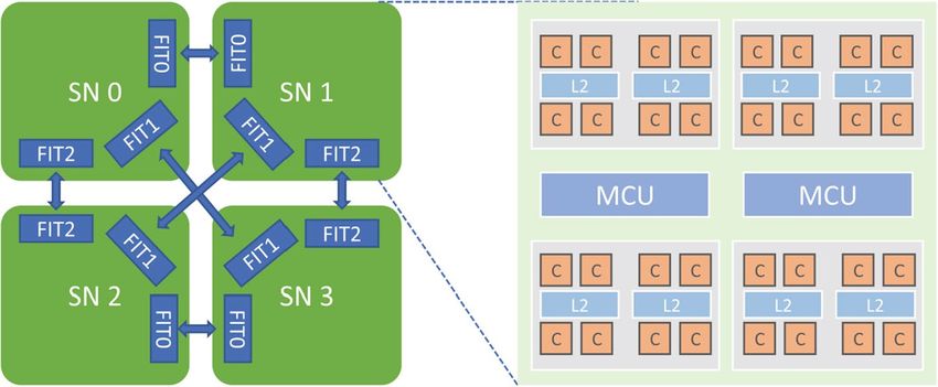
www.nature.com/scientificreports/
use a parallel programming framework to design neural network distributed computing methods that can give
full play to the computing power of high-performance platforms. In order to achieve an optimized design to give
full play to the high performance of the supercomputing platform, it is first necessary to perform corresponding
evaluation and tuning on the specific high-performance computing cluster. This paper evaluates and optimizes
the distributed training performance of neural networks on the Tianhe-3 Prototype platform.
The contribution of this paper is as follows:
• Designed a series of targeted experiments by considering three dimensions: neural network model, neural
network execution framework, and test pattern, in response to the unique architectural characteristics of the
Tianhe-3 prototype.
• The distributed framework of Pytorch was ported to the Tianhe-3 prototype and adapted to the Tianhe MPI.
• Different test strategies were designed and implemented for various cases such as single MTP node, single
FTP node, multiple MTP nodes, and multiple FTP nodes, respectively.
• A Dynamic Allreduce Algorithm communication optimization strategy is proposed for the gradient syn-
chronization process of distributed data parallel deep learning.
This paper is organized as follows: “Related work” section describes about distributed parallel deep learning
training in single and multi-node, “Key issues” section introduces mini-batch gradient descent, parallel model
in distributed environment, consistency computing model and the basic information of the Tianhe-3 proto-
type system, “Dynamic Allreduce algorithm” section introduces our proposed Dynamic Allreduce Algorithm,
“Experimental design” section presents our experimental design in terms of neural network model, neural net-
work execution framework and test model, “Experimental evaluation” section shows our experimental results in
the Tianhe-3 prototype using the experimental design in “Experimental design” section for single and multiple
nodes, and provides a detailed analysis of the extensibility, computation and communication overhead of the
algorithm, and finally, the full paper is summarised in “Conclusion” section.
Related work
With the increasing task scale and the deepening of network layers, the distributed training of the deep neural
network has experienced the development from a single node to multi node. On a single node, multi-core and
multi-core technology (GPU, MIC) is used for parallel acceleration; for large-scale deep neural network train-
ing tasks that cannot be completed by a single node, MPI or spark9 is usually used to complete the training of
the whole model through the distributed system. In the parallel acceleration training process, people focus on
using ASIC, FPGA, or c luster17, 25–28.
In terms of GPU acceleration, Raina et al.15 first proposed to use GPU to accelerate deep Boltzmann machine
(DBN); Yadan16 and others used four NVIDIA Geforce GTX Titan GPUs on a single server to realize the com-
bination of data parallelism and model parallelism; Li14 and others used a single Tesla k40c GPU to accelerate
DBN, and compared with Intel Core i7-4790k, it obtained 14–22× speedup the ratio in the pre-training process;
Bottleson et al.13 proposed an OpenCL accelerated Caffe framework for CNN network, and compared with Intel
CPU, it obtained 2.5–4.6× speedup after different optimization methods.
In terms of MIC acceleration, OpenMP parallel programming model is generally used. Olas et al.29 ran DBN
in native mode on Intel Xeon phi 7120p, and achieved 13.6× speedup compared with the serial version of Intel
Xeon e5-2695v2 CPU under 240 threads. Zlateski et al.30 proposed a 3D convolution algorithm, which achieved
near-linear speedup on Intel CPU and 90× speedup on 5110P. In terms of FPGA acceleration, Suda et al.27 has
implemented two kinds of networks, VGG and Alexnet on FPGA, among which VGG is 5.5× compared with
Intel i5-4590 3.3 GHz CPU. Zhang et al.28 implemented VGG network on FPGA, and the computing performance
of VGG network on Altera Arya 10 reached 1.79tops, and obtained 4.4× acceleration ratio compared with Intel
Xeon e5-1630v3 CPU. Utkuaydonat et al.26 implemented Alexnet network on FPGA, optimized the out of chip
memory bandwidth, and introduced the Winograd conversion method, and finally reached the peak performance
of 1382 GFLOPS when running on ARRIA 10.
In terms of Multi Nodes parallelization acceleration, deep neural network multi node parallelization is mainly
on the CPU cluster. The classic work includes Google’s dean et al. Who developed Google’s deep learning software
framework distbelief on the CPU cluster. Kaida song et al. Trained the DBN network with data parallel strategy
on the domestic supercomputer Taihu Light, and trained the MNIST data set on four computing nodes. The
performance achieved is 23 times higher than that of Intel Xeon e5-2420v22.2g C PU26. Ammar et al.designed
a distributed deep learning framework S-caffe with 12 nodes and 80 Tesla K80 GPUs using the method of col-
laborative design25. Fang Jiarui et al. Proposed Swcaffe, transformed and transplanted the Caffe framework to
Taihu Light, and obtained processing speed exceeding nvk40m GPU in some neural network structures17. Moritz
et al. Realized the combination of spark and Caffe, and improved the traditional synchronous SGD parallelization
mechanism by introducing control parameters to reduce the synchronization t imes18.
Testing and tuning supercomputers have always been an important and challenging topic in the HPC field.
Peng et al.19 implemented Amber parallel acceleration strategy for the molecular dynamics model on Tianhe-2
computer, realizing 25–33 times acceleration of the original program; Yifeng Xu et al.tested ZnO MOCVD
cavity numerical model on Tianhe-2 platform and the maximum acceleration ratio was 45. Zhu et al.24 studied
the distributed extension of Caffe, a deep learning framework, for the supercomputing platform of “Shenwei
Taihu Light”. They compared the distributed expansion method of parameter server and decentralized distrib-
uted expansion method under synchronous mode. Their experiments show that the decentralized distributed
extension method is more effective than the distributed extension method of parameter server in synchronous
mode. It has obvious advantages in the aspect of signal efficiency, and the communication performance can be
Scientific Reports | (2021) 11:20244 | https://doi.org/10.1038/s41598-021-98794-z 2
Vol:.(1234567890)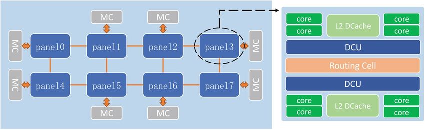
www.nature.com/scientificreports/
improved by 98 times for a specific model. you et al.23 tested and analyzed the computing performance of linear
algebraic kernel for Tianhe-3 Prototype, and compared the performance of MTP and FTP on Tianhe-3 Prototype
and KNL processor for comparison. Li et al.22 proposed a heuristic topology-aware mapping algorithm Kohtma
to evaluate and improve the communication performance of Tianhe-3 Prototype. Their experiments show that
this method can greatly reduce the communication cost.
Key issues
In this section, we mainly introduce four key points of distributed training in this paper: small-batch gradient
descent, parallel model in a distributed environment, consistency computing model and Tianhe-3 Prototype.
Mini‑batch gradient descent. In the process of deep neural network training, a very important task is to
solve the cost function (that is, to solve the weight of each layer of the network). At present, the most commonly
used optimization algorithm is a gradient descent algorithm. The core of the algorithm is to minimize the objec-
tive function by iterative convergence. In each iteration, the corresponding parameter value of each variable is
updated according to the objective function in the opposite direction of the variable gradient. Among them, the
parameter learning rate and the target optimization index determine the number of iterations to reach the mini-
mum value. There are three different variants of the gradient descent method: Batch Gradient Descent (BGD),
Stochastic Gradient Descent (SGD), and Mini Batch Gradient Descent (MBGD, as shown in Algorithm 1). BGD
can ensure that it converges to the global optimal value of a convex function or local optimal value of a noncon-
vex function, but each update needs to be solved on the whole data set, so the speed is slow. Even for large data
sets that cannot be stored in memory, this method can not be used, and the model can not be updated in the
form of a line. Each update of SGD only solves the gradient of one sample in the data set and runs Compared
with BGD, SGD is easy to fall into local minima, and the convergence process is more fluctuating. MBGD com-
bines the advantages of the above two methods. In each update, MBGD solves a batch of data composed of n
samples to make the convergence process more stable. It is usually the preferred algorithm for training neural
networks. Therefore, in this paper, MBGD is chosen as the method to solve the cost function.
Parallel model in distributed environment. There are two main methods for the parallel of deep neural
network: model parallel and data parallel20. Model parallelism refers to the decomposition of network model to
each computing device, and the training is performed by the cooperation between devices. Model parallelism is
more suitable for large models with many levels, few dependencies between levels, and where a single compute
node cannot complete the entire network training. Data parallelism refers to the segmentation of training data,
and the parallel training of multi segmented data is conducted by using multiple model examples. As shown in
Fig. 1, in the data parallel training process, each node uses its own data to train the entire network for one epoch,
then perform gradient averaging and update the local weights and move on to the next epoch. ω represents the
wieght value and η represents the learning rate. The parameter exchange is completed by parameter server or
by using decentralized communication mechanisms such as all-reduce. In MSGD, the data is processed in n
samples as batches. Since most operators are independent from n, the direct way to parallelize is to allocate small
batches of samples between multiple computing resources (processor cores or devices) to perform work. This
method (initially called pattern parallelism, and input samples as patterns) can be traced back to the first practi-
cal implementation of artificial neural networks. It can be considered that the use of micro-batch in gradient
descent is initially driven by data parallelism. Farber and Asanović31 use multiple vector accelerator micropro-
cessors (Spert II) to perform error reverse propagation in parallel to speed up neural network training. In order
Scientific Reports | (2021) 11:20244 | https://doi.org/10.1038/s41598-021-98794-z 3
Vol.:(0123456789)www.nature.com/scientificreports/
Figure 1. Deep neural network data parallel.
to support data parallelism, they proposed a delayed gradient update version called “bundle mode”, in which the
gradient was updated several times before updating the weight, essentially equivalent to MSGD.
Raina et al. First mapped DNN computing to data parallel architecture (such as GPU). They focus on training
deep belief networks and map the unsupervised training process to GPU by running MSGD. Their training results
on the restricted Boltzmann machine increased the CPU speed by 72.6 times. Nowadays, most deep learning
frameworks support deep data parallelization. They can use a single GPU (CPU) or a cluster of multiple GPU
(CPUs) nodes. With MapReduce, parallel tasks can be scheduled to multiple processors and distributed envi-
ronments. Prior to these works, researchers have studied the potential scale of MapReduce for various machine
learning problems, including neural networks, which promotes the need to shift from single-processor learning
to distributed storage systems.
For the Pytorch training platform used in this article, it supports data parallelism, training a copy of the
model independently on each device. When updating the parameters, the gradient of each device is transmitted
to the parameter device for parameter updating. The 1bit SGD algorithm is supported to reduce the amount of
data transmitted.
Consistency computing model. With the increasing amount of data, a single machine can not store all
the data, so a distributed optimization algorithm has become a hot spot. Researchers have proposed parallel
optimization algorithms based on parallel computing models such as bulk synchronous parallel (BSP)32, delay
synchronization (SSP)33, and asynchronous (ASP)33.
The global synchronous parallel computing model BSP is composed of a group of distributed processors with
local memory and roadblocks supporting global synchronization between all processing units. The synchro-
nous update process is as follows: multiple processor units update the model in the same iteration round. After
completing a round of iteration, the multiprocessor units wait synchronously at the master node according to
the roadblock mechanism. The master node updates the model uniformly and sends the updated parameters to
each processor unit for a new round of iteration. Common BSP model systems include mahout34, spark34, etc.
The asynchronous parallel computing model ASP is composed of a distributed processor with local memory
and a total node managing global parameters. The asynchronous update process is: each node updates the model
on the master node in an asynchronous manner. Combined with the data division, it can be explained that: each
node calculates all model parameters with local data. After one round of calculation, the node can update the
model parameters at the master node, and then get the latest global parameters from the master node for the next
round of updating. Each node does not need to wait for each other. However, there is no limit on the number
of iterations of each node, which will result in the final non-convergence. In order to solve the instability of the
ASP model, the following delay synchronization parallel computing model is proposed.
Delay synchronous parallel computing model SSP is composed of a distributed processor with local memory,
total node and delay parameter (stale). The semi asynchronous update the process is: each node updates the
model on the master node with different rounds, but with a little restriction, the iteration rounds of the param-
eters of the fastest and slowest nodes should not be greater than stale, so that the slow nodes can not only slow
Scientific Reports | (2021) 11:20244 | https://doi.org/10.1038/s41598-021-98794-z 4
Vol:.(1234567890)www.nature.com/scientificreports/
Figure 2. FT2000+ processor architecture.
Figure 3. MT2000+ processor architecture.
Specifications FT-2000+ MT-2000+
Nodes 128 512
Cores in a node 32 32
Hardware Frequency 2.4 GHZ 2.0 GHZ
Memory 64 GB 16 GB
Interconnect bandwidth 200 Gbps 200 Gbps
OS Kylin 4.0-1a OS with kernel v4.4.0
File system Lustre
Software MPI MPICH v3.2.1
Compiler GCC v4.9.1/v4.9.3
Supported libraries Boost, BLAS, OpenBLAS, Scalapack, etc.
Table 1. Basic situation of Tianhe-3 prototype system.
down the running speed of the whole system but also ensure the final convergence of the model parameters.
Common SSP model systems include P etuum35, deep learning system20, 36, 37, etc.
Tianhe‑3 prototype.
As shown in Figs. 2 and 3, the processors used in the Tianhe-3 Prototype include FT-2000+ (FTP) and MT-2000+
(MTP). In the official website of Tianjin Supercomputing Center and Feiteng Company, as well as published
papers, you can know that FTP contains 64 FTC662 processor cores with armv8 architecture, the main frequency
is 2.2-2.4GHZ, the on-chip 32MB secondary cache is integrated, which can provide 204.8GB/s memory access
bandwidth and the typical working energy consumption is about 100W; while the MTP processor, It contains
a total of 128 customized processor cores, organized into 4 super nodes, the main frequency is up to 2.0GHZ,
and the entire processor consumes 240W. In addition, both processors support 128-bit SIMD vector or scalar
floating point operations, which is critical for deep learning. The processor architecture of FTP and MTP is
shown in the figure below:
In Tianhe-3 Prototype, as shown in Table 1 below, FTP and MTP are both divided into 32 cores as one com-
puting node. The purpose of doing so may be to provide more computing nodes to meet complex computing
Scientific Reports | (2021) 11:20244 | https://doi.org/10.1038/s41598-021-98794-z 5
Vol.:(0123456789)www.nature.com/scientificreports/
Figure 4. Pytorch distributed Allreduce method.
Figure 5. Recursive halving and doubling, butterfly and ring Allreduce.
t asks23. The computing nodes are managed and allocated by the batch scheduling system. In FTP, 32 cores share
64g of memory, while in MTP, 32 cores share 16g of memory. They all come with Kylin 4.0-1a operating system
with kernel v4.4.0.
In addition, the Prototype cluster interconnection technology designed and implemented by the University
of Defense Science and technology provides 200gbps bidirectional interconnection bandwidth. The Prototype
uses Lustre for distributed file system management. At the same time, the Prototype provides multiple versions
of MPI compiler implementation, including MPICH 3.2.1 (supports gcc4.9.3, gcc8.2.0, and gcc8.3.0) and an
openmpi4.0.0 which is still in the debugging stage. In addition, lammps, GROMACS, and other scientific com-
puting applications are preset.
Unfortunately, the Prototype does not provide development frameworks for deep neural networks such
as Caffe, Pytorch, Tensorflow, etc. Therefore, the work of this article first starts with the transplantation of the
Pytorch framework.
Dynamic allreduce algorithm
In the distributed data parallel deep learning training process, each node has to perform gradient averaging after
each small batch of data training to obtain the training results of each node to update the network weights, and
this process is now often done using parameter servers or Allreduce operations for aggregate communication.
The existing Pytorch distributed underlay uses an all-broadcast-like Allreduce strategy as shown in Fig. 4 (We
can use it easily by calling the torch.distributed.all_reduce() API.). Although this strategy can alleviate the prob-
lem that parameter server models are prone to single-point-failure communication bottlenecks, this approach
increases the amount of communication data by a factor of n-1 (n is the number of nodes), and at larger data
blocks (as the neural network model becomes more complex, the model gradient of updated data increases) are
prone to delay jitter.
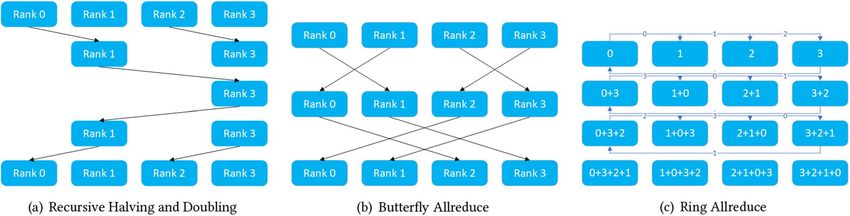
As a result, we combine the architectural features of Tianhe-3 and introduce the three most commonly used
current pooled communication underlying strategies of Recursive Halving and Doubling, Butterfly and Ring
AllReduce. As shown in Fig. 5, different strategies show different performance variations when exchanging
data size, interconnection method between nodes, sending and receiving buffer size, node processor type, etc.
Generally, with the same communication bandwidth, the communication throughput will show a non-linear
variation with the size of the communication data block, and the communication speed will be fastest when the
size of the model matches the size of the data volume corresponding to the maximum value of the communica-
tion throughput. In the past, people normally choose based on experience, but this requires researchers to have
sufficient knowledge of the underlying communication mechanisms and implementations as well as the size of
the exchanged data, which is often not a necessary skill for deep learning researchers.
In light of this, we take full advantage of distributed training to design and implement a probe mechanism
that allows users to automatically select the most suitable underlying communication method without the need
to know the underlying implementation of the communication.
As shown in Algorithm 2 below, after all compute nodes have completed data preprocessing, they commu-
nicate using the original Allreduce, Recursive Halving and Doubling, Butterfly, Ring AllReduce, and Parameter
Server when executing the first 5 batch synchronization gradients, respectively, and the total communication time
for each strategy is saved in the local probe. In each subsequent training round, the gradient averaging is done
Scientific Reports | (2021) 11:20244 | https://doi.org/10.1038/s41598-021-98794-z 6
Vol:.(1234567890)www.nature.com/scientificreports/
Model Conv layers FC layers Dataset
LeNet 2 2 Mnist
AlexNet 5 3 Cifar-10
VGG16 13 3 Cifar-10
ResNet18 17 1 Cifar-10
Table 2. Neural network configuration.
using the communication strategy with the shortest communication time obtained from the above four probes.
At the same time, if the number of neurons in each layer of the neural network model varies greatly, resulting in
uneven amounts of simultaneous gradient data in each layer, it is also possible to probe deeper into each neural
network layer and specify a specific underlying communication strategy for each layer of the neural network
gradient averaging operation. Specifically, if the underlying communication policy needs to be optimised layer
by layer, we simply create a probe for each layer as described in Algorithm 2. Similar to the optimisation for the
whole network, the communication times of the different underlying communication policies are stored in the
probes of each layer separately, and then each layer probe selects the policy with the shortest communication
time in its layer as the underlying communication policy for gradient synchronisation in the subsequent train-
ing process of each layer.
Experimental design
We propose a targeted experimental design by considering three dimensions: neural network model, neural
network execution framework and test pattern to fully test the performance of the Tianhe-3 prototype in dis-
tributed training of deep neural networks.
Neural network model. To fully test the performance of the Tianhe-3 prototype in distributed training
of deep neural networks, As shown in Table 2, we first selected a modified version of the LeNet model to test in
detail the performance of the Tianhe-3 single-node and multi-node implementations when working on image
classification of the Minist dataset, which contains two convolutional layers (conv layers), two pooling layers,
three activation layers, and two fully connected layers(fc layers). The first convolutional layer, with an input
channel count of 1 and an output channel count of 10, has a convolutional kernel size of 5x5, a stride size of 1,
and zero padding. The second convolutional layer has 10 input channels and 20 output channels, and the rest
is the same as the first convolutional layer. Both pooling layers use the maximum pooling method. All three
activation functions use the relu function. The drop_out optimization method is also used for the model. Subse-
quently, we also verify the scalability of Tianhe-3 by using the classical AlexNet, VGG16 and ResNet18 models
for image recognition on the Cifar-10 dataset. We use a fixed batch size of 128 for mini-batch stochastic gradi-
ent descent, and the number of training samples per batch for each training process is 128/n (n represents the
number of processes involved in training).
Neural network execution framework. We first ported the P
ytorch38 distributed deep neural network
training framework to the Tianhe-3 prototype platform. Pytorch has a fairly simple, efficient, and fast framework
that is designed to pursue minimal packaging, conform to the human mind, and allow users to focus on imple-
menting their ideas as much as possible. Pytorch provides a rich library of deep learning kernels, which allows
us to quickly and easily build deep learning networks and implement training and inference, for example, by
calling the Torch.nn API to easily implement Conv, Pooling, Linear, Batchnorm, Dropout and other basic opera-
tions commonly used in deep learning. Pytorch supports the use of MPI, GLOO or NCCL (Nvidia GPUs only)
underlying communication frameworks, and we used four MTP nodes to train 10 rounds of the task of classify-
ing Cifar-10 images in AlexNet networks using each of the two frameworks, and the results are shown in Table 3
below. The training time using the GLOO framework is more than five times that using the MPI framework, so
Scientific Reports | (2021) 11:20244 | https://doi.org/10.1038/s41598-021-98794-z 7
Vol.:(0123456789)www.nature.com/scientificreports/
Communication framework Training time (mins)
MPI 141.55
GLOO 732.94
Table 3. AlexNet using GLOO framework or MPI framework to classify the Cifar-10.
we chose MPI, which is more suitable for Tianhe-3, as the distributed underlying communication architecture.
Meanwhile, this determines that we can only deploy pytorch on Tianhe-3 using the source installation.
The datasets we use for training are the Mnist dataset and the Cifar-10 dataset, a very classical dataset in the
field of machine learning, consisting of 60,000 training samples and 10,000 test samples, each of which is a 28×28
pixel grayscale handwritten digital image. CIFAR-10 is a small dataset for recognizing pervasive objects compiled
by Hinton’s students Alex Krizhevsky and Ilya Sutskever, a small dataset for identifying pervasive objects. A total
of 10 categories of RGB color images are included: airplanes, cars, birds, cats, deer, dogs, frogs, horses, boats, and
trucks. The size of the images is 32×32, and there are 50,000 training images and 10,000 test images in the dataset.
Test model. Tianhe-3 Prototype has two different processor nodes: MT-2000+ and FT-2000+. This paper
designs MT-2000+ and FT-2000+ single node and multi-process parallel training tasks, MT-2000+ multi-node
and multi-process distributed training tasks and FT-2000+ multi-node and multi-process distributed training
tasks to a comprehensive evaluation of single-node parallel training performance and the scalability of multi-
node distributed training on the Tianhe-3 prototype.
We can get the Scale-up capability of the Tianhe-3 prototype through a single-node multi-process training
design, the Scale-out capability through a multi-node single-process training design, and finally, the capability
under both Scale-up and Scale-out through a multi-node multi-process training design.
In order to ensure the robustness of the data, all experimental results in this paper are the arithmetic mean
after five tests.
Experimental evaluation
In this section, according to the experimental scheme designed in the previous section, as shown from Figs. 6, 7,
8, 9, 10, 11, experiments are carried out for MTP, FTP single node and multi nodes, and the experimental results
are summarized and analyzed, and the reasons for the experimental results are explained. Training times for all
experiments are counted in minutes.
Single node performance. In order to fully explore the performance on different multicore processor
nodes of MT2000+ and FT2000+, we used a minimum of 1 process to a maximum of 32 processes on one node
of two different processors (according to the architectural characteristics of Tianhe-3, a node uses a maximum
of 32 processor cores, wherein our experiments MTP can only use a maximum of 20 processes, otherwise it will
lead to memory insufficient resources) to classify the Minist dataset using the LeNet model described in the
previous section. We adopt a distributed training strategy with data parallelism, an Allreduce communication
strategy, and use a strict consistency synchronization protocol (BSP) while shuffling the data on the training set
and distributing it evenly over the processes. To ensure consistent training accuracy when testing across multiple
processes, we ensure that the same random number is obtained for each experiment by setting a fixed random
seed at the beginning of the program.
The accuracy of training in a single MT2000+ node with 10 iterative rounds using 1–20 processes is shown
in Fig. 6a. The accuracy results obtained with different numbers of processes are 97.82% on average, and the
extreme difference is only 0.04%, which proves the accuracy and robustness of distributed training in a single
node of MT2000+. As shown in Fig. 6b, the corresponding total training time is 4.6025 mins when the number
of processes is 2, and then the overall training time basically increases with the number of processes (decreases
when the number of processes is 8), reaching a maximum of 37.0641 mins when the number of processes is 20;
meanwhile, it is found that when the number of processes is a power of 2, the training results are better than
the adjacent processes (this is because when The number of nodes that are not a power of 2 when performing
parameter synchronization first performs an additional operation to scale the number of nodes to a power of 2
increasing the additional training time).
In a single FT2000+ node, 1–32 processes are used for 10 iterations, and the accuracy of training is shown
in Fig. 6c. The average accuracy of different processes is 97.81%, and the range is only 0.035%, which proves
the accuracy and robustness of ft2000 + single node distributed training. According to the total training time,
as shown in Fig. 6d, the shortest training time is 3.9958 minutes when the number of processes is 2, and then
the overall training time increases with the increase of the number of processes (decreases when the number of
processes is 8), and reaches the maximum of 52.0821 minutes when the number of processes is 32. Similar to
the result in MTP, when the number of processes we use is a power of 2, the training result is obviously better
than the selection of adjacent processes.
Multi nodes performance. As shown in Fig. 7a and c, in the MT2000+ multi-node training process, when
the total number of nodes used is less than 8, the shortest training time can be achieved when the number of
processes is twice the number of nodes, while Accuracy remains basically the same; when the number of nodes
Scientific Reports | (2021) 11:20244 | https://doi.org/10.1038/s41598-021-98794-z 8
Vol:.(1234567890)www.nature.com/scientificreports/
Figure 6. MT2000+ and FT2000+ single node training accuracy and training time.
is greater than or equal to 8, the shortest training time can be achieved while minimizing the Accuracy value by
choosing the number of processes consistent with the number of nodes.
As shown in Fig. 7b and d, in the FT2000+ multi-node training process, when the total number of nodes used
is less than or equal to 8, similar to MTP, when the number of processes is twice the number of nodes, the shortest
training time can be achieved while Accuracy remains basically constant, but this time will gradually approach
the training time when the number of processes is equal to the number of nodes as the number of nodes increases.
Extensibility verification. To verify the scalability of the Tianhe-3 supercomputer, we also extended the
training scheme in the previous section to typical AlexNet, VGG16 and ResNet18 models, and completed the
image recognition task on the Cifar-10 dataset using 1-32 FTP and 1-128 MTP, respectively. The training time
for different number of nodes is shown in Fig. 8. The training time decreases with the increase of the number of
nodes, showing the good scaling capability of Tianhe-3.
Overall result analysis. Based on the test results in the previous section, we found that in the performance
of single nodes, both FTP and MTP, the results are better when using a power of 2 for the number of processes
than the neighboring process number choices (less training time to obtain the same training accuracy). After ten
epochs, both processor single nodes achieve optimal training results at a number of processes of 2. At this point,
the classification accuracy of FTP is slightly higher than that of MTP by 0.03%, and the single simultaneous
training time is reduced by about 13%. When using single nodes, FTP training was faster than MTP regardless
of the number of processes used. In the multi-node performance, when the number of nodes used in FTP is less
than 16, the results are consistent with those of a single node, and using twice the number of processes as the
number of nodes can achieve the shortest training time while the classification accuracy is basically constant. In
MTP multi-node training, after the number of nodes is greater than or equal to 8, using the same number of pro-
cesses as the number of nodes can achieve the shortest training time without losing training accuracy. In addi-
tion, we also find that using more nodes, when the number of processes used is the same because more processor
cores can be used, must be able to achieve a shorter training time without losing the classification accuracy again.
The advantages and disadvantages of the various architectures are shown in Table 4.
The difference in training performance between single-node and multi-node training with different numbers
of processes is explained in the next section by analyzing the specific computation time and communication time.
A plain reason is that when using single-node training, the computational performance of the nodes is better
utilized with two processes than with a single process, but as the number of processes continues to increase,
Scientific Reports | (2021) 11:20244 | https://doi.org/10.1038/s41598-021-98794-z 9
Vol.:(0123456789)www.nature.com/scientificreports/
Figure 7. MT2000+ and FT2000+ multi nodes training loss and training time.
4
AlexF AlexM V GG16F V GG16M Res18F Res18M
3.5
LgTime (mins)
3
2.5
2
1.5
1
1 2 4 8 16 32 64 128
Number of Nodes
Figure 8. AlexNet, VGG16, and ResNet18 trainig time.
the loss of inter-process communication overhead and the additional overhead caused by inter-process access
conflicts outweigh the computational performance gain from increasing the number of processes, resulting in
an overall increase in training time; the reason is the same as in single-node when the number of MTP nodes is
less than 8 and the number of FTP nodes is less than or equal to 16. When the number of FTP nodes is less than
or equal to 16, the reason is the same as in a single node; when the number of nodes continues to increase, even
twice the number of processes causes the loss of communication overhead to outweigh the gain in computational
performance, so using one process per node is the best choice in this case.
Computing and communication cost analysis. Further, in order to fully investigate the reasons for the
above experimental results, we divided the whole experiment into computation time T1 (which mainly includes
the computation overhead of forward and backward propagation of the neural network model and loss value
calculation) and communication time T2 (which mainly refers to the communication overhead of global gradi-
Scientific Reports | (2021) 11:20244 | https://doi.org/10.1038/s41598-021-98794-z 10
Vol:.(1234567890)www.nature.com/scientificreports/
Figure 9. MT2000+ and FT2000+ single node computing and communication time.
Distributed training architecture Advantages Disadvantages
Single-node multi-process (scale-up) Simple, cheap Slow
Multi-node single-process (scale-out) Simple, medium speed Expensive
Multi-node multi-process (both) Fast Expensive, complicated
Table 4. The advantages and disadvantages of the various architectures.
Figure 10. MT2000+ and FT2000+ single node computing time.
ent update using Allreduce), and the total time T is the sum of the above two overheads. In FTP and MTP single
nodes, the two computational overheads and communication overheads are shown in Fig. 9.
T = T1 + T2 (1)
Among them, as shown in Fig. 10, the computational overhead T1 is the overhead that must be paid in order
to train the network. As the number of processes increases, the number of training subsets assigned to a single
process will decrease, and thus the overhead of forward-propagation and backward-propagation computational
operations (including convolution, pooling, activation operations, local gradient update, loss value update, etc.)
of the neural network required in a single process will decrease; however, at the same time, as the However, at
the same time, as the number of processes increases, the Cache hit rate of each process will significantly decrease
and the access conflict will significantly increase according to the shared memory and shared Cache architecture
features of the Tianhe-3 prototype. When the number of processes is first incremented, the impact of the former
is greater than the latter, so the computation time will increase as the number of processes increases; subsequently,
as the number of processes continues to increase, the impact of access conflicts will be much greater than the
gain in computation overhead, so the computation time will rise significantly with the increase in the number
Scientific Reports | (2021) 11:20244 | https://doi.org/10.1038/s41598-021-98794-z 11
Vol.:(0123456789)www.nature.com/scientificreports/
Figure 11. MT2000+ and FT2000+ single node communication time.
of processes. Therefore, this leads to the trend that the computation overhead decreases and then increases with
the increase of the number of processes.
Similarly, as shown in Fig. 11, the communication overhead T2 is the loss on the path in order to synchronize
the weights in the neural network, and it can be calculated using the following equation:
T2 = K × log2 N × (α + S/B + S × C) (2)
Among them, α represents the communication delay between the two processes. It will vary with the dis-
tribution and relative distance of the processor cores on the chip. Processor cores sharing the same cache will
communicate significantly faster than those sharing only the same shared memory, while those sharing the same
shared memory will communicate significantly faster than those using different shared memory but within the
same node, and those between two different nodes will communicate the slowest. S (ize) represents the size of
the data block contained in each process when performing All-reduce operations, B (andwidth) represents the
communication bandwidth between the two processes, and C (omputing) represents the computing overhead
per byte (note that this Part of the computing cost refers to the computing cost in the All-reduce process, not
the computing cost mentioned in the previous section), N (numbers) represents the number of all processes
that communicate, and K represents the number of All-reduce operation. In our experiment, the Mnist data set
used has a total of 60,000 instances, and the Batchsize we choose is fixed at 128. Then every round of training is
performed, the number of All-reduce operations required is fixed, as:
K = 60000/128 (3)
Although the number of processes involved in each iteration is different, the size of the data block that a
single process interacts with is the size of the weight W of the constant neural network, which is counted as W,
S=W (4)
Therefore, formula (1) can be rewritten as:
T2 = 458.75 × log2 N(α + W/B + W × C) (5)
Therefore, it can be seen from the above formula that when the communication bandwidth and the calcula-
tion cost per bit are determined, the overall communication time is only related to the number of processes
and the communication delay between the two processes. Besides, when the number of processes is odd, the
communication overhead of each batch will increase by 1 unit time, so the total communication overhead time
when the number of processes is odd is:
(6)
T2 = 468.75 × log2 N(α + W/B + W × C) + 1
Therefore, with the exception of the FTP single-node experiment, in all other test scenarios, the total com-
munication time increases with the increase of the number of processes, because the change in communication
delay increases with the number of processes when the number of processes is small. There is little change, so the
total communication time T2 in the above formula is mainly affected by the number of processes N. T2 increases
with the increase of N, but as N increases, the magnitude of the increase of T2 decreases. Consistent with the
trend of the logarithmic curve. Further, this article found that in the training scenario of FTP single node, when
the number of processes exceeds 20, the overall communication time will decrease as the number of processes
increases, because when the number of processes is relatively large, the communication delay α and the com-
munication bandwidth B between processes will become complicated and cannot be generalized. Therefore, the
calculation method of the above communication delay should be described as:
Scientific Reports | (2021) 11:20244 | https://doi.org/10.1038/s41598-021-98794-z 12
Vol:.(1234567890)www.nature.com/scientificreports/
N
T2 = 468.7 × log2 (αi + W/Bi + W × C) + 1 (7)
i=1
It is found from the experiment that according to the above formula, when the number of processes continues
to increase, the overall communication delay between the processes decreases and the overall communication
bandwidth increases, resulting in a decrease in the total communication time.
Conclusion
We evaluate the distributed training performance of the Tianhe-3 prototype for deep neural networks using the
improved LeNet model, the classical AlexNet, VGG16, and ResNet18 models under our own ported pytorch
distributed framework and propose a dynamic selection algorithm for the underlying communication mecha-
nism. Our results can be used to guide the software and hardware design of Tianhe-3 as it moves toward E-class
computing. For a comprehensive evaluation and illustration of the results, we design comprehensive and detailed
experiments for single-node and multi-node clusters of FTP and MTP, respectively, providing software developers
and hardware architects with multiple perspectives for future performance optimization.
In addition, we compare the performance of FTP and MTP processors, which shows the advantages and
disadvantages of different processor architecture designs. It is hoped that we will provide a reference to the HPC
community and Tianhe-3 developers to benefit the Chinese E-class supercomputer program, thus opening the
way for the pursuit of E-class supercomputer development. In future work, we hope to combine the hardware
features of the Tianhe-3 prototype compute nodes and the characteristics of the network topology to perform
finer-grained tuning of the existing neural network distributed training framework structure on more platforms
besides Pytorch to better exploit the potential computational power of the Tianhe-3 prototype.
Received: 18 May 2021; Accepted: 14 September 2021
References
1. Lecun, Y., Bengio, Y. & Hinton, G. Deep learning. Nature 521(7553), 436 (2015).
2. Deng, L. et al. Recent advances in deep learning for speech research at Microsoft. In IEEE International Conference on Acoustics
(2013).
3. Krizhevsky, A., Sutskever, I. & Hinton, G. ImageNet classification with deep convolutional neural networks. Adv. Neural Inf. Proc.
Syst. 25(2), 1097–1105 (2012).
4. Chen, C. et al. DeepDriving: Learning Affordance for Direct Perception in Autonomous Driving. 1505.00256 [cs.CV] ( 2015).
5. Esteva, A. et al. Dermatologist-level classification of skin cancer with deep neural networks. Nature 542(7639), 115–118 (2017).
6. Silver, D. et al. Mastering the game of Go with deep neural networks and tree search. Nature 529(7587), 484–489 (2016).
7. Lee, H. et al. Unsupervised feature learning for audio classification using convolutional deep belief networks. Adv. Neural Inf.
Process. Syst. 22, 1096–1104 (2009).
8. Li, F. -F., Karpathy, A., & Johnson, J. Stanford CS Class CS231n: Convolutional Neural Networks for Visual Recognition (2017).
9. Sze, V., Chen, Y. H., Yang, T. J. & Emer, J. S. Efficient processing of deep neural networks: A tutorial and survey. Proc. IEEE 105(12),
2295–2329 (2017).
10. Esser, S. K. et al. From the cover: Convolutional networks for fast, energy-efficient neuromorphic computing. Proc. Natl. Acad.
Sci. U. S. A. 113(41), 11441 (2016).
11. Mathieu, M., Henaff, M., & LeCun, Y. Fast training of convolutional networks through ffts. arXiv preprint arXiv:1312.5851 (2013).
12. Salehi, M. A. et al. Stochastic-based robust dynamic resource allocation for independent tasks in a heterogeneous computing
system. J. Parallel and Distrib. Comput. 97(2016), 96–111 (2016).
13. Bottleson, J. et al. clcaffe: Opencl accelerated caffe for convolutional neural networks. In 2016 IEEE International Parallel and
Distributed Processing Symposium Workshops (IPDPSW). IEEE, 50–57 (2016).
14. Li, T. et al. Optimized deep belief networks on CUDA GPUs. In 2015 International Joint Conference on Neural Networks (IJCNN).
IEEE, 1–8 (2015).
15. Raina, R., Madhavan, A., & Ng, A. Y. Large-scale deep unsupervised learning using graphics processors. In Proceedings of the 26th
Annual International Conference on Machine Learning. 873–880 (2009).
16. Yadan, O. et al. Multi-gpu training of convnets. arXiv preprint arXiv:1312.5853 (2013).
17. Li, L. et al. swcaffe: A parallel framework for accelerating deep learning applications on sunway taihulight. In 2018 IEEE Interna-
tional Conference on Cluster Computing (CLUSTER). IEEE, 413–422(2018).
18. Moritz, P. et al. Sparknet: Training deep networks in spark. arXiv preprint arXiv:1511.06051 (2015).
19. Peng, S. et al. High-scalable collaborated parallel framework for large-scale molecular dynamic simulation on Tianhe-2 super-
computer. IEEE/ACM Transactions on Computational Biology and Bioinformatics (2018).
20. Dean, J. et al. Large scale distributed deep networks. Adv. Neural Inf. Process. Syst. 25, 1223–1231 (2012).
21. He, X. et al. Testing high performance numerical simulation programs: experience, lessons learned, and open issues. In Proceedings
of the 29th ACM SIGSOFT International Symposium on Software Testing and Analysis. 502–515 (2020).
22. Li, Y. et al. OHTMA: An optimized heuristic topology-aware mapping algorithm on the Tianhe-3 exascale supercomputer proto-
type. Front. Inf. Technol. Electronic Eng. 21(6), 939–949 (2020).
23. You, X. et al. Performance evaluation and analysis of linear algebra kernels in the prototype tianhe-3 cluster. In Asian Conference
on Supercomputing Frontiers. Springer, 86–105 (2019).
24. Zhu, C. Liu, X. & Fang, J. Research on distributed extension of Caffe based on “light of Taihu Lake” in Shenwei. Comput. Appl.
Softw. (2020).
25. Awan, A. A. et al. S-caffe: Co-designing mpi runtimes and caffe for scalable deep learning on modern gpu clusters. In Proceedings
of the 22nd ACM SIGPLAN Symposium on Principles and Practice of Parallel Programming. 193–205 (2017).
26. Song, K. et al. Restricted Boltzmann machines and deep belief networks on sunway cluster. In 2016 IEEE 18th International
Conference on High Performance Computing and Communications; IEEE 14th International Conference on Smart City; IEEE 2nd
International Conference on Data Science and Systems (HPCC/SmartCity/DSS). IEEE, 245–252 (2016).
27. Suda, N. et al. Throughput-optimized OpenCL-based FPGA accelerator for large-scale convolutional neural networks. In Proceed-
ings of the 2016 ACM/SIGDA International Symposium on Field-Programmable Gate Arrays. 16–25 (2016).
28. Zhang, J., & Li, J. Improving the performance of OpenCL-based FPGA accelerator for convolutional neural network. In Proceedings
of the 2017 ACM/SIGDA International Symposium on Field-Programmable Gate Arrays. 25–34 (2017).
Scientific Reports | (2021) 11:20244 | https://doi.org/10.1038/s41598-021-98794-z 13
Vol.:(0123456789)www.nature.com/scientificreports/
29. Olas, T. et al. Adaptation of deep belief networks to modern multicore architectures. In International Conference on Parallel Pro-
cessing and Applied Mathematics. 459–472 (Springer, 2015)
30. Zlateski, A., Lee, K. & Seung, H. S. Scalable training of 3D convolutional networks on multi-and many-cores. J. Parallel and Distrib.
Comput. 106, 195–204 (2017).
31. Farber, P., & Asanovic, K. Parallel neural network training on multi-spert. In Proceedings of 3rd International Conference on Algo-
rithms and Architectures for Parallel Processing. IEEE, 659–666 (1997).
32. Loulergue, F., Gava, F., & Billiet, D. Bulk synchronous parallel ML: Modular implementation and performance prediction. In
International Conference on Computational Science. 1046–1054 (Springer, 2005).
33. Eric P, X., Qirong, H., Xie, P. & Wei, D. Strategies and principles of distributed machine learning on big data. Engineering 2(2),
179–195 (2016).
34. Li, M. et al. Scaling distributed machine learning with the parameter server. In 11th {USENIX}Symposium on Operating Systems
Design and Implementation ( {OSDI} 14). 583–598 (2014).
35. Ho, Q. et al. More effective distributed ml via a stale synchronous parallel parameter server. Adv. Neural Inf. Process. Syst. 1223–1231
(2013).
36. Abadi, M. et al. Tensorflow: A system for large-scale machine learning. In 12th{USENIX}Symposium on Operating Systems Design
and Implementation ({OSDI} 16). 265–283 (2016).
37. Chen, T., et al. Mxnet: A flexible and efficient machine learning library for heterogeneous distributed systems. arXiv preprint arXiv:
1512.01274 (2015).
38. Mccaffrey, J. Introduction to PyTorch on windows. Msdn Mag. 34(1), 16–23 (2019).
Author contributions
J.W., Conceptualization, Methodology, software, Investigation, Writing—original draft. Validation. X.Z.,
Resources, Funding acquisition, Project administration, Supervision. Z.J., Data curation, Validation. J.L., For-
mal analysis. Z.W., Investigation.
Funding
This research has been supported by the China National Key R&D Program during the 13th Five-year Plan
Period (Grant No. 2018YFB1700405).
Competing interests
The authors declare no competing interests.
Additional information
Correspondence and requests for materials should be addressed to X.Z.
Reprints and permissions information is available at www.nature.com/reprints.
Publisher’s note Springer Nature remains neutral with regard to jurisdictional claims in published maps and
institutional affiliations.
Open Access This article is licensed under a Creative Commons Attribution 4.0 International
License, which permits use, sharing, adaptation, distribution and reproduction in any medium or
format, as long as you give appropriate credit to the original author(s) and the source, provide a link to the
Creative Commons licence, and indicate if changes were made. The images or other third party material in this
article are included in the article’s Creative Commons licence, unless indicated otherwise in a credit line to the
material. If material is not included in the article’s Creative Commons licence and your intended use is not
permitted by statutory regulation or exceeds the permitted use, you will need to obtain permission directly from
the copyright holder. To view a copy of this licence, visit http://creativecommons.org/licenses/by/4.0/.
© The Author(s) 2021
Scientific Reports | (2021) 11:20244 | https://doi.org/10.1038/s41598-021-98794-z 14
Vol:.(1234567890)You can also read