MC FLO: Simulations made easy
←
→
Page content transcription
If your browser does not render page correctly, please read the page content below
MC FLO: Simulations made easy
Version Fátima III

                               MC FLOsim
                          September 2021
                     support@mcflosim.ch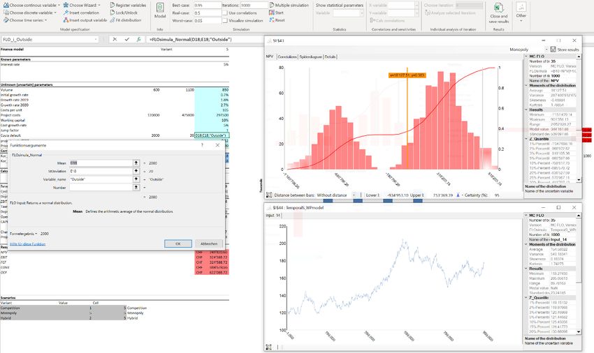
MC FLO User guide      1

Summary
MC FLO allows you to simulate uncertain events with the popular Monte-Carlo simulation
approach using Microsoft Excel®. Arrange easily variables
to a distribution or time series function and create
graphically correlations between them. During the Monte
Carlo simulation and at each iteration every variable is
assigned an allowable random value and the
corresponding results are stored. Analyse the results
using standardized charts, upload individual iterations
into the model and share the results considering different
scenarios – all this in the native Excel environment. No
separate viewers or other add-ins are required.

Monte Carlo simulations make decisions easier. Whether
in the launch of a product, in the context of corporate
planning, project controlling, the management of the
portfolio, risk identification and more... reveal how likely
the results will arrive and where you should pay attention
for success. With MC FLO you can judge which impacts can be accepted and which should be
avoided to ensure the best possible decision under uncertainty.

Use additionally the integrated forecasting tools to automatically predict potential future
developments (costs, revenues, etc.).

MC FLO is fully integrated into Microsoft Excel®. Call the integrated MC FLO functions easily as
any other functions are called in Microsoft Excel®. Familiarize yourself right away with MC FLO –
low incorporation costs, maximum efficiency! Use MC FLO to make data-oriented decisions.

                                                                             MC FLO User guide
                                                                          support@mcflosim.ch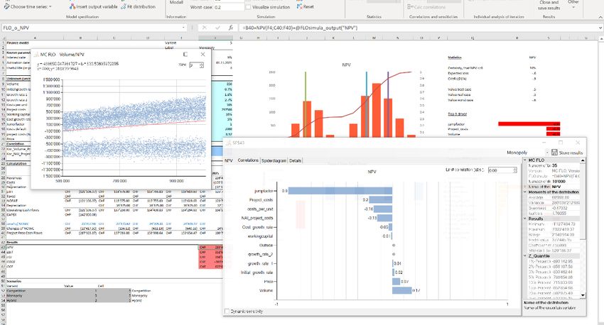
MC FLO User guide    2

SUMMARY                                                                 1

INTRODUCTION                                                            3

System                                                                  3

Installation                                                            3

More                                                                    3

Disclaimer                                                              3

PROCEDURES TO RUN A SIMULATION                                          4
  Model definition                                                      4
  Identification of uncertainty                                         5
  Fit distributions and time series                                    11
  Define correlations between inputs                                   14
  Insert the desired output variable                                   15
  Tips and Tricks                                                      15
  Input validation                                                     16
  Definition of scenarios and simulation mode                          16
  Starting the simulation and examining the results                    17
  Tools                                                                28
  Making predictions using time-series                                 35
  Frequently Asked Questions                                           36

SPECIFICATION OF MC FLO                                                38

LICENSE AGREEMENT                                                      39

                                                         MC FLO User guide
                                                      support@mcflosim.ch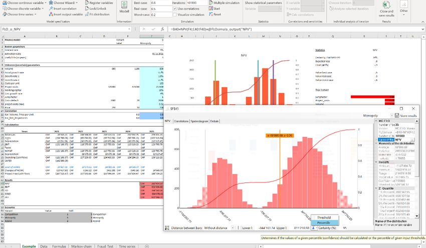
MC FLO User guide      3

Introduction
Welcome to MC FLO. MC FLO is a Microsoft Excel add-in simulation tool for Windows that puts
you in the position to calculate and visualize the uncertain future states and thus enables you to
make right decisions considering opportunities and drawbacks.

System
The simulation with MC FLO requires the installation of Microsoft Excel from at least version 2010.
MC FLO runs both on both 32-bit and 64-bit Excel systems. In addition to Excel, you need the .Net
runtime version 4.0, which can be obtained free of charge from Microsoft. For time restricted
licenses an internet connection is necessary to run the simulations. That's all.

Installation
MC FLO doesn’t need a specific installation. Unzip the desired version (32-bit or 64-bit) on any
local folder and copy the license file (MC FLO.txt) to your “My documents” folder. Then simply
click on the MC_FLO_FIRST.xll file and confirm the load procedure. Excel will start automatically
with a new ribbon menu called "MC FLO". You can immediately start with the specification of the
model with a new or already existing workbook. Info: If you want to start MC FLO automatically
with each Excel start, unpack the corresponding .zip file directly in the add-in directory of the
corresponding folder, like “C:\Users\your username \AppData\Roaming\Microsoft\AddIns” (the
path may differ, see Excel-> File-> Options-> Add-ins-> Go -> Browse the path of your add-in
folder)

Important: You must have previously stored the license key in your personal Windows document
folder. At https://www.mcflosim.ch/en/the-product/faq/ you can use a small program to
determine the document folder of your computer.

More
If after reading this manual some questions remain unanswered, do not hesitate to contact us
(mailto:support@mcflosim.ch). More information and educational videos are available at our
homepage. See also our blog contributions there.

Disclaimer
The program is designed and developed with the utmost care. However, since dependencies to
Microsoft Excel exist, a continuous functional test hasn´t be carried out. Nevertheless, by
exporting the entire data you have the model results always under control and therefore

                                                                               MC FLO User guide
                                                                            support@mcflosim.ch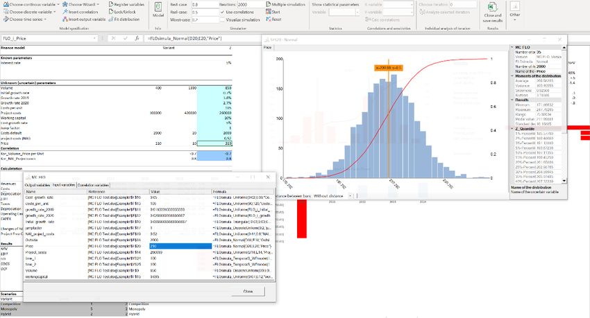
MC FLO User guide      4

maximum transparency. Please note that the manual may be subject to change at any time. The
images may differ from the actual program.

The respective rights of use of the names used here is governed by their holders.

Procedures to run a simulation
The simulation is performed in three steps

    a) Design a model and determine which variables are uncertain. Uncertain means that you
       do not know exactly which value may occur in the future. But you have some idea of the
       possible values.
    b) Assign each uncertain variable to a proper distribution or time series function and define
       dependencies (correlations) between these variables.
    c) Determine which calculated values you want to analyse additionally and start the
       simulation.

Model definition
The key-aspect of a simulation is the appropriate specification of a model that best describes the
situation to be examined. Evaluating a business case needs assumptions about the future
revenues and service costs incurred. Some assumptions may be given or a certain (prices), other
may be considered uncertain (penetration rate, costs of production). Additionally, dependencies

between the different variables must be considered. So, it may be that the unit cost of production
and the sales volume is negatively correlated. An increase in the sales volumes will therefore be
linked with a reduction in unit costs.

                                                                              MC FLO User guide
                                                                           support@mcflosim.ch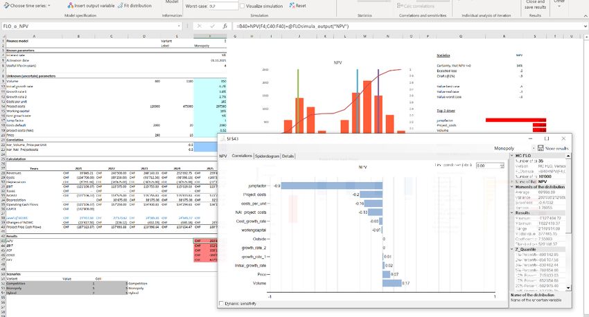
MC FLO User guide      5

Document the assumptions. Follow the rule of thumb that a poorly specified model will not be
salvaged by an extensive simulation run. Loosely speaking: A model to predict the weather will
not be suitable to evaluate a business opportunity.

Identification of uncertainty
After the model set-up, the uncertain variables must be assigned to a distribution, a function
which best reflect the future state of those variables. Here MC FLO show its glance. Specify which

model variable (or driver) should be defined as uncertain and hence to be “modelled”.

After selecting a distribution function using the ribbon fields an Excel dialog appears, where – as
with any other Excel-functions – different parameters must be inserted, whereby absolute values
or reference to other cells for
number related variables are
supported.       Note      that
characters that are not
compatible with the name
manager are replaced by a
«_» for the variable name.
After the insert process the
Excel cell will display the
expected value for the
selected           distribution
function.

                                                                               MC FLO User guide
                                                                            support@mcflosim.ch
MC FLO User guide      6

If you are not sure which function you should use, use the graphical wizard to display the functions
defined in MC FLO and then import them into Excel. Proceed as follows: go to "Choose Wizard"
and select from the various functions the one closest to your expectations. Enter the values
specific to the function under “Parameters”. Under "Number of Iterations", enter the number of
values to be considered in the simulation and define the number of columns to appear in the

diagram under "Number of bins". After pressing "Show", the result of the function (in the above
example the triangular distribution is shown) appears after a short time. Several quantiles are
displayed alongside the mean value, the minimum, maximum, variance and standard deviation.
In the chart a vertical line (“magic stripe”) will also been shown which displays the x-values of the
distribution and the corresponding quantile values. Just press the left key of the mouse over the
stripe and move to the right or to the left and the x and quantile values will automatically be
updated. By clicking the right mouse on the canvas, MC FLO loads the empirical data – if any - that
has been selected previously in Excel. The historical data will be loaded as "Real-Data" and shown
as a line graph. Please note that you will have to reload the historical data every time you choose
another distribution function. Enter a name under "Name of distribution" for the function, select
an appropriate cell in your model, and after pressing "Save" the function is inserted automatically
to the currently selected Excel cell.

Tip: Zoom-in or out the wizard window if the values of the magic stripe are not visible.

In Excel, the variable is presented both as a formula, starting with "FLO_i_", as well as a number,
which is defined as the average value of the defined limits. The cell is also marked with a
background colour and registered in the name manager of Excel.

                                                                                MC FLO User guide
                                                                             support@mcflosim.ch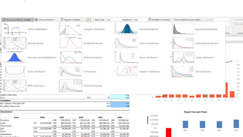
MC FLO User guide       7

Important: Each variable is stored in Excel in the name manager. This requires that the name of
the variable cannot contain empty spaces. Make sure that other variables that are not defined by
MC FLO, do not start with "FLO_i_”.

You can - like any other function in Excel - adjust the formula in the Excel editor to suit your needs.
The combination of several MC FLO functions is fully supported - use the variety and flexibility of
Excel! Note, however, that only MC FLO formulas are allowed in an individual cell as the principal
function. Otherwise, incorrect values will be shown in the result workbook. As highlighted in the
figure, only a MC FLO formula is inserted in a cell. You can use other Excel functions within a MC
FLO function, like “=FLOsimula_DiscreteUniform(if(E4
MC FLO User guide      8

In addition to the continuous distribution functions, discrete distributions are available. These are
then particularly useful if yes / no conditions are necessary or if only integer numbers should
appear in the model.

Info: In the discrete uniform distribution with the value range [0,1], the value 0 is shown as
standard in Excel.

Additionally, you can set the number of occurrences per iteration run for each function. This is
particularly useful when you want to multiply an uncertain variable with another variable
(constant or uncertain). For example, you can model the uncertain variable "revenue per

customer" and "number of customers" independently of each other and thus aggregate the total
                                                                         MC FLO User guide
                                                                      support@mcflosim.ch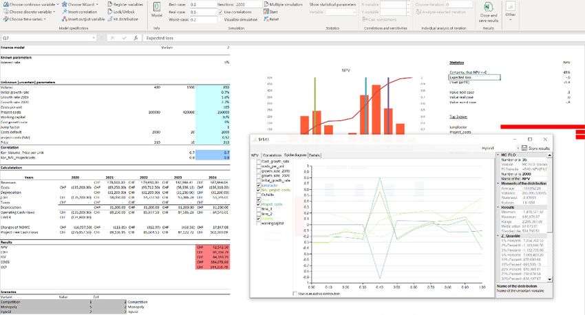
MC FLO User guide       9

to the desired "sales" figures. Commonly this is known as a compound function and can be
expressed in MC FLO with the optional “Number” parameter. In the illustrative example above
the compound functionality is accomplished by a triangle distribution for the revenue per
customer and a PERT distribution for the number of customers (which will be rounded
automatically in MC FLO to the nearest integer value). You can also correlate the uncertain
“Number” parameter with other uncertain functions of MC FLO, as expressed in a correlation
between the number of customers and the weather conditions in the mentioned example.

In addition to distributions of events, you can also select certain time series to model price or

volume developments.

MC FLO supports stationary auto-regressive models in form of AR(1), MA(1), ARMA(1,1),
additionally the Wiener process (also called geometric Brownian motion) with drift as a random
walk process with normal log returns and constant volatility and the ARCH(1) process for non-
constant volatility. Please note that for time series the magical stripe is not available. Please note,
that a simulation with thousands of iterations for a particular time series variable is equivalent to
the determination of one path of a time series process over thousands of periods. However, if you
like to simulate a time series process over the next 10 periods, you should enter 10 in the optional
“Number” parameter.

For continuous and discrete random variables, you can use the wizard to create a custom
distribution. There are two options available for this purpose. The first option consists to mark
the corresponding values of the model workbook and to transpose these into a histogram. After
                                                                                  MC FLO User guide
                                                                               support@mcflosim.ch
MC FLO User guide 10
pressing "Wizard" and "Custom defined", the data will be loaded into the wizard and you can
adjust the histogram with changing the "Number of bins". The second way is to directly import a
histogram, using following the six columns as a template. "Min" and "Max" indicate the
boundaries of the individual columns, "Number" the number of hits and "Percent" the relative
hits. The terms ending with "cum" represent accumulated values. Here is an example where eight
values are mapped into a histogram using 12 rows.
Min Max Number Number cum. Percent Percent cum.
266347 296025 1 1 0.125 0.125
296025 325703 0 1 0 0.125
325703 355381 0 1 0 0.125
355381 385059 2 3 0.25 0.375
385059 414736 1 4 0.125 0.5
414736 444414 0 4 0 0.5
444414 474092 1 5 0.125 0.625
474092 503770 1 6 0.125 0.75
503770 533448 0 6 0 0.75
533448 563126 1 7 0.125 0.875
563126 592804 0 7 0 0.875
592804 622481 1 8 0.125 1
(the last three columns are optional)
Note that a custom histogram should be loaded without headings. «Save» saves the user-defined
distribution in the model workbook, where the formula = FLOsimula_UserDefined («Data area»,
«Number of columns», «Name») is stored in the target cell.
Tip: If you only want to read values distributed over a row or a column, you can prefix a name in
the first cell, which is then used automatically as the name of the series when you open the
graphic wizard.
MC FLO User guide
support@mcflosim.chMC FLO User guide 11
Fit distributions and time series
Occasionally important historical data is presented in large quantities (such as data on the useful
life of plants) and not allocated to any distribution function due to a lack of expertise or other
factors. If the historical data is needed for the model, a suitable distribution function is to be found
as a first step. We have already introduced the graphical wizard. This presupposes, however, a
certain fundamental understanding. Another possibility is to be found under "Fit distribution".
Again, the data must be in an Excel. Mark the data and then go to "Fit distribution". Enter the
maximum value for “Degree of freedom”.
Often it is enough to set the value to 1 and to keep "increment" at 0.1. After pressing "Start fitting
data", all the continuous functions implemented in MC FLO are compared with the historical data
and the preferred outcome is the distribution which – in combination with the Kolmogórov-
Smirnov test - has the least squared deviation from the historical data.
For the historical data, the mean (average), minimum (min), maximum (max), variance (variance),
range, modal value and standard deviation (SDeviation) are displayed on the right above the
quantiles (or percentiles). The selected number of historical data is indicated as "Number of
iterations". Additionally, a new window, called “AIC” will be opened displaying the Akaide
Information criterion for all the continuous distributions (AIC = 2 * Number of parameter +
Number of iterations * ln(RSS)), where RSS is the residual sum of squares (on distributions, which
need the minimum and/or the maximum, the corresponding parameters are considered with a
value of 1.1 for each one). Now change to the model worksheet and the formula is automatically
transferred using the "Insert formula into current cell". Please note, that only continuous
distributions are fitted.
MC FLO User guide
support@mcflosim.chMC FLO User guide 12
Tip: If only after a substantial change of the parameters a new distribution is proposed, it is
recommended to use the previous distribution to prevent an “overfitting”. Note that in the result
window and in the AIC window MC FLO displays the “residual sum of squared errors”, by which
you can judge if the improvement is acceptable (as MC FLO uses the least squared approach, the
RSS should be minimized).
You can simulate every formula listed in the AIC window. Simply mark the formula, whereupon it
will be displayed in the main window.
Info: In some cases, it may be useful that you must weight larger deviations more strongly than
others. This is the case, if you need to estimate insurance damages. Activate the option "Prefer
higher values than lower ones" and enter the amount from which the higher weighting is to take
place in the text field that is displayed. In this case, MC FLO uses the beta distribution and
proposes corresponding values.
If you like to fit time series, select the "Fit time series" field und enter the number of forecast
data. Thus, the selected data is compared with the processes AR(1), MA(1), ARMA(1,1) - with
constant volatility - or with the ARCH (1) process - when there is no constant volatility. MC FLO
uses also the Wiener process “Geometric Brownian motion“ as measurement. In this case the
precondition of stationarity for the arithmetic mean is not necessary. For stationary time series
processes (AR, MA, ARMA) the AIC formula AIC = Log (variance) + (2 * Number of parameters /
Number of iterations) is used. In this case also Theil’s U is displayed. A good fit should produce a
U below 1. Please note that calculations may take some time depending on the number of
historical data and their distribution. We also recommend to visually compare the fitted function
generated by MC FLO with the historical data. Especially in the case, that the value generated for
MC FLO User guide
support@mcflosim.chMC FLO User guide 13
the "U-Test" is greater than one. In this case, the data has not passed the test for normal
distribution ("Anderson-Darling Test"), even though they may be normal distributed.
You can simulate every formula listed in the AIC window. Simply mark the formula, whereupon it
will be displayed in the main window and by pressing on "Simulate" MC FLO will initiate a new
time path. The upper and lower bound of this time path as well as the 50% percentile of the
forecast interval (95% confidence in 1,000 iterations) are displayed.
Tip: If you like to import another distribution that MC FLO has provided as the best solution, you
can do so following these steps: Copy the desired formula from the AIC window (pressing Ctrl+c)
and then insert it (pressing Ctrl-v) under “Result” in the “Fit distribution” window. Alternately you
can also copy all the results to the clipboard by marking first all cells of the AIC windows with
Ctrl+a and after clicking the menu bar on the AIC window all entries will be copied with Ctrl+c.
In addition to the stochastic time series processes, the result of the most appropriate Holt-Winter
model (additive or multiplicative) will be displayed. Note that the Holt-Winters models can`t be
used as variables in a simulation. On the other hand, with MC FLO you can create predictions
based on these models and perform automated predictions in Excel (see also Tools).
Determination of scenarios / option of multiple simulation
In some cases, you may want to investigate several options. Instead of creating your own model
for each option / variant, you can perform multiple simulations in MC FLO. To do this, select the
option and the corresponding parameters according to the following logic and by pressing on
«Multiple simulation» the selected rows will be registered for a multiple simulation:
Variant Value Reference
Competition 1 =F1
Monopoly 5 =F1
Under «Variant» enter a unique name for the variant / option. Under "Value" assign a unique
value (integer). The selection is completed with the cell reference (cell), which refers to the
selected option. The cells are highlighted with a gray background. Details can be found in the
example model supplied with MC FLO. Note that the selection of the variants has to be done
without the headings. If you want to reset the option of the multiple simulation, mark any empty
cell in the model and by pressing «Multiple Simulation» again the selection will be canceled. Info:
When the model is closed, the selection of the multiple simulation is automatically reset.
Therefore, confirm the saving of the model, so that the background color of the marked cells can
be reset. Note that the example file shipped with MC FLO uses this option.
MC FLO User guide
support@mcflosim.chMC FLO User guide 14
Define correlations between inputs
The definition of the input variables is the first important step. Next you specify dependencies
(correlations) and their intensity selecting "Insert correlation" in the menu bar. A new window
appears, from which you can select graphically the two input variables. Under "Correlation
coefficient" a possible value between (-1,1) must be selected. After confirmation by OK a new
formula is inserted in the called cell and highlighted. A variable starting with “FLO_c_” will be
registered.
You can choose between elliptical correlation relationships (normal, student-t [with 4 degrees of
freedom], archimedic copulas ([r-]Clayton, [r-]Gumbel, where r stands for the different rotations)
and, as a special case, non-symmetric correlations (asy. Gumbel, asy. Triangular and asy. Fréchet).
The correlation type is stored as an integer between 0 and 7 in the correlation formula. Note that
for some correlation relationships, Kendal’s Tau is used as an approximation. Under the entered
correlation coefficient, the resulting rank correlation coefficient appears in grey colour.
Info: The correlations are computed only during the simulation. Therefore, the variables are not
updated after the correlation has been defined. Please note that for time series the correlation is
based on the random component. Therefore, a correlation between two time series process can
only be modelled if the variables behave time-invariant at each iteration. You can´t correlate time
series where the parameter “Number” is greater than 1.
Info: Archimedean copulas can only be defined in MC FLO as a bivariate relationship. For example,
you define an Archimedean correlation between "quantity" and variable "x". Consequently, it is
not allowed to define a further correlation for either "quantity" or "x". Note that the definition of
MC FLO User guide
support@mcflosim.chMC FLO User guide 15
an Archimedean correlation relationship (copula) means that all correlations in the model must
be of type bivariate.
Correlation relationships of continuous and discrete distributions in the range of the 5% and 95%
quantiles are highlighted in green and red colour. Also note that only 1'000 records are displayed
in the window.
Entering the correlations concludes the modelling part. By linking the uncertain variables and
parameters defined as safe, you can represent the desired result.
Insert the desired output variable
As the last step and for evaluation/analysing purposes output variables, that contain the result of
the calculation (ex. net present value), must be defined.
With confirmation of the "Insert output variable" button, you are prompted to enter a name. Pay
attention to the conditions applicable to the input variable name conventions. After the name
specification is finished a formula called "= + FLOsimula_output ("variable name")" is inserted and
the target cell highlighted. A variable starting with "FLO_o_" will also be registered in the name
manager of Excel. Before the "+" in the formula the reference to the cell which is to be analysed
has to be inserted.
By entering at least one input variable and one output variable the model specification is formally
completed and you can start the simulation.
Tips and Tricks
Very often it can happen that you want to assign the input, correlation and output variables
continuously in a column or row. Instead to call the input mask or the wizard for each cell
individually, you can
proceed as follows: Go into
the cell which will contain
the variable and enter the
formula by hand. Start with
"=FLOsimu”. The functions
defined in MC FLO will
appear. Choose the right
one which you want to
include. Take as the
variable name a reference
to another cell. Confirm
the entry for all
parameters. Then tighten
the definition to the range which should be filled with the new variables. Please note that for
MC FLO User guide
support@mcflosim.chMC FLO User guide 16
compatibility reasons the parameter “Number” cannot be passed as a parameter. You must
introduce the number of occurrences after the automatic processes has been finished.
Close the manual entry with "Register variables". As a result, the variables will be registered in
MC FLO.
For constant and discrete distribution you can define barriers with the distribution function
«FLOsimula_Bounded». This function must be entered manually using the Excel editor and then
completed by confirming with "Register variables". The function «FLOsimula_Bounded
(Reference, LowerLimit; UpperLimit)» contains as first argument the MC FLO variable which has
to be bounded, the parameters «LowerLimit» give the lower barrier and «UpperLimit» the upper
barrier.
Input validation
Check the selected parameters by calling the appropriate "Show" button. You will see a summary
of all the variables in the selected category (Input, correlations, Output). The affected cell is
highlighted in Excel by clicking on a column of the summary. Info: If the preview mode is enabled,
the distribution and correlations will be displayed graphically. This will also be possible after a
simulation run (see below).
Important: If you do make changes during or after completion of the model, take note of the
variables involved and remember the referenced values. If you want to delete an input variable
that is referenced by another input variable, change the specification of the last one before the
former is deleted.
You can fix individual variables to the initial value as required. This keeps the variables unchanged
for each iteration. To do this, select the input variable to be fixed and confirm the selection with
«Lock/Unlock». The selected input variable is highlighted in red. During the simulation, the locked
variables remain unchanged with the expected value of the distribution. The fixation is cancelled
by selecting the variables again and pressing "Lock/Unlock". Make sure that the input variables
are red-coloured only having used the MC FLO “Lock/Unlock” function, otherwise they will be
blocked.
Definition of scenarios and simulation mode
MC FLO supports the definition for three scenarios ("worst", "real" and "best"). For each one you
must specify the
required confidence
level or quantile. The
confidence defines
the region in which
the required quality
is very likely to
happen. Example:
MC FLO User guide
support@mcflosim.chMC FLO User guide 17
You plan the investment budget for the next year. Values between 10,000 and 80,000 may result
from the simulation. Which value should be considered in the budget? You define in advance for
the real case that with a “probability” of 10% a budget overrun can be tolerated. In the worst
case, you want to allow enough funds in the budget, so that a budget overrun occurs only with a
5% “probability”. For the real case, you define a confidence level of 0.9 (1 minus "residual
probability") and for the worst case the 0.95 quantile is defined. After the simulation run the
corresponding value for each scenario is displayed in the result workbook.
You can define in advance how Excel will behave in each iteration. By checking "Visualize
simulation" the values of the input, the outputs and the embedded Excel charts are actualized at
each iteration. Note that this simulation mode is very slowly and should be used only for
demonstration purposes.
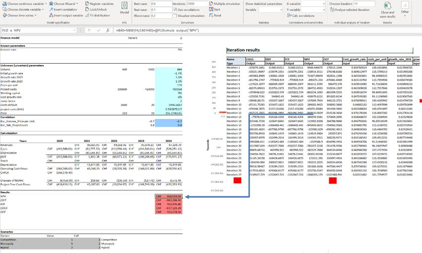
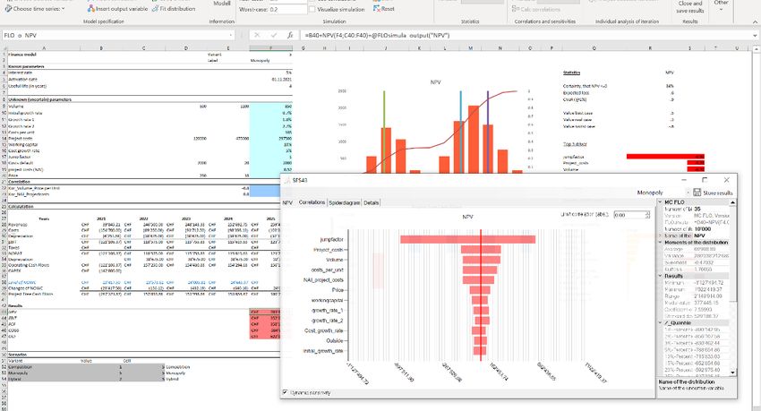
Starting the simulation and examining the results
Now is time to start the simulation. Select an output variable, specify the number of iterations at
"# iterations" and start the simulation with "Start". On the status bar of Excel, the progress of the
calculation is displayed. The end of the calculations will be completed with the appearance of a
separate window containing the results from the selected output variable. As with the wizard
interface you can also use the magic stripe to display the x-values of the resulting distribution and
the corresponding quantiles. Press the left mouse button on the magic stripe and move it to the
right or to the left and the corresponding values will be displayed automatically.
In the lower range, the values for the 95% confidence level (security) appear, also the
corresponding bars appears in highlighted color. You can adjust the level or under by selecting
"Thresholds" determine new lower (Lower l.) and upper (Upper L.) boundaries and the associated
confidence level (see also https://youtu.be/ZcpmDhRs33I).
Resize the window if necessary in order to view the values on your screen. From the resulting
output window you can store the entire results in a separate workbook by pressing “Store
Results”.
By adjusting the number of columns in the window or by changing the color or the number of bins
you can adjust the histogram for your purposes. For output variables you can additionally use a
tornado graph to display the correlations (according to Pearson) between the selected output
variable and all input variables. This allows you to quickly identify the crucial input variables and
thus to make better decisions. However, please note that the Pearson correlation coefficient
asumes a linear relationsship.
MC FLO User guide
support@mcflosim.chMC FLO User guide 18
Navigate through each input, correlation or output variable after a simulation run and at each
time a new window appears, summarizing the outcome with standard statistics. Input variables
are shown in blue, output variables in orange colour.
MC FLO User guide
support@mcflosim.chMC FLO User guide 19
By pressing any of the correlation bars a new window will open, which will show the details in a
chart. This will give you a visual check if Pearson's linear correlation is feasible, showing the linear
regression equation. In addition, you can also see the effects using a dynamic sensitivity.
In this case the minimum and maximum of an interval based relationship between the input
(where the input variable is initially sorted in ascending order) and the output variable is shown.
MC FLO User guide
support@mcflosim.chMC FLO User guide 20
As a complement MC FLO facilitates through a spider diagram the correlations by quantile, either
in isolation or cumulatively. At the outset, the input variables that have a correlation equal to or
greater than +/- 0.3 in any of the quants will be highlighted in any of the quants. In the example
above the correlation between the variable "jumfactor" and "NPV" is zero in the quantile between
0 and 0.1, comprising corresponding Values of the NPV between -1'048M and -748k.
MC FLO User guide
support@mcflosim.chMC FLO User guide 21
If you use the "Use cumulative distribution" option instead, the correlation will be displayed
cumulatively (the "jumpfactor" variable has a correlation of approximately -0.9 between the NPV
minimum (-1'048M) and quantile 0.4 (equivalent to 140k). In quantile 1 the cumulative correlation
is equivalent to the calculated correlation.
Note that you can´t use a cell in which a correlation relationship has been defined as the source
cell for a simulation. Go to a cell with an output variable or to an empty cell before starting the
simulation.
If you have activated the multiple simulation, you can make a graphical comparison between the
variants under "Details" for the selected output variable. You can also select the individual
variants of the corresponding variables in the main window, which triggers Excel to refresh the
cells and graphics.
MC FLO User guide
support@mcflosim.chMC FLO User guide 22
In addition you can select several input and/or input variables at once and display the
corresponding values in a summary window, optionally adjusting the confidence level. Please note
that only 1’000 variables can be displayed at once.
MC FLO User guide
support@mcflosim.chMC FLO User guide 23
Info: To minimize the calculation time no further action with Excel is possible after starting the
calculations.
In order to simplify the exchange with users who do not want to have MC FLO installed, you have
the option to store the input variables, correlations and the results as a background image in the
corresponding cell as a comment. By double-clicking on the corresponding diagramm, the window
is saved in the corresponding cell. Note, however, that existing comments will be overwritten.
Info: You can reset the simulation with “Reset”. In this case all the results from the simulation will
be erased from the computer memory.
Tip: To validate the model we recommend starting the simulation with a small number of
iterations. From the results displayed, you determine whether the model needs to be adjusted
before a exhaustive simulation (with thousands of iterations) should be performed.
MC FLO User guide
support@mcflosim.chMC FLO User guide 24
Tip: You can visualize the input, the correlations and output variables in a preview simulation
mode before the first simulation run. Proceed as follows: Under «Other -> “Seed» parameter
enter a -1. Then go to a cell with an input, correlation or output variable and a new window will
open which shows the shape of the variable according to the formula definition. You can leave
the preview simulation mode by assigning the seed variable a value different to -1. Note that the
preview simulation mode is not faster than the normal simulation mode and uses only random
variables for the input and correlation variables. Note that a preview simulation mode is pre-build
for the input variables without the need to set the seed parameter. For this select a cell containing
a input variable and press “Start”. A new window with the possible results will be shown.
As mentioned before, the results can be stored by pressing “Store results” from the corresponding
window of an output variable after a simulation run. The results will then be displayed in a new
workbook, called the result workbook. This workbook will initially contain the following
worksheets
● Data: Here all the values of the input variables and the output variables of each iteration
are stored. You can verify the results with reference to the numbers stored.
Info: The data in the worksheet "Data" is write-protected.
● Summary: All the input and output variables with the calculated maximum, minimum and
average is value are displayed, followed by the corresponding variance, standard
deviation and the results of the scenarios ("worst", "real" and "best"). The information is
always compiled with the information stored on the Worksheet “Data”.
MC FLO User guide
support@mcflosim.chMC FLO User guide 25
Additionally, the skewness, kurtosis and all quantiles are represented in 5%-point steps,
the extreme values (in 1%-point steps) and the +/- 3%-point deviations from the real case
are displayed.
● Statistics: According to the selected input or output variable from the result workbook
the parameters of the summary worksheet are shown. Additionally, a confidence level of
the mean (the standard is set with a confidence level of 0.9), a histogram with the best
and worst scenario outlined by a vertical line, the limit value (typically the zero value) and
a cumulative distribution curve is shown. The mentioned tornado graph reveals the
relationship (correlation) between the selected variable and all other variables. Info: The
Excel formula to determine the confidence level of the mean assumes a normal
distribution. If the examined variable does not follow a normal distribution, the calculated
confidence level of the mean is not meaningful and should not be used further.
You can freely select the number of bars ("classes") to be displayed in the histogram. From the
result workbook enter the number in the corresponding field “Set bins” and confirm with «Change
histogram». Note that MC FLO sets the number of bars back to their original value each time a
new result workbook is opened.
Info: To analyse time series and their respective correlations you should copy the data from the
sheet “data” to a new sheet and insert a new diagram if necessary. You can now easily check the
correlations visually between the data. Please note that the correlation may differ from the
MC FLO User guide
support@mcflosim.chMC FLO User guide 26
correlations defined in the model (“Spearmans Rho”). This corresponds to the fact, that
correlations between time series are established upon the noise process.
Tip: You can change the label of the axes individually. The diagram can be integrated into other
Microsoft Office products or you can share the spreadsheets with others. Change the colours, the
size, add new information and so on. No additionally viewers are needed!
The close of the new workbook is completed with "Close and save results". The workbook is saved
in the same folder where the model is stored. It can always be opened and analysed by MC FLO
again.
Info: The new workbook is always saved with the date (day, month, year), the time (hour, minute,
second), separated by "_" each, and the label "MC_FLO.xls" additionally to the name of the model
specified. Info: if you have performed a simulation with more than one million iterations than only
the iteration results will be stored in a “csv” file.
In addition to the analysis of individual variables, you can under "Correlation and sensitivities"
examine the relationship between two variables, both graphically and numerically by regression
analysis. Under the "X-variable" and from the result workbook ribbon fields you select the
(independent) first variable and under "Y-variable" a (dependent) second variable. Confirm the
selection with "Calc correlations". In the result workbook a new sheet with the label "Sensitivity"
is inserted and displayed. In the left side the correlations of all variables with respect to the
selected "Y-variable" are shown. In the middle the simple linear regression analysis of the two
selected variables is displayed. By entering new values in cell I5 you can calculate a forecast using
simple linear regression. The corresponding approximated 95% forecast interval is presented in
MC FLO User guide
support@mcflosim.chMC FLO User guide 27
cells K5 and L5, with an approximation based on the normal distribution and assuming a large
sample (at least 300 iterations of a continuous or discrete distribution). Also note that the
residuals must be independent and normally distributed if you use a linear regression. From line
D52 you can read further statistical results of the regression analysis (hidden by default). You can
perform further predictions using the linear regression analysis. Enter in cell I4 a new value for
the independent variable and on cell I5 the estimated value is shown.
For the dependent variable, the correlation with the independent variable is displayed graphically
in 10% -quantile steps. In this way, you immediately discover the area in which the correlation is
particularly pronounced. A linear regression equation indicates the direction.
At the right the tornado graph from the summary worksheet is shown.
Info: If you analyse two variables that were set with a correlation relationship before the
simulation run you will discover that the correlation result in Microsoft Excel does not coincide
with the entered correlation coefficient. This is due to the method of calculation of MC FLO. MC
FLO compiles the Spearman algorithm to determine the (rank-order) correlation coefficient,
however, Microsoft Excel uses the linear Pearson correlation coefficient.
MC FLO allows you to check the calculations individually. You can load the simulation results of
the uncertain variables in the original model and compare the resulting results in Excel with the
calculated data in the worksheet "Data". Choose under "Individual analysis of iteration " from the
model workbook the selected iteration and confirm the selection with "Analyse selected
iteration". As a result, the values of the input variables of the concerned iteration are loaded from
MC FLO User guide
support@mcflosim.chMC FLO User guide 28
the result workbook into the original model, where they appear as numbers rather than as a
formula. You can restore the formulas by closing the result workbook or by pressing any “Show”
ribbon button from the model workbook.
It is easy with MC FLO to share the result with others. All the data of the calculations and diagrams
are stored in native .xls files and can be analysed further with MC FLO. Independent advisors can
check and proof the values by other instruments. Be one step closer with MC FLO and your
success!
Tools
MC FLO also provides some functions via the formula editor of Excel or by the ribbon buttons
provided by MC FLO. Note that some functions require a previously performed simulation,
otherwise a value of -1 is displayed in the cell. In addition, we recommend that you do not use
these functions in a visual simulation. Some functions can also be evaluated with reference to
variants (multiple simulation) or using a visual simulation. To combine a visual simulation with a
live creation of a histogram, we refer to the Excel program enclosed with MC FLO.
Formulas
fmc_Name(Name): Returns the name of the unique MC FLO variable from the specified cell of the
same workbook; can be used in conjunction with other functions, like
fMC_Min(fMC_Name(Name)).
fMC_Spider (Name1; Name2; Value1; Value2): Calculates the linear correlation coefficient
(Pearson) between the data points Value1 and Value2 of the variable Name1 with the
corresponding data of the variable Name2.
fMC_ExtremeValue (Name1; Pos): Returns the value at the i-th position of the sorted list of the
variable Name1.
fMC_PosValue (Name1; Pos): Returns the value at the i-th position of the variable Name1.
fMC_Bayes (Name1; Comparison1; Value1; Name2; Comparison2; Value2): Calculates the
conditional probability for event A (Name1), given that event B (Name2) has arrived. Example:
fmc_Bayes('NPV';' >=';1000;' Project costs';' >=';100) calculates the probability that NPV is greater
(or equal) than 1000, given that the project costs are greater (or equal) than 100.
fMC_BayesV (Name1; Comparison1; Value1; Name2; Comparison2; Value2; Optional Percentile):
Calculates the average value induced by event A (Name1), given that event B (Name2) has
occurred; If percentile is given, then the percentile value of the result is taken into account.
Example: fmc_BayesV (‘NPV’; ’>=’; 1000; ’Project costs’; ’>=’; 100; 0.1) calculates the 10%
percentile value of NPV >= 1000, given that the project costs are over 100. If Percentile is not
specified, the average value of NPV above 1000 is calculated.
MC FLO User guide
support@mcflosim.chMC FLO User guide 29
fMC_FitC (column1; column2): Performs a correlation adjustment of two series located in
column1 and column2. The result is the adjusted correlation type as a number between 0 and 7
(see also Define correlations between inputs).
fMC_Pearson (column1, column2): Determines the correlation coefficient according to Pearson
of two rows of data, which are in column1 and column2.
fMC_Spear (column1, column2): Determines the rank correlation coefficient according to
Spearman of two rows of data, which are in column1 and column2.
fMC_Sort (column1, pos, [optional] Sort = 0,1): Returns the position (pos) of a sorted list whose
numbers are displayed in a column. Sort is used to specify whether the list is sorted ascending (0,
defined as default) or descending (1).
fMC_BSMVal(Basis, Time, Interest, Sigma): Returns the price of an underlying after “Time”
periods, given the “Basis” price, a riskless interest rate “Interest” and a constant volatility “Sigma”
according to the Black-Scholes-Merton” model.
fMC_Batch_Time (Matrix1, Number, ResultOrder, Selection, NumIterations, Percentil): Marks the
column or row selected in Matrix1 as time series for a batch run. "Number" defines the number
of data to be forecast, "ResultOrder" determines how the estimated historical and the forecast
data should be displayed in Excel (0 = line by line, 1 = column by column), with the forecast
function selected based on the "Selection" criterion (0 = Akaide Information Criterion, 1 = Sum of
Residuals). “NumIterations” reflects the number of iterations and “Percentil” the resulting
percentile to be considered.
fMC_Batch_HW_D_Time (Matrix1, Number, ResultOrder, Selection, NumIterations, Percentil):
Marks the column or row selected under Matrix1 as a time series for a batch run using the Holt-
Winters models (additive, multiplicative), with the data on a daily basis and a forecast for the next
few days. "Number" defines the number of forecast data, "ResultOrder" determines how the
estimated historical and new forecast data should be displayed (0 = line by line, 1 = column by
column), with the forecast function selected based on the "Selection" criterion (0 = Akaide
information criterion, 1 = sum of the residual squares). "NumIterations" defines the number of
iterations and "Percentil" the percentile. With a "percentile" of 0.5, the standard forecast is
performed.
fMC_Batch_HW_M_Time (Matrix1, Number, ResultOrder, Selection, NumIterations, Percentil):
Marks the column or row selected under Matrix1 as a time series for a batch run using the Holt-
Winters models (additive, multiplicative), with the data on a monthy basis and a forecast for the
next few months. "Number" defines the number of forecast data, "ResultOrder" determines how
the estimated historical and new forecast data should be displayed (0 = line by line, 1 = column
by column), with the forecast function selected based on the "Selection" criterion (0 = Akaide
information criterion, 1 = sum of the residual squares). "NumIterations" defines the number of
MC FLO User guide
support@mcflosim.chMC FLO User guide 30 iterations and "Percentil" the percentile. With a "percentile" of 0.5, the standard forecast is performed. fMC_Batch_HW_Q_Time (Matrix1, Number, ResultOrder, Selection, NumIterations, Percentil): Marks the column or row selected under Matrix1 as a time series for a batch run using the Holt- Winters models (additive, multiplicative), with the data on a quarterly basis and a forecast for the next few quarters. "Number" defines the number of forecast data, "ResultOrder" determines how the estimated historical and new forecast data should be displayed (0 = line by line, 1 = column by column), with the forecast function selected based on the "Selection" criterion (0 = Akaide information criterion, 1 = sum of the residual squares). "NumIterations" defines the number of iterations and "Percentil" the percentile. With a "percentile" of 0.5, the standard forecast is performed. fMC_BootStrap (Matrix1, NumIt, Confidence, Percentile): Selects the column or row selected under Matrix1 and determines the confidence interval of the mean of that sample using NumIt of new samples (sampling with replacement). Result is a string with (mean value, lower range, upper range). If “Percentile” is specified, the confidence interval will be calculated with regard to the corresponding percentile. fMC_BootStrapN(Name, NumIt, Confidence, Percentile): Selects the variable “Name” of a simulation and determines the confidence interval of the mean of that sample using NumIt of new samples (sampling with replacement). Result is a string with (mean value, lower range, upper range). If “Percentile” is specified, the confidence interval will be calculated with regard to the corresponding percentile. fMC_AD(Matrix1): Performs an Anderson-Darling test to check for normal distribution of the data selected under Matrix1. Returns True if the data is very likely to be normally distributed. fMC_AD(«Name»): Performs an Anderson-Darling test to check for normal distribution of the variable selected under “Name”. Returns True if the data is very likely to be normally distributed. fMC_Best(Optional Value): Returns the defined confidence level of the best case. If Value> = 0 and Value = 0 and Value = 0 and Value
MC FLO User guide      31

fMC_ExpGainV(«Name»): Returns the variance of the values above the expected gain of 0 from
the distribution “Name”.

fMC_ExpLoss(«Name»): "Returns the expected average of all values below the expected gain of 0
from the distribution “Name”.

fMC_ExpectedShortfall(«Name», «percentile»): Calculates the expected shortfall from the
distribution “Name” from the value-at-risk defined at “percentile”.

fMC_Percentile(«Name», «Percentile»): Returns the value at the k-percentile from the
distribution “Name”.

fMC_PercentileValue(«Name», «Value»): Returns the percentile for a given “value” from the
distribution “Name”.

fMC_PercentileInterval(«Name», «Lower_Limit», «Upper_Limit»): Returns the confidence level
(in %) from the distribution “Name”, conditional on a lower (“Lower_Limit”) and upper limit
(“Upper_Limit”).

fMC_CV(«Name»): Returns the coefficient of variation of the distribution “Name”.

fMC_Semivariance(«Name»): Returns the semivariance of the distribution “Name”.

fMC_Skewness(«Name»): Returns the skewness of the distribution “Name”.

fMC_Kurtosis(«Name»): Returns the kurtosis of the distribution “Name”.

fMC_StdS(«Name»): Returns the of sample tandard deviation the distribution “Name”.

fMC_Variance(«Name»): Returns the sample variance of the distribution “Name”.

fMC_Average(«Name») / fMC_Mean(«Name»): Returns the average of the distribution “Name”.

fMC_Min(«Name»): Returns the minimum of the distribution “Name”.

fMC_Max(«Name»): Returns the maximum of the distribution “Name”.

fMC_Sum(«Name»): Returns the sum of the distribution “Name”.

fMC_FinancialValue («Name1», «Name2», «Value2», «Diff», «Value1»): Calculates the value of
event A (Name1), given that event B (Name2) has occurred. For event B, the search area contains
+/-% of the limit entered under Diff. The result is the percentile value “Value1” of “Name1”.

fMC_FinancialDTrans (“Initial”, “Periods”, “ActualYear”, “Amount”): Determines the proportional
share per year (via “Actual Year”) of the value “Amount”, starting from “Initial” and “Periods” (in
year) time.

                                                                               MC FLO User guide
                                                                            support@mcflosim.ch
MC FLO User guide 32
fMC_Mode («Name», «UsedBins»): Determines the most frequent value of the «Name»
distribution on the basis of a histogram with the number of «UsedBins» columns.
fMC_ConditionPosValue («Name1», «Value»): Returns the position in the list of «Name1» which
corresponds to the specified value «Value».
fMC_RegressionX(«Name1», «Name2»): Calculates the linear regression slope of two variables.
Name1 is x-vector, Name2 is y-vector.
fMC_RegressionY(«Name1», «Name2»): Calculates the linear regression intercept of two
variables. Name1 is x-vector, Name2 is y-vector.
fMC_DSensitivity(«Name1», «Name2», «DSensotype», «NumberBins»): Returns the dynamic
sensitivity between two variables, whereby Name1 corresponds to the input and Name2
corresponds to the output variable. DSensotype indicates, which value should be returned; 0 =
range, 1 = minimum, 2 = maximum. NumberBins specifies the number of bin used to make the
calculation.
fMC_GetInputName(«Pos»): Returns the input variable at position Pos.
fMC_GetUserDefinedInputName(«Pos»): Returns the output variable at position Pos.
fMC_GetOuputName(«Pos»): Returns the user defined input variable at position Pos.
fMC_Bayes4(«NameX», «CompareX», «ValueX»…): Calculates the probability for event A
(Name1), given that event B, C, D to E (Name2, Name3, Name4, Name5) has occurred, see
fmc_Bayes.
fMC_Bayes4V («NameX», «CompareX», «ValueX»…, «Percentil»): Calculates the value induced by
event A (Name1), given that event B, C, D to E (Name2, Name3, Name4, Name5 ) has occured, see
fmc_BayesV.
fMC_Density («Name»,«Value»): Determines the density at the point 'Value'.
fMC_Bin («Value»): Specifies the number of columns in a histogram via "Value" (globally valid).
fMC_SimulaOn(«Value»): Workbook-Simulation modus: Determines whether random values
(TRUE) or the expected value of the distribution function (FALSE) should be displayed after the
worksheet / workbook has been recalculated. Note that the simulation results can only be
evaluated with the value FALSE.
Matrix-functions
fMC_PortfolioCombn(«AValue»): Calculates the number of portfolio combinations (without
repetition, without order requirements) of n (“AValue”) titles.
MC FLO User guide
support@mcflosim.chMC FLO User guide 33
fMC_PortfolioMatrix(«aMatrix», «AsInput», «Comparex», «Comparesx», «Comparevx»):
Determines the number of possible portfolios (matrix notation), where n titles are used. The result
is a n x 2 matrix, where the first column contains the MC FLO variables and the second one the
corresponding names of the portfolio. If AsInput is true (1), the variables are interpreted as input,
otherwise as output variables.
fMC_PortfolioManualMatrix («aMatrix», «cMatrix», «isInput»): Determines a portfolio based on
a 0-1 matrix. Objects with a 1 are added to the portfolio. AMatrix corresponds to the names of
the titles (as nx1 matrix) from which the portfolio is determined and cMatrix is an nxm matrix with
0-1 numbers. Make sure that the number of lines in the aMatrix matches the number of lines in
the cMatrix matrix. If isInput is true (1), the variables are interpreted as input, otherwise as output
variables.
fMC_PortfolioCorrMatrix((«aMatrix», «FillRandom»): Determines the correlation matrix of a
portfolio of n titles. Result is a q X 1 Matrix. If FillRandom is true (1), then every correlation
association is prebuild with a correlation coefficient between -0.3 and +0.3 (random number),
otherwise the correlation coefficient is 0.
fMC_PortfolioCorrMatrixF («aMatrix», «CorrelT»): Determines all correlation combinations and
their correlation coefficients from n variables of «aMatrix». The result is a matrix with n x (n-1) /
2 rows; «CorrelT»: Specifies the correlation coefficient: 0 = Pearson, otherwise Spearman.
fMC_SimpleMarkovChain(«aMatrix», «n»): Model of a Markov chain to predict the final state
after n periods, parting from a n x m matrix.
fMC_NBT(«aMatrix», «UseSummary»): Checks whether data is Newcomb-Benford distributed
using the Chi-squared test. Output is a 18x3 matrix, where the first 9 lines represent the
frequencies of the numbers 1 to 9 (column 1 = measured; column 2 = Newcomb-Benford
distribution).
fMC_LDT(«aMatrix», «UseSummary»): Checks whether the last digit before the decimal separator
is uniform distributed using the Chi-squared test. Output is a 19x3 matrix, where the first 10 lines
represent the frequencies of the numbers 0 to 9 (column 1 = measured; column 2 = Uniform
distribution).
fMC_BayesCombine (“NumberX”, “ShareX”, “ReturnData”, “NumBin”): Combines up to five
different priori probability distributions into an aggregated priori distribution. ReturnData:
Specifies whether the data of the combined distribution should be expressed directly as an nx1
matrix (TRUE) or as an nx3 histogram (FALSE). If as a histogram, the number of columns is used
via NumBin.
fMC_BayesMCMC ("Name1", "Name2", "BurnIn", "Thinning", "NumberIterations", "ReturnData",
"NumBin"): Combines the priori probability distribution (Name1) with new data of the same type
MC FLO User guide
support@mcflosim.chYou can also read