Symplectic Integration for Multivariate Dynamic Spline-Based Model of Deformable Linear Objects
←
→
Page content transcription
If your browser does not render page correctly, please read the page content below
Symplectic Integration for Multivariate Dynamic Spline-Based
                                                         Model of Deformable Linear Objects
arXiv:2108.08935v1 [cs.RO] 19 Aug 2021

                                                                      Alaa Khalifa* and Gianluca Palli
                                                      Department of Electrical, Electronic and Information Engineering,
                                                                        University of Bologna, Italy
                                                *On leave from Department of Industrial Electronics and Control Engineering,
                                                       Faculty of Electronic Engineering, Menoufia University, Egypt
                                                                 Email: alaa.khalifa@el-eng.menofia.edu.eg

                                         Abstract                                                     However, humans manipulate those objects naturally,
                                                                                                      with high dexterity, and without any particular issue.
                                         Deformable Linear Objects (DLOs) such as ropes, ca-          In facts, manipulating these deformable objects has a
                                         bles, and surgical sutures have a wide variety of uses       wide variety of uses in domestic facilities and health-
                                         in automotive engineering, surgery, and electrome-           care, such as robotic surgery [17], assistive dressing,
                                         chanical industries. Therefore, modeling of DLOs             garment sorting or folding clothing [25], [31]. More-
                                         as well as a computationally efficient way to pre-           over, it is involved in manufacturing, aerospace [35],
                                         dict the DLO behavior are of great importance, in            automotive, and electromechanical industries gener-
                                         particular to enable robotic manipulation of DLOs.           ally [18],[7].
                                         The main motivation of this work is to enable effi-
                                                                                                         On the contrary, the manipulation of deformable
                                         cient prediction of the DLO behavior during robotic
                                                                                                      objects is still a challenging activity for robots. This
                                         manipulation. In this paper, the DLO is modeled
                                                                                                      is the main reason why many assembly procedures
                                         by a multivariate dynamic spline, while a symplec-
                                                                                                      involving such deformable objects are still performed
                                         tic integration method is used to solve the model
                                                                                                      manually. One of the main reasons why robots have
                                         iteratively by interpolating the DLO shape during
                                                                                                      such limitations in deformable object manipulation
                                         the manipulation process. Comparisons between the
                                                                                                      is due to their complex behaviors, unpredictable ini-
                                         symplectic, Runge-Kutta and Zhai integrators are re-
                                                                                                      tial configuration, and limited capability in measur-
                                         ported. The presented results show the capabilities
                                                                                                      ing their state.
                                         of the symplectic integrator to overcome other in-
                                         tegration methods in predicting the DLO behavior.              A thoughtful survey can be found in [32] that fo-
                                         Moreover, the results obtained with different sets of        cuses on deformable object manipulation by robots
                                         model parameters integrated by means of the sym-             in industrial and domestic applications. Actually,
                                         plectic method are reported to show how they influ-          the dynamics of deformable objects is complex and
                                         ence the DLO behavior estimation.                            nonlinear. Therefore, the state estimation of a de-
                                                                                                      formable object is challenging, and the forward pre-
                                                                                                      diction is expensive. Robust and effective methods
                                         1    Introduction                                            to manipulate deformable objects and predict their
                                                                                                      behavior remain extremely difficult to build, despite
                                         Many of the objects we handle every day are highly           the several applications and attempts made by the
                                         deformable and with prevalent plastic behavior.              robotics community [32].

                                                                                                  1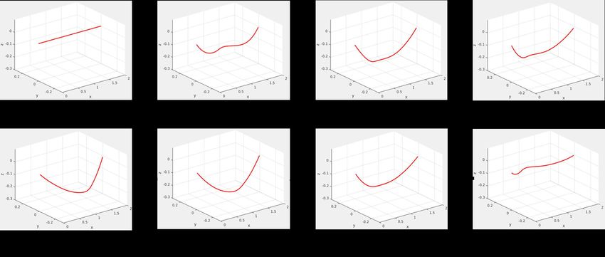
In this work, the numerical integration of De-               namic spline [38], Finite element [5], and other mod-
formable Linear Objects (DLOs), such as strings, ca-            els. The methodology, advantages and disadvantages
bles, electric wires, catheters, ropes, and so on, is ad-       of each model method are discussed in detail in [24].
dressed, since efficient solutions to this problem will         The dynamic spline is one of these methods which
enable the implementation of robotized solution in              provide a good theoretical basis, continuous model,
many relevant subfields of the large and diverse in-            higher authenticity. A geometrically reliable model
dustrial manufacturing. DLO manipulation is funda-              of DLOs is generated and adopted in [36] to execute
mental in automotive manufacturing, e.g. for wiring             numerical simulations on the motion of the object
harness preparation and electrical cable installation           under gravity and during environmental interaction.
inside the vehicle structure, as well as in medical             For interaction simulation, a linearized spline-based
surgery, e.g. in suturing in which a flexible wire in           DLO model named quasi dynamic splines is created
a straight configuration needs to go to a knot [26],            in [37].
and have a vital role in other fields such as architec-            Owing to the inherent trade-off between precision
ture and power distribution. The relevant work on               and real-time capability, it is hard to deal with DLOs
DLO manipulation can be split into three overlap-               due to their complex model, resulting then in time-
ping categories: modeling, simulation, and planning.            consuming integration processes to predict their be-
Various manipulation tasks such as knot tying [16],             havior. To solve numerically the differential equa-
rope untangling [22], string insertion [39], and shape          tions, many types of integrators can be found in lit-
manipulation [30] can be executed on DLOs.                      erature, such as Runge-Kutta, Euler, Taylor type in-
   A model of DLO deformation/flexibility is needed             tegrators and many others. Despite their general ap-
in order to predict its behavior successfully. This             plicability, the main problems associated with the use
model implies that both the geometry and the me-                of these integrators are that they are often inefficient,
chanical behavior of the concerned parts can be rep-            and prone to instability. In [29] a model of DLO is im-
resented accurately. Once the model is properly de-             plemented using a multivariate dynamic spline. The
fined, a computationally efficient way is needed to             integration process is achieved using the traditional
evaluate it over time or to solve queries of motion             type Runge-Kutta method. This integration process
planning. Virtual prototyping is used to reduce de-             is very time consuming and provide unstable results
velopment costs and to boost consistency. Also, it              with many stuck situations. Also, it is not practical
enables the early detection of possible problems. It            for a long-time experiment. Therefore, it is impor-
allows for studying the efficiency of assembly. The             tant to find another integration method to reduce
most distinctive characteristic of DLOs is the varia-           simulation time.
tions in shape that they undergo following the influ-              The dynamics of a mechanical system, such as a
ence of forces and environmental constraints. Such              DLO, can be easily represented by means of Hamil-
shape variations may be the purpose of the plan-                tonian equations. It is also known that a symplec-
ning itself, for example if they are caused by ob-              tic transformation is the solution of a Hamiltonian
stacles along the path [19]. Overall, DLO model-                system [20]. The numerical solutions obtained by
ing is a major and complex challenge, with a broad              several numerical techniques, such as the Runge-
range of applications. The PDE model can be es-                 Kutta method and the primitive Euler scheme, are
tablished [10, 12, 11, 15, 14], and the associated              not energy-preserving map, resulting in spuriously
structure-preserving method can be developed for the            damped or excited behaviors.
dynamic problems of the DLOs. Various research in                  On the other hand, the symplectic integrator pro-
the literature focused on modeling and manipulat-               posed in [2] exploits the energy-preserving symplectic
ing DLOs for various purposes and many models and               transformation to avoid spuriously damped or excited
strategies were created. There are several various ap-          solutions. The symplectic integrator scheme has been
proaches for physically modeling DLOs such as Mass-             widely applied to the calculations of the long-term
spring [23], Multi-body [34], Elastic rod [21], Dy-             evolution of chaotic Hamiltonian systems [33], and

                                                            2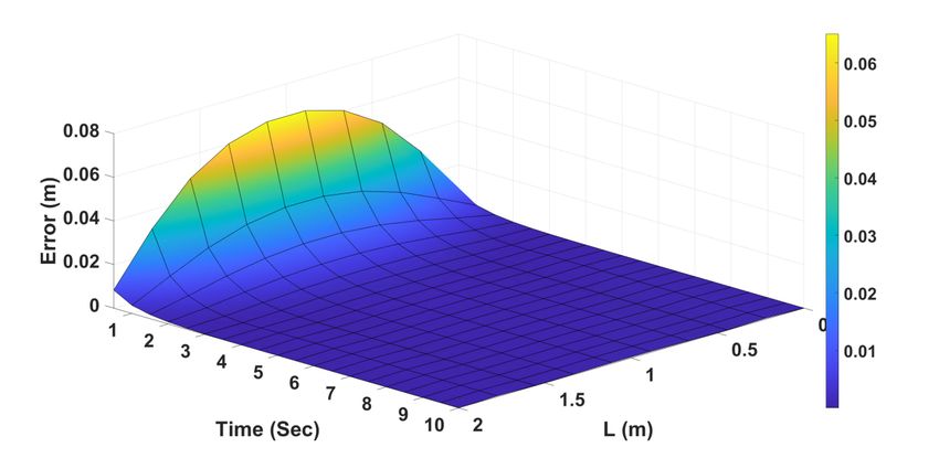
[8]. In the actions of a Hamiltonian system, the sym-          Also, u equals L at the opposite endpoint, provided
plectic integrator does not generate a secular trunca-         that L is the length of the DLO. This can be written
tion error. The number of force function evaluations           mathematically as:
of the fourth-order symplectic integrator is smaller                                           nu
than the ones of the Runge-Kutta integrator of the
                                                                                               X
                                                                                   q(u) =            bi (u)qi ,           (1)
same order. The energy conservation and the long-                                              i=1
time stability for the symplectic scheme are investi-
gated and verified in [2], [13], [11], and [9]. There          where q(u) = (x(u), y(u), z(u), θ(u)) = (r(u), θ(u)) is
are many merits for symplectic integrator which are            the fourth-dimensional configuration functional space
discussed and outlined in deeper detail in [3], [4], and       of the DLO. It includes the three linear coordinates
[27]. For these advantages, the use of the symplectic          x, y, z of the DLO position at point u, and the DLO’s
integrator is investigated in this paper for DLO sim-          axial twisting θ. Also, bi (u) is the ith spline poly-
ulation instead of the conventional integrators. To            nomial basis employed to describe the shape of the
this end, a comparison between the results obtained            DLO. Moreover, qi are properly chosen coefficients,
from this symplectic integrator and other types of             typically called control points, used to correctly inter-
integrators will be executed.                                  polate the shape of the DLO through the bi (u) basis
   The main objective of this paper is to compare the          functions. nu is the number of control points.
properties and results obtained by the symplectic in-             For a variety of reasons, this DLO mathematical
tegrator with the ones obtained with other numerical           model is highly successful. Firstly, the spatial deriva-
methods. This activity is justified by the fact that,          tives calculation is straightforward, i.e.
at the best of our knowledge, no data are available                                            nu
                                                                                                      (j)
                                                                                               X
in literature about the performances of numerical in-                            q (j) (u) =         bi (u)qi ,           (2)
tegration algorithms for DLOs. For the DLO mod-                                                i=1
eling, multivariate dynamic splines are used in this
paper. A comparison between the symplectic, Runge-             where q (j) is the j th derivative of q. In fact, it can be
Kutta, and Zhai methods is performed in two cases.             defined by the same coefficients and easy-to-compute
In the first case, the effect of gravitational and in-         derivatives of bi (u). Second, the spline basis propri-
ternal forces only are considered, while in the second         eties guarantee that the DLO model curvature, which
case the application of an external force in addition          represents the DLO’s physical behavior [1], is mini-
to the previously mentioned forces is considered.              mized. Third, this model enables the representation
   The remainder of this article is arranged as follows.       of a generalized nonlinear function with smoothness
Sec. 2 outlines the key features of the mathematical           characteristics as a linear combination of the non-
model of the DLO. The conversion from Lagrangian               linear function basis bi (u), which relies on the free
into Hamiltonian and the symplectic integrator are             variable u only, by the linear coefficients qi .
discussed in Sec 3. Moreover, Sec. 4 introduces the               Referring to the system’s Lagrange equations, the
preliminary simulation results and comparisons. Fi-            DLO’s dynamic model can be expressed as a function
nally, conclusions and future work are draft out in            of the control points qi as:
Sec. 5.
                                                                  d ∂K

                                                                                       ∂U
                                                                              = Fi −       ,        i = 1, 2, . . . , nu , (3)
                                                                  dt ∂ q̇i             ∂qi
2    Dynamic Model of the DLO                            where K is the total kinetic energy, Fi is the external
                                                         force that is applied to the ith control point, and U
A third-order spline basis can effectively represent the is the total potential energy acting on the DLO. This
shape of the DLO. It is a function of a free coordinate potential energy is generated due to the influence of
u. This coordinate u represents the position on the gravity, stretching, torsion, and bending effects on
DLO which is equal to zero at the first endpoint. the DLO.

                                                           3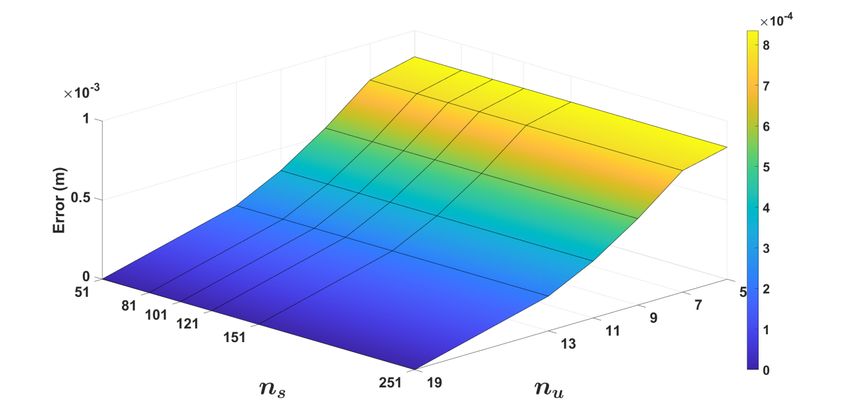
2.1 Kinetic Energy of the DLO where r and θ are the strain’s linear and the tor-
sional component, respectively. The strain energy
Owing to the translational motion of the control can therefore be written as:
points and the rotational motion of the cross sec-
tions, the total kinetic energy is generated. In order
to express this total kinetic energy, a function of the 1 L 1 L T
Z Z
T
U = ( − 0 ) H ( − 0 ) ds = He ds,
control points qi can be used as : 2 0 2 0 e
(7)
µ 0 0 0 where
1 L dq T dq
Z
E 0 0
0 µ 0 0
K= J ds, J = , 2
D π 2
2 0 dt dt 0 0 µ 0 H= 0 GD 8 0
0 0 0 I 4 ED 2
0 0 16
(4)
where J is the DLO’s generalized density matrix, ds 0 is the DLO’s plastic strain, which enables to con-
is the displacement element and can be computed sider the plasticity of the material. e is called the
0
from ds = kr (u)k du, µ denotes the linear density, residual strain that equals − 0 . Also, H is the ele-
and I denotes the polar moment of inertia. ment stiffness matrix, D is the cross-section diameter
According to the procedure explained in [28], we of the DLO. Moreover, E and G denote the Young’s
can drive: modulus and the shear modulus of the DLO’s mate-
X nu rial, respectively.
d ∂K
= Mij q̈j . (5) It is possible to write the right-side term of Eq. (3)
dt ∂ q̇i j=1 as:
Then, by expanding this definition to the overall
1 L ∂Te He
Z Z L T
system, the total inertial forces of the DLO can be ∂U ∂
Pi = − =− ds = − He ds,
written as M q̈, in which M denotes the inertia ma- ∂qi 2 0 ∂qi 0 ∂qi
trix of the DLO and q̈ is a vector that represents the (8)
control point accelerations. where Pi represents the elastic forces because of the
DLO deflection.
2.2 Potential Energy of the DLO
2.3 Dynamic Model of the DLO
The total potential energy U is made up of the grav-
To write the overall dynamic model of the DLO, the
itational effect and the strain energy of the DLO due
Eqs. (3), (5), and (8) are extended to the whole con-
to stretching, torsion and bending. Although the de-
trol points
rived energy of gravity is quite simple, the concept of
strain energy plays a crucial role in the modeling of
DLO. By introducing the strain vector = [s , t , b ] M q̈ = F + P (9)
that includes s to represent the stretching term, t where F refers to the vector that contains all exter-
to denotes the torsional term, and b to denotes the nal forces, including gravity, while P represents the
bending term such that: vector that contains all elastic forces.
At every simulation step, the system can be solved
by utilizing a simple LU decomposition. Moreover,
kCk
s = 1 − kr0 k , t = θ0 − γ, b = 3,
at each time step, the accelerations are integrated to
kr0 k get the control points velocities and positions. Sev-
(6)
0 00 C T r000 eral integration methods can be used, but some prob-
C =r ×r , γ= , lems may arise, including numerical instability, large
kCk2
4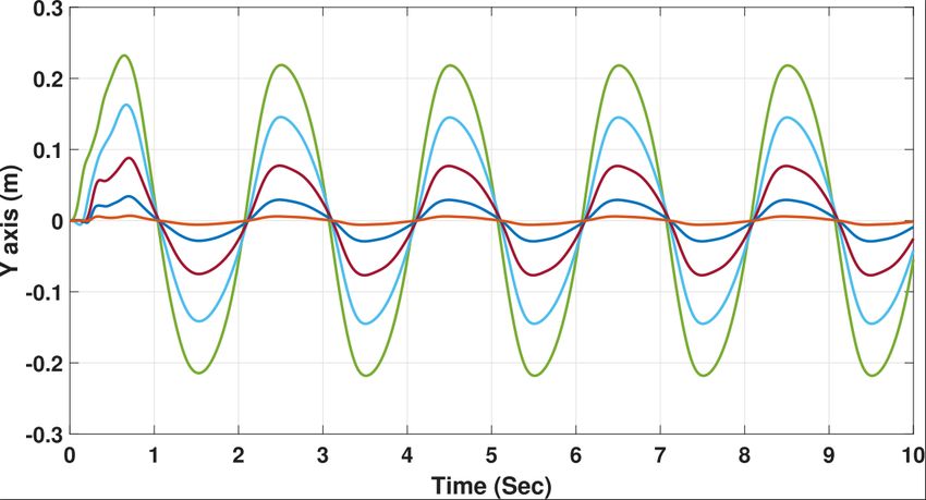
time required for the integration process and the un-
suitability for long-time predictions. These problems ∂Lg ∂K
pi (qi , q̇i ) = = . (12)
can be mitigated by using the symplectic integrator, ∂ q̇i ∂ q̇i
as will be shown in the following. The next section
will discuss this symplectic integrator and its require- 2. By inverting the expressions in the former step,
ments in more details. the velocities q̇i are formulated in terms of the
momenta pi .
3 Symplectic Integrator
pi = Jqi· so, q˙i = J −1 pi , (13)
To solve numerically the differential equations, we de-
1/µ 0 0 0
cided to use the symplectic integrator because of its 0 1/µ 0 0
advantages with respect to other methods as will be where J −1 = 0
.
0 1/µ 0
shown in the following. These subsections will dis-
0 0 0 1/I
cuss in detail calculating the Hamiltonian from La-
grangian and the construction of the symplectic inte- 3. Using the Lagrangian relation ( Lg = K − U ),
grator. we can conclude that:
1 L T
Z
3.1 Conversion from a Lagrangian to Lg = q̇ J q̇ ds − U. (14)
a Hamiltonian 2 0
Symplectic integrator is widely used in nonlinear dy-
The velocities q̇i are then substituted from Equ.
namics. It is designed as the numerical solution for
(13),
Hamilton’s equations, which provided as:
∂Hm ∂Hm 1
Z L
ṗ = − and q̇ = , (10) Lg = pT J −1 p ds − U. (15)
∂q ∂p 2 0
where p denotes the momentum coordinates, q refers
to the position coordinates, and Hm is the Hamilto- 4. The Hamiltonian is determined by employing the
nian which can be found from: typical definition of Hm as the Legendre trans-
formation of Lg :
Hm (p, q) = K(p) + U (q), (11)
where K and U denote the kinetic and potential en-
ergy, respectively. The set of position and momentum X ∂Lg X
Hm = q̇i − Lg = q̇i pi − Lg . (16)
coordinates (q, p) are named canonical coordinates. ∂ q̇i
In our case, the first step to use the symplectic inte-
grator is to make a conversion from Lagrangian into Substitution for q̇i from Equ. (13) and the La-
Hamiltonian [6]. This conversion is achieved accord- grangian Lg from Equ. (15) into Equ. (16), will
ing to the following procedure. lead to:
Provided a Lagrangian Lg as a function of the gen-
1 L T −1
Z
eralized coordinates qi and generalized velocities q̇i ,
Hm = p J p ds + U. (17)
where Lg (qi , q̇i ) = K (q̇i ) − U (qi ), the Hamiltonian 2 0
can be calculated according to the following steps:
1. By differentiating the Lagrangian Lg with re- The last equation is the require one as it is equiv-
spect to the generalized velocities q̇i , the mo- alent to the Hamiltonian equation that stated in
menta pi are determined: Equ. (11).
5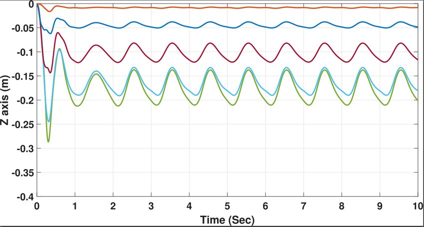
3.2     Symplectic Integrator                         of   the square of time. The symplectic integrator is thus well
        fourth-order                                suited to the long-time study of a dynamic system.
                                                    Generally, in the actions of a Hamiltonian system,
Forest [3] and Neri [27] introduced the generalized the symplectic integrator does not generate a secular
form of the fourth-order symplectic integrator as:  truncation error [20].

  q1 = q0 + c1 τ ∂K
                 ∂p (p0 ) ,          p1 = p0 − d1 τ ∂U
                                                    ∂q (q1 ) ,
                                                                      4    Simulation Results
  q2 = q1 + c2 τ ∂K
                 ∂p (p1 ) ,          p2 = p1 − d2 τ ∂U
                                                    ∂q (q2 ) ,        Numerical simulations have been carried out in MAT-
                                                                      LAB for the assessment of the mathematical frame-
  q3 = q2 + c3 τ ∂K
                 ∂p (p2 ) ,          p3 = p2 − d3 τ ∂U
                                                    ∂q (q3 ) ,        work discussed in the preceding sections. The issue
                                                                      that is aimed in this section is determining the DLO
  q4 = q3 + c4 τ ∂K
                 ∂p (p3 ) ,   p4 = p3 − d4 τ ∂U
                                             ∂q (q4 ) ,               state evolution, i.e. the control points evolution over
                                                   (18)               time, while influenced by a internal elastic and in-
where τ is the time step-size, q0 and p0 are the initial              ertial forces as well as external forces like gravita-
values, and q4 and p4 are the numerical solution af-                  tional force or contacts forces generated by obsta-
ter τ . Moreover, ci and di are numerical coefficients                cles. In the case of contacts, we can reshape the sys-
which can be determined uniquely from:                                tem as a constrained dynamic system in which the
                                                                      Lagrange approach for constraints is adopted. Just
                                                (1−β)
                                                                      add some constraints to the solution of the dynamic
                      1
       c1 = c4 =   2(2−β) ,    c2 = c3 =       2(2−β) ,               system. This will not change the problem, but just
                                                                      increase the number of dynamic equations that ex-
                    1                 −β                   (19)
      d1 = d3 =   (2−β) ,     d2 =   (2−β) ,    d4 = 0,               isted in the model. In [36], the solution of dynamic
                                                                      equations representing the DLO dynamics including
                    where β = 21/3 .                                  contacts is reported. The same approach can be ap-
                                                                      plied also to the symplectic integrator by changing
The reader can refer to the reference [4] for the deriva-             the dynamic equations accordingly. The simulations
tion and the values of the numerical coefficients.                    have been performed using the dynamic model in
   The number of force function evaluations ∂U   ∂q , that
                                                                      Eq. (9). It is worth mentioning that all simulations
is the most time-expensive operation in the integra-                  of this work have been performed on Ubuntu 18.04.5
tion process, is three rather than four since d4 = 0.                 LTS operating system, processor intel core i5-3210M
On the other hand, four force function evaluations                    CPU@2.50GHz x 4, RAM 8GiB.
are required in the conventional fourth-order Runge-                     In our simulations, DLO’s material is assumed to
Kutta integrator. Thus, the CPU time can be de-                       be aluminum, and its length L is 2 meters. The DLO
creased by approximately 25 percent with the sym-                     has a circular cross-section with a diameter D that
plectic integrator with respect to the fourth-order                   equals 2 millimeters. The number of control points
Runge-Kutta method.                                                   is selected as nu = 9. Also, the number of sam-
   Other than the energy-preserving property, a re-                   ple points along the DLO is chosen to be ns =101.
markable characteristic of the symplectic integrator                  These values are chosen to be sufficiently low but pro-
is that the aggregation of the truncation error in the                vide a good interpolation capability. During these
total energy has not a secular component and the po-                  simulations, the DLO is supposed to be placed ini-
sitional errors rise in proportional to the first order of            tially on a straight position along the x-axis, and
time [20]. On the other hand, conventional integra-                   the two extreme endpoints are constrained to move
tors generate a secular energy error. Moreover, the                   along the x-axis and attached by springs with stiff-
error due to position discretization increase with the                ness (Kx = 10 kN/m) to their initial position. In

                                                                  6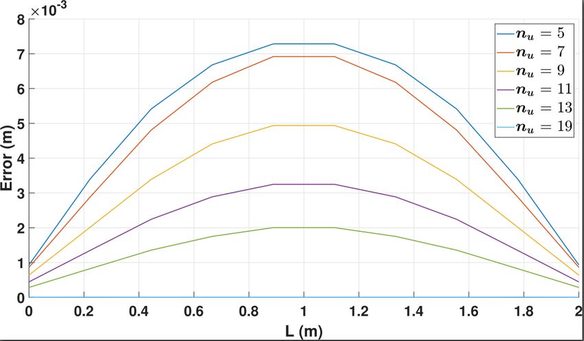
other words, one endpoint of the DLO is located at video that illustrates this numerical simulation, in
(0, 0, 0), while the opposite endpoint is located at case of applying an external force, is found in the
(L, 0, 0). Two simulation scenarios will be used in this link 2 . These results prove the ability of the spline-
section. In the first scenario, the DLO is affected by based dynamic model and the symplectic integrator
the internal forces and the gravitational force only as to represent the state evolution of the DLO accu-
shown in Fig. 1a. While in the second scenario, the rately. Fig. 8 shows the sequence of trajectories that
DLO is affected by the previously mentioned forces illustrate the DLO motion starting from the initial
in addition to an external sinusoidal force which is position according to the second scenario, i.e. the
applied to the DLO center in the Y-direction as illus- DLO is affected by the internal forces, the gravita-
trated in Fig. 1b. tional force, and an external sinusoidal force applied
Fig. 2, and 3 illustrate the computed solutions to the DLO center in the Y-direction.
accomplished utilizing the spline-based model us- The DLO model simulation time of the symplec-
ing symplectic integrator where the DLO is affected tic integrator is compared with the ones of both the
by the gravity and the internal forces only without classical Runge-Kutta integrator and Zhai integrator.
any other external forces. Fig. 2 presents the x- Zhai integrator is a new simple fast explicit time in-
component of each control point, while Fig. 3 shows tegration method, the reader can refer to [40] for the
the z-component of each control point. This sim- related details and advantages of Zhai integrator. In
ulation is achieved for 10 seconds using 2 millisec- MATLAB/Simulink, the three integrators are imple-
onds as a time step-size τ . This time step-size is the mented by using the same spline-based model defined
largest value that preserves the stability of the inte- in Sec. 2. In the case the DLO is affected by internal
gration method. It is worth mentioning that, during forces and gravity only, Table 1 reports the compari-
the whole period, the y component for each control son between the three integrators’ simulation time in
point is equal to zero as the DLO is positioned along seconds for a certain period (10 sec) with 2 millisec-
the x-axis and the external force is not applied yet. onds as a time step-size τ . The results show that the
In Fig. 3, due to the symmetry of the DLO, each symplectic integrator is faster than both the Runge-
two control points’ trajectories are located above each Kutta and Zhai integration methods. It is worth
other in one curve except the middle point. A video mentioning that the Zhai method needs optimization
that shows this numerical simulation exists in the link for two parameters [40] . However, we made a man-
1 ual tunning to these parameters. This may be the
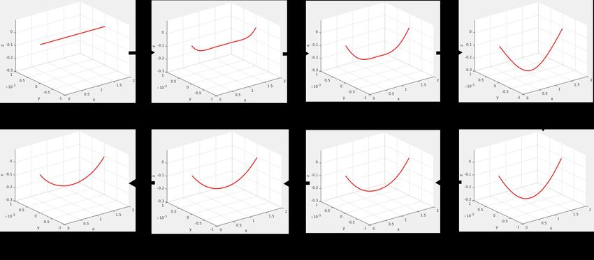
. Fig. 4 shows the sequence of trajectories that il-
lustrate the DLO motion starting from the initial po- reason for the notable slowness of Zhai compared to
sition according to the first scenario, i.e. the DLO is the Runge-Kutta method.
affected by the internal forces and the gravitational Table 2 presents the comparison between the three
force only without any other external forces. integrators’ computation time in seconds for a sim-
The simulation is performed again in the case of ap- ulation of 10 seconds in the case where the DLO
plying an external force on a DLO point. We assumed is affected by the external force in addition to the
that the external force takes the shape of a sinusoidal previously mentioned forces. The results show that
trajectory. This external force is applied to the cen- the symplectic integrator is able to solve the problem
ter of the DLO in the Y-axis direction. Fig. 5, 6, and while, on the other hand, the Runge-Kutta and Zhai
7 show the x, y, and z components, respectively. The integrators have been stuck and could not compute
solution discussed here assumes the knowledge of the any solution. It is worth mentioning that, in this
external forces F (the input). The computation will work, we did not investigate the reason why other
give the control points q (the output) that describe methods are unstable.
the DLO motion during the simulation interval. A The simulation implemented in MATLAB, using
1 https://www.dropbox.com/s/4tb3ohyod5v71yj/ 2 https://www.dropbox.com/s/b1tc8v1k627o33r/
videoforspline.avi?dl=0 videoforspline.avi?dl=0
7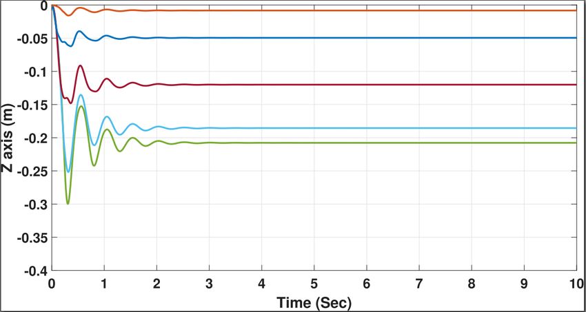
Figure 1: Schematic diagram of the DLO in which it is affected by: a) gravitational force, and b) gravitational
force and the DLO’s center is affected by an external force in the Y direction.

Figure 2: X component of each control point of the        Figure 3: Z component of each control point of the
DLO.                                                      DLO.

                                                      8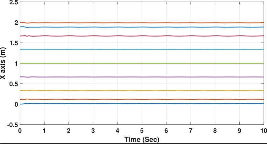
Figure 4: Sequence of trajectories to show the DLO motion starting from the initial position according to
the first scenario.

Figure 5: X component of each control point of the Figure 6: Y component of each control point of the
DLO in which its center is affected by external sinu- DLO in which its center is affected by external sinu-
soidal force.                                         soidal force.

                                                    9
internal forces only and sinusoidal external force, re-
spectively. Each cell in the two tables introduces the
execution time in seconds for a simulation period of
10 seconds. Likewise, Table 7, and 8 illustrate C++
results of execution time with changing nu and ns .
From these tables, we conclude that C++ is faster
about three times more than MATLAB implemen-
tations. So, C++ implementation with symplectic
integrator will be better for the practical implemen-
tation of the simulation system. Moreover, reducing
nu and/or ns will require less execution time, but it
will reduce interpolation precision in representing the
DLO. It is worth mentioning that the time step size is
chosen to be unique and equal to 0.8 milliseconds for
all of these comparisons. As nu and ns are increased,
Figure 7: Z component of each control point of the more calculations are required and hence the integra-
DLO in which its center is affected by external sinu- tion time increases. The same step size is selected for
soidal force. all comparisons for fairness.
The model with the highest resolution (ns = 256
and nu = 19) is considered as the reference model.
the fastest integrator, takes an average time of 470 Each model resolution considered in this work is com-
seconds for the simulation of 10 seconds like the one pared to the reference model and the error is com-
reported in Fig. 2 and 3. This long execution time puted. For each resolution, the DLO position is mea-
occurs due to two reasons. The first reason is the sured at 10 fixed points along the DLO. Moreover,
specifications of the processing unit or the PC. The the error over time is computed by considering 20
second reason is the implementation on MATLAB equidistant time intervals. Fig. 9 shows the evolu-
which is not really efficient. To avoid this reason, an- tion of this error over the time and the DLO length.
other simulation is repeated using C++ language. In It is noticed that the maximum error occurred at the
these simulations and in the related comparisons, the center of the DLO and the error decreases over time.
Zhai integrator is excluded as it is the slowest and it The evolution of the error with different values for
looks not really efficient in solving the DLO dynam- ns and nu is presented in Fig. 10. As nu increases,
ics. Hence, the current comparison will be focused the error decreases and vice versa, while ns has no
on the symplectic and the Runge-Kutta integration noticeable effect on the error. Moreover, as the num-
methods and their implementation in C++. Tables 3 ber of control points nu increases, the error decreases
and 4 introduce the comparison between the two in- over time and with respect to the position along the
tegrators’ execution time in the case of internal forces DLO as indicated in Fig. 11 and 12, respectively.
only and sinusoidal external force, respectively. From
Tables 3 and 4, it can be concluded that the symplec-
tic integrator gives the fastest execution time. Also, 5 Conclusions
the C++ execution time is reduced to be one-third
of the execution time of MATLAB results. This paper reports a comparison among integration
To check the effect of changes in the DLO model methods to solve the dynamic model of Deformable
granularity, nu and ns on the execution time, simu- Linear Objects. The adopted DLO model is based
lations on both MATLAB and C++ are performed. on the multivariate dynamic spline and employs the
Tables 5 and 6 present MATLAB results of the exe- symplectic integrator. This symplectic integrator re-
cution time by changing nu and ns for both cases of ceived particular attention due to its advantages over
10Figure 8: Sequence of trajectories to show the DLO motion starting from the initial position according to
the second scenario.
Figure 9: Evolution of the error over time and DLO Figure 10: Evolution of the error over ns and nu
length. points.
11Table 1: MATLAB execution time for solving the
DLO model employing different integrators without
applying an external force.
Simulation time Symplectic Runge-Kutta Zhai
0.1 6.66 9.43 34.85
0.2 11.39 16.42 67.57
0.3 16.14 22.43 96.69
0.4 20.86 28.41 120.45
0.5 25.60 34.62 145.42
0.6 30.42 41.29 166.22
0.7 35.17 48.62 186.46
0.8 39.92 56.07 206.70
0.9 44.61 62.59 226.81
1 49.30 68.89 247.39
2 97.18 140.00 478.94
3 144.21 210.41 685.46
4 191.20 278.22 904.89
5 238.24 347.53 1127.37
6 285.31 418.16 1348.17
7 332.29 487.72 1542.90
8 379.23 555.20 1733.71
9 426.17 624.36 1970.40
Figure 11: Evolution of the error over time at differ- 10 473.18 697.04 2204.93
ent nu points.
alternative methods in solving the dynamic equations
of Hamiltonian systems. Simulations on MATLAB
and using C++ code are performed to compare the
performance of the symplectic integrator against the
Runge-Kutta and Zhai integrators. The results prove
that the symplectic integrator is the fastest and the
most stable integrator among the considered ones.
Moreover, the proposed comparison shows that C++
is about three times faster than the corresponding
MATLAB implementation. Hence, a spline-based
model with a symplectic integrator looks to be the
best choice for practical implementation. Finally,
comparisons are performed to check the effects of
changing the model granularity. These results show
that reducing the control points and sample points
will reduce the execution time, but it will reduce the
interpolation precision in representing the DLO be-
havior.
In future work, practical experiments will be used
Figure 12: Evolution of the error over DLO length at to validate the spline-based model and the results ob-
different nu points. tained with the symplectic integrator. Moreover, this
model will be exploited to optimize the DLO manip-
ulation process. Also, an extension to the method
will be applied to multi-branch DLOs, like the pre-
12Table 4: C++ execution time for solving the DLO
Table 2: MATLAB execution time for solving the model employing different integrators in case of ap-
DLO model employing different integrators in case of plying an external force.
applying an external force. Simulation time Symplectic Runge-Kutta
Simulation time Symplectic Runge-Kutta Zhai 0.1 1.98 5.45
0.1 6.83
0.2 3.98 9.85
0.2 11.75
0.3 16.70 0.3 5.92 13.63
0.4 21.64 0.4 7.93 16.88
0.5 26.60 0.5 9.99 20.12
0.6 31.56 0.6 11.91 23.42
0.7 36.55
0.7 13.97 26.81
0.8 41.48
0.9 46.44 0.8 15.99 30.52
1 51.40 Unstable Unstable 0.9 17.90 34.53
2 101.14 1 19.90 38.17
3 150.73 2 40.10 76.95
4 200.30
3 60.16 115.53
5 249.89
6 298.60 4 80.41 154.16
7 346.63 5 101.47 193.16
8 394.63 6 123.51 231.97
9 442.50 7 146.46 270.46
10 490.59 8 167.34 309.58
9 189.53 349.07
10 210.46 388.04
Table 3: C++ execution time for solving the DLO
Table 5: Effects of changing the model parameters
model employing different integrators without apply-
(nu &ns ) on MATLAB execution time for solving
ing an external force.
the DLO model employing the symplectic integrator
Simulation time Symplectic Runge-Kutta
without applying an external force.
0.1 2.04 5.88
ns
0.2 3.85 10.44 nu 51 81 101 121 151 251
0.3 5.65 13.90 5 488.28 688.22 825.99 960.52 1288.93 2094.12
0.4 7.55 16.75 7 588.53 811.56 998.6 1201.32 1419.81 2357.17
0.5 9.38 19.93 9 713.17 967.77 1299.68 1421.18 1634.21 2787.05
11 770.00 1129.01 1344.34 1691.19 2033.16 3171.8
0.6 11.17 23.09 13 908.49 1332.11 1566.67 1893.44 2304.9 3909.13
0.7 12.95 26.43 19 1331.77 1714.65 2348.26 2479.57 3104.75 5090.28
0.8 14.73 29.82
0.9 16.56 33.00
1 18.35 36.39 Table 6: Effects of changing the model parameters
2 36.57 69.57 (nu &ns ) on MATLAB execution time for solving the
3 54.67 102.85 DLO model employing the symplectic integrator in
4 72.88 136.00 case of applying an external force.
5 90.99 169.06
ns
6 109.11 201.95 nu
51 81 101 121 151 251
7 127.30 235.07 5 489.98 677.93 888.11 1004.88 1254.07 2015.19
8 145.86 268.21 7 538.59 881.56 1007.06 1214.88 1554.83 2379.88
9 643.93 970.64 1124.15 1405.01 1675.14 2970.31
9 164.16 301.24 11 717.9 1101.62 1385.67 1692.81 2006.02 3140.75
10 182.46 334.40 13 874.72 1291.78 1568.77 1886.01 2313.28 3903.67
19 1386.62 1826.59 2102.17 2667.17 2990.85 5035.5
13assembled wiring harness utilized in the aerospace
and automotive industries.
acknowledgment
Table 7: Effects of changing the model parameters This work was supported by the European Commis-
(nu &ns ) on C++ execution time for solving the DLO sions Horizon 2020 Framework Programme with the
model employing the symplectic integrator without project REMODEL - Robotic technologies for the
applying an external force. manipulation of complex deformable linear objects -
ns under grant agreement No 870133.
nu 51 81 101 121 151 251
5 155.28 232.5 284.52 339.25 416.16 673.25
7 197.56 295.17 363.86 435.05 529.7 861.73
9 245.61 369.37 455.4 523.42 652.07 1065.55
11 286.957 436.69 534.16 623.1 765.75 1271.19 References
13 319.786 489.52 601.8 713.24 887.17 1437.82
19 450.95 690.64 840.81 990.89 1236.14 2021.42 [1] Carl De Boor. A practical guide to splines; rev.
ed., ser. applied mathematical sciences. 2001.
[2] Kang Feng. On difference schemes and symplec-
tic geometry. In Proceedings of the 5th interna-
tional symposium on differential geometry and
differential equations, 1984.
[3] Etienne Forest. Canonical integrators as track-
ing codes (or how to integrate perturbation the-
ory with tracking). Technical report, Lawrence
Berkeley Lab., 1987.
[4] Etienne Forest and Ronald D Ruth. Fourth-
Table 8: Effects of changing the model parameters order symplectic integration. Physica D: Non-
(nu &ns ) on C++ execution time for solving the DLO linear Phenomena, 43(1):105–117, 1990.
model employing the symplectic integrator in case of
applying an external force. [5] Leopoldo Greco and Massimo Cuomo. B-spline
ns interpolation of kirchhoff-love space rods. Com-
nu
51 81 101 121 151 251 puter Methods in Applied Mechanics and Engi-
5 154.18 231.83 283.43 335.97 414.29 680.41 neering, 256:251–269, 2013.
7 195.2 295.25 361.43 427.65 530.54 863.73
9 238.25 358.64 442.07 521.7 645.43 1060.26
11 278.72 426.39 523.94 617.38 764.78 1253.72 [6] Patrick Hamill. A student’s guide to Lagrangians
13 319.12 488.51 600.33 709.03 889.24 1436.29 and Hamiltonians. Cambridge University Press,
19 442.82 677.01 835.82 988.3 1228.88 2023.9 2014.
[7] Tomas Hermansson, Robert Bohlin, Johan S
Carlson, and Rikard Söderberg. Automatic as-
sembly path planning for wiring harness in-
stallations. Journal of manufacturing systems,
32(3):417–422, 2013.
14[8] Jialin Hong, Chuying Huang, and Xu Wang. manipulation of deformable objects. In 2015
Symplectic runge–kutta methods for hamilto- IEEE/RSJ International Conference on Intelli-
nian systems driven by gaussian rough paths. gent Robots and Systems (IROS), pages 878–885.
Applied Numerical Mathematics, 129:120–136, IEEE, 2015.
2018.
[17] Jagadeesan Jayender, Rajnikant V Patel, and
[9] Weipeng Hu, Zichen Deng, Songmei Han, and Suwas Nikumb. Robot-assisted active catheter
Wenrong Zhang. Generalized multi-symplectic insertion: Algorithms and experiments. The
integrators for a class of hamiltonian nonlinear International Journal of Robotics Research,
wave pdes. Journal of Computational Physics, 28(9):1101–1117, 2009.
235:394–406, 2013.
[18] Xin Jiang, Kyong-mo Koo, Kohei Kikuchi, At-
[10] Weipeng Hu, Zhen Wang, Yunping Zhao, and sushi Konno, and Masaru Uchiyama. Robotized
Zichen Deng. Symmetry breaking of infinite- assembly of a wire harness in a car production
dimensional dynamic system. Applied Mathe- line. Advanced Robotics, 25(3-4):473–489, 2011.
matics Letters, 103:106207, 2020.
[19] P Jiménez. Survey on model-based manipulation
[11] Weipeng Hu, Mengbo Xu, Jiangrui Song, Qiang planning of deformable objects. Robotics and
Gao, and Zichen Deng. Coupling dynamic computer-integrated manufacturing, 28(2):154–
behaviors of flexible stretching hub-beam sys- 163, 2012.
tem. Mechanical Systems and Signal Processing,
151:107389, 2021. [20] Hiroshi Kinoshita, Haruo Yoshida, and Hiroshi
Nakai. Symplectic integrators and their applica-
[12] Weipeng Hu, Juan Ye, and Zichen Deng. In-
tion to dynamical astronomy. Celestial Mechan-
ternal resonance of a flexible beam in a spatial
ics and Dynamical Astronomy, 50:59–71, 1991.
tethered system. Journal of Sound and Vibra-
tion, 475:115286, 2020. [21] Joachim Linn and Klaus Dreßler. Discrete
[13] Weipeng Hu, Tingting Yin, Wei Zheng, and cosserat rod models based on the difference ge-
Zichen Deng. Symplectic analysis on orbit- ometry of framed curves for interactive simula-
attitude coupling dynamic problem of spatial tion of flexible cables. In Math for the Digital
rigid rod. Journal of Vibration and Control, Factory, pages 289–319. Springer, 2017.
26(17-18):1614–1624, 2020. [22] Wen Hao Lui and Ashutosh Saxena. Tangled:
[14] Weipeng Hu, Lingjun Yu, and Zichen Deng. Learning to untangle ropes with rgb-d percep-
Minimum control energy of spatial beam with tion. In 2013 IEEE/RSJ International Confer-
assumed attitude adjustment target. Acta Me- ence on Intelligent Robots and Systems, pages
chanica Solida Sinica, 33(1):51–60, 2020. 837–844. IEEE, 2013.
[15] Weipeng Hu, Chuanzeng Zhang, and Zichen [23] Naijing Lv, Jianhua Liu, Xiaoyu Ding, Jiashun
Deng. Vibration and elastic wave propagation in Liu, Haili Lin, and Jiangtao Ma. Physically
spatial flexible damping panel attached to four based real-time interactive assembly simulation
special springs. Communications in Nonlinear of cable harness. Journal of Manufacturing Sys-
Science and Numerical Simulation, 84:105199, tems, 43:385–399, 2017.
2020.
[24] Naijing Lv, Jianhua Liu, Huanxiong Xia, Jiang-
[16] Sandy H Huang, Jia Pan, George Mulcaire, tao Ma, and Xiaodong Yang. A review of tech-
and Pieter Abbeel. Leveraging appearance pri- niques for modeling flexible cables. Computer-
ors in non-rigid registration, with application to Aided Design, 122:102826, 2020.
15[25] Rene J Moreno Masey, John O Gray, Tony J [33] JM9728120655 Sanz-Serna. Runge-kutta
Dodd, and Darwin G Caldwell. Guidelines for schemes for hamiltonian systems. BIT Numeri-
the design of low-cost robots for the food indus- cal Mathematics, 28(4):877–883, 1988.
try. Industrial Robot: An International Journal,
2010. [34] Martin Servin and Claude Lacoursiere. Rigid
body cable for virtual environments. IEEE
[26] Mark Moll and Lydia E Kavraki. Path planning Transactions on Visualization and Computer
for deformable linear objects. IEEE Transac- Graphics, 14(4):783–796, 2008.
tions on Robotics, 22(4):625–636, 2006.
[35] Ankit Shah, Lotta Blumberg, and Julie Shah.
[27] Filippo Neri. Lie algebras and canonical integra- Planning for manipulation of interlinked de-
tion. Dept. of Physics, University of Maryland, formable linear objects with applications to air-
1987. craft assembly. IEEE Transactions on Automa-
tion Science and Engineering, 15(4):1823–1838,
[28] Olivier Nocent and Yannick Remion. Contin- 2018.
uous deformation energy for dynamic material
[36] Adrien Theetten, Laurent Grisoni, Claude An-
splines subject to finite displacements. In Com-
driot, and Brian Barsky. Geometrically ex-
puter Animation and Simulation 2001, pages 87–
act dynamic splines. Computer-Aided Design,
97. Springer, 2001.
40(1):35–48, 2008.
[29] Gianluca Palli. Model-based manipulation of de- [37] Adrien Theetten, Laurent Grisoni, Christian
formable linear objects by multivariate dynamic Duriez, and Xavier Merlhiot. Quasi-dynamic
splines. In 2020 IEEE Conference on Industrial splines. In Proceedings of the 2007 ACM sympo-
Cyberphysical Systems (ICPS), volume 1, pages sium on Solid and physical modeling, pages 409–
520–525. IEEE, 2020. 414, 2007.
[30] Matthias Rambow, Thomas Schauß, Martin [38] Pier Paolo Valentini and Ettore Pennestrı̀. Mod-
Buss, and Sandra Hirche. Autonomous manip- eling elastic beams using dynamic splines. Multi-
ulation of deformable objects based on teleop- body system dynamics, 25(3):271–284, 2011.
erated demonstrations. In 2012 IEEE/RSJ In-
ternational Conference on Intelligent Robots and [39] Weifu Wang, Dmitry Berenson, and Devin Balk-
Systems, pages 2809–2814. IEEE, 2012. com. An online method for tight-tolerance in-
sertion tasks for string and rope. In 2015 IEEE
[31] Arnau Ramisa, Guillem Alenya, Francesc International Conference on Robotics and Au-
Moreno-Noguer, and Carme Torras. Using depth tomation (ICRA), pages 2488–2495. IEEE, 2015.
and appearance features for informed robot
[40] Wanming Zhai. Numerical method and com-
grasping of highly wrinkled clothes. In 2012
puter simulation for analysis of vehicle–track
IEEE International Conference on Robotics and
coupled dynamics. In Vehicle–track coupled dy-
Automation, pages 1703–1708. IEEE, 2012.
namics, pages 203–229. Springer, 2020.
[32] Jose Sanchez, Juan-Antonio Corrales,
Belhassen-Chedli Bouzgarrou, and Youcef
Mezouar. Robotic manipulation and sensing of
deformable objects in domestic and industrial
applications: a survey. The International
Journal of Robotics Research, 37(7):688–716,
2018.
16You can also read