HydroGFD3.0 (Hydrological Global Forcing Data): a 25 km global precipitation and temperature data set updated in near-real time - ESSD
←
→
Page content transcription
If your browser does not render page correctly, please read the page content below
Earth Syst. Sci. Data, 13, 1531–1545, 2021
https://doi.org/10.5194/essd-13-1531-2021
© Author(s) 2021. This work is distributed under
the Creative Commons Attribution 4.0 License.

       HydroGFD3.0 (Hydrological Global Forcing Data): a 25 km
            global precipitation and temperature data set
                      updated in near-real time
                                      Peter Berg, Fredrik Almén, and Denica Bozhinova
             Swedish Meteorological and Hydrological Institute, Folkborgsvägen 17, 60176 Norrköping, Sweden
                                       Correspondence: Peter Berg (peter.berg@smhi.se)

                                 Received: 13 August 2020 – Discussion started: 21 September 2020
                          Revised: 3 February 2021 – Accepted: 11 February 2021 – Published: 13 April 2021

       Abstract. HydroGFD3 (Hydrological Global Forcing Data) is a data set of bias-adjusted reanalysis data for
       daily precipitation and minimum, mean, and maximum temperature. It is mainly intended for large-scale hy-
       drological modelling but is also suitable for other impact modelling. The data set has an almost global land
       area coverage, excluding the Antarctic continent and small islands, at a horizontal resolution of 0.25◦ , i.e. about
       25 km. It is available for the complete ERA5 reanalysis time period, currently 1979 until 5 d ago. This period will
       be extended back to 1950 once the back catalogue of ERA5 is available. The historical period is adjusted using
       global gridded observational data sets, and to acquire real-time data, a collection of several reference data sets is
       used. Consistency in time is attempted by relying on a background climatology and only making use of anomalies
       from the different data sets. Precipitation is adjusted for mean bias as well as the number of wet days in a month.
       The latter is relying on a calibrated statistical method with input only of the monthly precipitation anomaly such
       that no additional input data about the number of wet days are necessary. The daily mean temperature is adjusted
       toward the monthly mean of the observations and applied to 1 h time steps of the ERA5 reanalysis. Daily mean,
       minimum, and maximum temperature are then calculated. The performance of the HydroGFD3 data set is on par
       with other similar products, although there are significant differences in different parts of the globe, especially
       where observations are uncertain. Further, HydroGFD3 tends to have higher precipitation extremes, partly due
       to its higher spatial resolution. In this paper, we present the methodology, evaluation results, and how to access
       the data set at https://doi.org/10.5281/zenodo.3871707 (Berg et al., 2020).

1   Introduction                                                       While most data sets now offer a rather long historical pe-
                                                                    riod, the real-time availability is a greater challenge. Merged
Precipitation (P ) and temperature (T ) are key driving param-      satellite and gauge data sets such as CHIRPS (Funk et al.,
eters for many impact models, and there are now many obser-         2015a), CMORPH (Joyce et al., 2004), and PERSIANN-
vational data sets available. They differ regarding the spatio-     CDR (Ashouri et al., 2015) offer both high-resolution and
temporal resolution, the historical coverage, and the data          near-real-time components but are limited to between the
sources included in the product. However, when it comes to          ±50◦ or ±60◦ latitude bands. Several data sets have made
continuously updated near-real-time data sets, there are very       use of reanalysis data as a basis, adjusted using various grid-
few available data sets. It is therefore challenging to find a      ded observational data sets (Weedon et al., 2011, 2014; Beck
product suitable for monitoring and initialization of forecasts     et al., 2017; Berg et al., 2018; Cucchi et al., 2020). The ad-
for an impact model, i.e. a product that fulfils both a long his-   vantage is that the reanalysis products are readily available
torical period for calibration and validation as well as real-      with a large range of variables and output frequencies. Still,
time updates.                                                       the downside with reanalysis products is that especially P is
                                                                    a model product and thereby suffers from model bias. Since

Published by Copernicus Publications.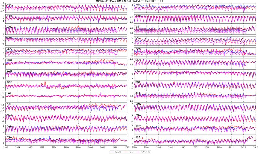
1532                                                                                                P. Berg et al.: HydroGFD3.0

the bias can be substantial, several methods have been devel-      (Hersbach et al., 2020) and forms the basis for HydroGFD3.
oped to adjust reanalysis using different methods and refer-       This reanalysis product is chosen because our operational
ence data sets.                                                    forecasts at the SMHI (Swedish Meteorological and Hydro-
   A hydrological-operational-monitoring or forecast prod-         logical Institute) are based on the medium-range forecasts of
uct has strong demands on availability and redundancy of           the ECMWF, with the same model as that used for ERA5
the data flows. The data set HydroGFD1 (Hydrological               and a similar bias, although there are differences in model
Global Forcing Data; Berg et al., 2018) was constructed            version. Other reanalysis products would be possible but are
and made operational for initializations of the hydrologi-         not explored here. ERA5 is updated with a 3-month lag, but
cal model HYPE (HYdrological Predictions for the Environ-          a new temporary product, ERA5T, is produced with a 5 d lag.
ment) (Lindström et al., 2010) for different set-ups across           As described in Sect. 3, HydroGFD3 is based on a combi-
the globe. It offered near-real-time updating of daily P and       nation of the ERA5 reanalysis with the different data sets as
daily T (mean, minimum, and maximum) until the end of              listed in the top section of Table 1. In the following analysis,
the last calendar month. The real-time components of Hy-           we compare the different data sets included in the process-
droGFD1 were based on ERA-Interim reanalysis, extended             ing and additionally make a state-of-the-art comparison to
by the ECMWF deterministic forecasts and adjusted us-              the data set WFDE5 (Cucchi et al., 2020), which is a new
ing monthly mean P from GPCC-Monitoring and GPCC-                  product using the WATCH forcing data methodology (Wee-
FirstGuess (Schneider et al., 2018b) products and monthly          don et al., 2011) with ERA5 reanalysis, listed in the bottom
mean T from GHCN–CAMS (the Global Historical Climate               section of Table 1.
Network combined with the Climate Anomaly Monitoring                  An issue with global-scale evaluations is that of indepen-
System) (Fan and Van den Dool, 2008). The follow-up data           dence between data sets, and most of the gauge-based data
set HydroGFD2 offered some updates to the methodology              sets listed in Table 1 make use of more or less the same
and shifted to using primarily the CPC-Unified (Chen et al.,       openly available observations, with regional differences. The
2008) and CPC-Temp (CPCtemp, 2017) products for P and              data sets have, however, been independently generated and
T adjustments, respectively. Both data sets employed a 0.5◦        use different statistical models for the gridding process. Our
resolution and have been operationally produced for a few          aim is to provide a comprehensive overview of HydroGFD3
years now, and we have identified some serious issues re-          in comparison to other data sets in order to present its quali-
garding the availability of required data sets for successful      ties and to point out potential issues. For each of the compar-
updates. The largest operational intermission occurred dur-        isons in Sect. 5, we chose data sets that are as independent as
ing the government lockdown in the US between 22 Decem-            possible given the limitations just discussed. Our experience
ber 2018 and 25 January 2019. Neither of the US data sets          from earlier studies is that in-depth evaluation can only be
included in the production were then available, which ham-         performed at the local scale (e.g. Fallah et al., 2020), and we
pered the production of the HydroGFD data sets and subse-          encourage users of the data set to pursue such evaluations.
quently deteriorated the quality of some operational HYPE
models. Both these HydroGFD versions have now become               3     Method
obsolete for real-time production due to the discontinuation
of the ERA-Interim production as of August 2019. Data sets         The main method that HydroGFD3 is building on consists of
using multiple input data sources are less sensitive to such       adding observational monthly anomalies to a background cli-
conditions, such as the MSWEP (Multi-Source Weighted-              matology, then adjusting the reanalysis data to that absolute
Ensemble Precipitation) data set (Beck et al., 2017).              monthly mean. Time steps shorter than the monthly mean are
   In this paper, the HydroGFD3.0 system is described, with        implicitly adjusted following the monthly scaling. A monthly
its range of produced data sets for the period 1979 to near        timescale is adopted due to the generally higher availability
real time at 0.25◦ resolution and global land coverage. We         of observational data sets at this resolution. Further steps as-
describe the methodology and the operational production as         sure consistency between different versions of the data set,
well as an evaluation of the climatological data set, with com-    e.g. regarding spatial coverage. The different steps in pro-
parison to other similar data sources.                             ducing the HydroGFD3 data sets are presented in detail in
                                                                   the following sections.

2   Data
                                                                   3.1    Climatology
Table 1 lists the data sources used in the production of the       The P background climatology is based on chpclim cli-
different tiers (i.e. production lines with different data sets;   matology of satellite, gauge, and physiographic indicators
see Methods section) of HydroGFD3. From now on, we use             (Funk et al., 2015b). We retain the same climatological pe-
the shortened internal abbreviations listed under “Name” in        riod (1980–2009) throughout the HydroGFD3 data set. The
Table 1 when we refer to the data of P or T from each source.      chpclim data set comes in two versions: one with full cov-
ERA5 is the latest global reanalysis product of the ECMWF          erage for the 50◦ S–50◦ N latitude band and one with global

Earth Syst. Sci. Data, 13, 1531–1545, 2021                                         https://doi.org/10.5194/essd-13-1531-2021
P. Berg et al.: HydroGFD3.0                                                                                                                   1533

Table 1. Table of model and data sources used in the production of HydroGFD3 as well as the WFDE5 data set used for comparison. Note
the lower-case abbreviations used in the main text and in figures, which follow the internal notation used in the data set production. Nwet is
a measure of the number of wet days in a month. The data set type is marked in parentheses in the leftmost column; r: model reanalysis; g:
gauge-based; s: satellite-based. Today’s date is marked by “t” in the “Period” column.

      Data set                  Name           Variables      Resolution              Period                       Data reference
      ERA5(r)                   e5             T, P           1 h; 0.33◦              1979–(t − 3 months)          C3S (2020b)
      ERA5T(r)                  e5t            T, P           1 h; 0.33◦              (t − 3 months) – (t − 5 d)   C3S (2020b)
      CRUts4.03(g)              cru            T , P , Nwet   1 month; 0.5◦           1901–(t − 2 months)          Harris and Jones (2019)
      GPCCv8(g)                 gpcch          P              1 month; 0.25◦          1891–2016                    Schneider et al. (2018a)
      GPCC-monitoringv6(g)      gpccm          P              1 month; 1.0◦           1982–(t − 3 months)          Schneider et al. (2018b)
      GPCC-First guess(g)       gpccf          P              1 month; 1.0◦           2004–(t − 1 month)           Schneider et al. (2018b)
      CPC-Unified(g)            cpcp           P              1 d; 0.5◦               1979–(t − 2 d)               CPC (2020)
      CPC-Temp(g)               cpct           Tmin , Tmax    1 d; 0.5◦               1979–(t − 2 d)               CPC (2017)
      CHPclimv1.0(g,s)          chpclim        P              climatological; 0.05◦   (1980–2009)                  Funk et al. (2015b)
      WFDE5-CRU(r,g)            wfde5-cru      T, P           1 h; 0.5◦               1979–2018                    C3S (2020a)
      WFDE5-GPCC(r,g)           wfde5-gpcc     P              1 h; 0.5◦               1979–2016                    C3S (2020a)

land coverage. We choose to make the global-coverage ver-                  between the data sets, sharp changes in the data are unavoid-
sion the main choice but add information from the tropical                 able when switching from one data set to another. The ho-
full-coverage version to increase coverage along coastlines                mogenization used here is performed by only making use of
and islands. The original 0.05◦ resolution is remapped to the              anomalies from the different data sets.
0.25◦ resolution of the HydroGFD3 data set, ensuring con-                     In the earlier version HydroGFD1 (Berg et al., 2018),
servation of precipitation totals. Some issues with the chp-               which is closely based on the WFD (WATCH Forcing Data)
clim data set were identified through visual inspection, with              method (Weedon et al., 2011), each month of the reanalysis
observational artefacts in mid-northern Siberia and underes-               data set is adjusted with the absolute monthly mean of the
timation in Scandinavia. Therefore, these two regions were                 observational data set. This main principle is retained; how-
replaced by gpcch climatological data for the 1980–2009 pe-                ever, in a new homogenization step we create new absolute
riod (see Supplement for details). To avoid introducing sharp              observations by first calculating the monthly anomaly com-
borders, a zone of five grid points was used around each                   pared to the 1980–2009 climatological period calculated for
area as a linear transition from one data set to another. Since            each data set, then adding this anomaly to the HydroGFD3
Greenland P is poorly mapped by both satellite and gauge                   climatology. Anomalies are additive for T ,
data, we have chosen to let its climatology be defined by e5
rather than any of the data sets.                                          Tanom (year, month) = T (year, month) − Tclim (month),              (1)
   For T , we use the cpct climatology (1980–2009) with only
                                                                           and multiplicative for P ,
a remapping to the 0.25◦ resolution and in-filling of miss-
ing data points using e5. The third climatology consists of                Panom (year, month) = P (year, month)/Pclim (month).                (2)
the wet-day frequency (1980–2009), which is taken from the
Nwet of the cru data set of gridded station observations of the               The reverse operation is applied after replacing the clima-
number of wet days in a month. Both T and P are remapped                   tology.
to the 0.25◦ resolution using a bilinear-interpolation method.
   In a final step, the three climatologies are harmonized by              3.3   Wet-day frequency
only retaining the grid points that are available consistently
in all data sets and all months. This leads also to the final land         A common issue with coarse-resolution models, such as e5,
mask of the HydroGFD3 data set, for which adjusted data are                is a tendency to produce excessive drizzle that reduces the
produced.                                                                  number of dry days in a month. To alleviate potential exces-
   The elevation is defined by the e5 surface geopotential di-             sive drizzle, the number of wet days is adjusted before cor-
vided by the gravity of Earth (9.80665 m/s2 ).                             recting the P amount. This is performed by first determining
                                                                           the target number of wet days in the month, then setting the
                                                                           days with weakest precipitation intensity to 0 until the target
3.2   Anomaly method                                                       is reached. No adjustments are made for too few wet days.
                                                                           The wet-day frequencies in a month are not well covered by
HydroGFD3 makes use of several different data sets, which                  observational monitoring records, and the uncertainties are
need to be stitched together in different configurations de-               large when available. We have chosen to estimate the num-
pending on the use. Without some kind of homogenization                    ber of wet days based on the method of Stillman and Zeng

https://doi.org/10.5194/essd-13-1531-2021                                                   Earth Syst. Sci. Data, 13, 1531–1545, 2021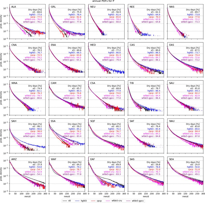
1534                                                                                                  P. Berg et al.: HydroGFD3.0

                                                                       5. Calculate the ratio (for P ) or difference (for T ) between
                                                                          the monthly means of the reference and e5.
                                                                       6. Apply the ratio or difference to all time steps of e5
                                                                          within the month.
                                                                       7. Calculate mean, minimum, and maximum T from the
                                                                          hourly time steps (T only).

                                                                        For P , the scaling can cause very large values in some
                                                                     cases, e.g. when e5 severely underestimates the number
                                                                     of wet days. Therefore, P is limited to a maximum of
                                                                     1500 mm/day, which is close to the highest observed record
                                                                     at that timescale.
Figure 1. Distribution of the absolute difference in the number of
wet days Nwet estimated through the Stillman and Zeng (2016)
method and gpcch P . The probability density function ranges glob-   3.5   Consistency in time and space
ally over all land grid points.
                                                                     To have consistent output in all versions of HydroGFD3,
                                                                     there are internal checks to verify that each of the defined grid
(2016). Note that we do not need to define a wet day using a         points of HydroGFD3 is receiving data after each monthly
specific threshold value. Instead, the number of wet days in a       adjustment. It happens that the land–sea masks of the ob-
month is directly defined by the method. The method essen-           servational data sets change over time, and they often differ
tially relates the number of wet days, Nwet , to the monthly         between different data sources. If the anomaly data are not
P anomaly, Panom , using also the climatological wet-day fre-        defined for a particular grid point, a search algorithm will
quency (calculated from cru wet-day data set), Nwet  clim as a       identify if there are defined anomalies in grid points within a
predictor, and a tunable constant k.                                 five-grid-box radius. If the search is successful in finding at
                                                                     least one value, the mean of all values in the search radius is
        k       clim
Nwet = Panom · Nwet                                           (3)    used to fill the grid point value. However, if no defined data
                                                                     are found, the anomaly will be set to 0 for T and 1 for P ; in
                                                                     other words, the adjustment will be toward the HydroGFD3
   A value of k = 0.28 was derived for HydroGFD2.0 by cal-           climatology.
ibration to the cru observations of the number of wet days in
a month together with the cpcp P observations. This value is
                                                                     3.6   Evaluation
almost half of that found by Stillman and Zeng (2016), which
can probably be related to the data sets used but was found to       Evaluation of the HydroGFD3 historical data set is presented
be highly applicable across the world. A verification of this        for the mean climatology of P and T as well as for regional
constant was performed with the cru wet days and the gpcch           probability distribution functions (PDFs) of daily data and
monthly P anomalies; see Fig. 1. This reveals an overall high        as monthly mean time series. The two latter evaluations are
accuracy of the method, with deviations from observations of         performed for each of the regions defined by Giorgi and Bi
mostly only a few days in a month but which can in rare cases        (2005) (although we use the correct longitude and latitude
be as much as 10 d. On average over the 1980–2009 period             coordinates provided by Huebener and Körper, 2013), com-
and for each single grid point, the deviations are close to 0.       monly referred to as Giorgi regions; see Fig. 2. One exception
Thus, the method works well across all areas and with suffi-         is that we have left out the EQF region in the plots of PDFs
cient precision for our purposes.                                    since it is contained in other included regions. The reason
                                                                     is that it overlaps other regions, and having only 25 regions
3.4    Applied corrections                                           simplifies the presentation layout of the plots substantially.
                                                                     For both the PDFs and the time series, only data points in
The production of the corrected data consists of the following       the defined grid points of HydroGFD3 are used. The PDFs
steps.                                                               are pooling all data in each domain, whereas the time series
  1. Calculate observed anomalies.                                   plots are based on regional averages for each monthly time
                                                                     step.
  2. Construct absolute reference data by adding the anoma-
     lies to the HydroGFD3 climatology.
  3. Calculate the number of wet days (P only).
  4. Remove the weakest excessive wet days in e5 (P only).

Earth Syst. Sci. Data, 13, 1531–1545, 2021                                           https://doi.org/10.5194/essd-13-1531-2021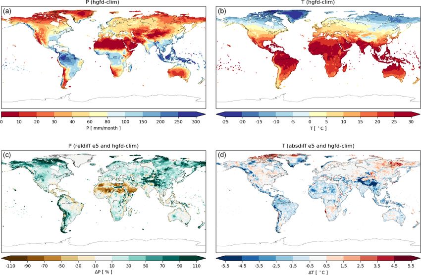
P. Berg et al.: HydroGFD3.0 1535
Figure 2. Evaluation regions as defined by Giorgi and Bi (2005) and employed in the PDF and time series analysis.
4 Data sets Operational aspects
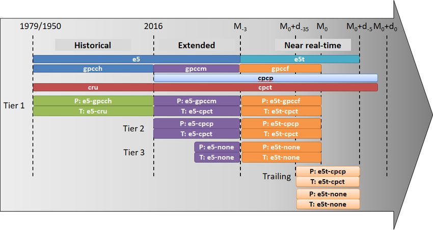
HydroGFD3 is built up by different data sets depending on The HydroGFD3 data sets are updated at regular intervals.
the time period and the tier; see schematic in Fig. 3. The “extended” period is updated each month as new e5 and
The historical period (1979–2016) is built on e5, corrected other data sets become available. Each tier works indepen-
with the gpcch and cru data sets, respectively, for P and T . dently and can therefore become available at different times.
There is only one tier produced for this period; e5 will later The “near-real-time” period is updated at earliest 5 d into
be released back to 1950, and the HydroGFD3 historical data the new month, when e5t is available. By then, the cpcp
will then cover that period as well. and cpct products are generally available, but gpccf normally
After 2016, in the “extended” and “near-real-time” peri- needs a few days more. Tier 3 needs no additional data sets
ods, there are three tiers built on different data sets. Tier 1 is and is available together with e5t but is produced at the cal-
the primary choice and follows the gpccm (for the e5 period) endar month time step like the other products. The priority
and gpccf (for the e5t period) products for P adjustments, order is independent for each variable and goes from Tier
and the cpct product (for the complete period) is used for T . 1–3.
Tier 2 builds instead on the cpcp and cpct products. Note that Finally, the “trailing” updates are performed along with
the Tier 1 and Tier 2 T products are identical and are only e5t and cpcp and cpct updates and is normally available at a
repeated here for simplification of the schematic. In practice, 5 d time lag.
there is no Tier 2 for T , and the tiers are anyway not necessar-
ily used consistently for T and P together since the data sets
5 Results
are completely independent. Tier 3 is the final resort if none
of the data sets for a variable are available. It is performing
5.1 Climatology
only a climatological correction of e5 or e5t by calculating
anomalies of the reanalysis and adding this to or multiplying The climatological period of HydroGFD3 is set to 1980–
it by the HydroGFD3 climatology. Since it does not make 2009 and is consistently used in this section. Figure 4
use of any observational data sets, it has received the internal presents the annual mean climatology of HydroGFD3 for
file naming convention “none”. For P , also the number of both P and T as well as the bias of the e5 reanalysis to this
wet days is adjusted according to the description in Sect. 3.3, climatology; e5 has in general a wet and cold bias in moun-
using the reanalysis anomalies as a predictor. tainous regions in most of the world. The Arctic is gener-
A closer-to-real-time product is possible, with the daily ally wetter and warmer in e5; note that Greenland P is bias-
time step cpcp and cpct products being available with a 2 d free per definition since the HydroGFD3 climatology uses e5
latency and e5t available at 5 d latency. The adjustment of the there. The tropics are generally drier and colder in e5.
e5t data is then based on the latest available 30 d, synchro- Figures S1–S4 show the seasonal HydroGFD3 climatol-
nized between the data sets, and is therefore called “trailing”. ogy and biases of e5. The bias patterns are rather stable
across the seasons, although the magnitude changes some-
what. Most striking are the relative changes in western Africa
in the December–February period, but this is the dry period
https://doi.org/10.5194/essd-13-1531-2021 Earth Syst. Sci. Data, 13, 1531–1545, 2021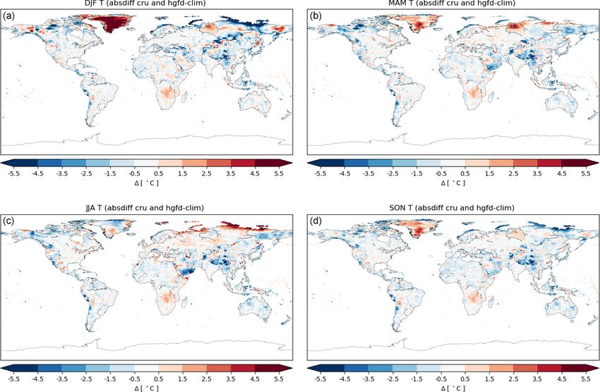
1536                                                                                                           P. Berg et al.: HydroGFD3.0

Figure 3. Schematic of the different HydroGFD3 products on a non-linear time axis. The top bars show the original data sources, and the
Tier 1–3 and trailing products are shown below. Abbreviations follow Table 1. The time axis denotes years with significant changes in data
sources, and the later time marks are relative to the 1st of the current month, M0 , and the current day, d0 . The sub-script for the month is in
months and for the days in days.

Figure 4. The baseline HydroGFD3 annual mean climatology for P (a) and T (b). The bottom row shows the bias of the e5 reanalysis for
each variable to the climatology. Note that the lack of P bias for e5 in Greenland is due to the definition of using e5 climatology for that
region.

Earth Syst. Sci. Data, 13, 1531–1545, 2021                                                   https://doi.org/10.5194/essd-13-1531-2021
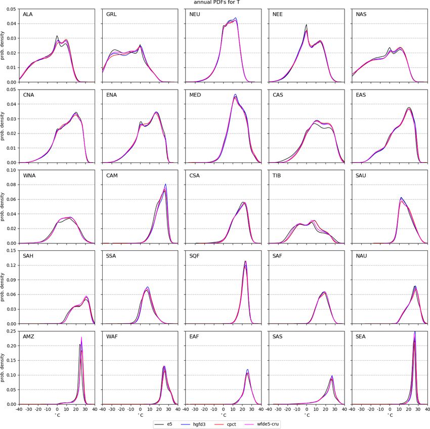
P. Berg et al.: HydroGFD3.0                                                                                                    1537

there, and the relative changes are therefore comparing low        vations used. The use of anomalies from the cru and cpct in
numbers, which tend to exaggerate the absolute term differ-        constructing the final data set removes such effects, but the
ences.                                                             climatological difference remains.
   We also compare the HydroGFD3 climatologies to other
data sets, mainly with a focus on data with daily time steps       5.2   Distributions
that could be used equally for the historical period but also to
gpcch, which is the main background data set for anomalies         Figure 7 shows the PDFs for the complete time period 1980–
in the historical period. Figure 5 shows the annual mean dif-      2009 for P and for each of the data sets e5, hgfd3, cpcp,
ference in P of gpcch, cpcp, wfde5-gpcc, and wfde5-cru to          wfde5-cru, and wfde5-gpcc. In these plots, the spread be-
the HydroGFD3 climatology. Differences to gpcch are gen-           tween the coloured lines representing direct observations or
erally within ±10 %, except for parts of the Andes moun-           e5 adjusted to observations can be interpreted as indicators
tain range, the Canadian Arctic, the dry north of Africa, the      of the uncertainty in the observed state. Many regions show
Himalayan plateau, and Greenland. These are all dry and/or         fairly high agreement between the data sets, including the
snowy regions, with an inherent observational uncertainty,         original e5 data. In some regions, there is a large spread in
adding the lower gauge network density in the areas. The           the observations, and e5 is somewhere in between, e.g. in
presented differences between the data sets are considered         ALA, GRL, TIB, and SAH. Again, these regions have large
well inside this expected uncertainty range. We also remark        observational uncertainty, making it difficult to determine a
that uncertainties in Greenland are especially large due to        ground truth. However, in other regions e5 is deviating sig-
few observations and difficult conditions, and data for this       nificantly in part of the distribution, such as in SSA and WAF
region should be used carefully with HydroGFD3 and other           moderate intensities and AMZ and EAF extreme intensities.
data sets alike. The cpcp data set is generally drier, espe-          HydroGFD3 tends to have higher extremes than other data
cially in the Arabian Peninsula; wfde5-gpcc and wfde5-cru          sets. This is partly a resolution effect due to the 0.25◦ resolu-
are both generally wetter than the HydroGFD3 climatology,          tion of HydroGFD3 and 0.5◦ of the other data sets used here.
especially in the cold seasons (see Fig. S5–S8). This is due       A coarser resolution will move all higher intensities toward
to the gauge corrections applied in the wfde5 data, which is       the lower intensities (to the left in the PDF plots). That the ef-
also the reason for wfde5-gpcc not being identical to gpcch,       fect differs between regions is because the extremes are also
which it is based on. There are also discrepancies in large        modulated by the magnitude of the applied correction, i.e.
dry desert areas such as the Sahara desert, which arise due to     the applied scaling. A scaling factor above 1 will increase the
differences in the way the number of wet days is calculated        extremes and below 1 will decrease them. The baseline cli-
in the different data sets. The WFDE5 implementation would         matology therefore has an impact on the extremes. Also the
produce NaN (not a number) in division by 0 if the number          wet-day calculation of HydroGFD3 can affect the results, and
of wet days was 0, which has not happened so far (reviewer         we find that the dry regions, e.g. SAH and MED, have more
comment by Graham Weedon). In HydroGFD3, division by               dry days in HydroGFD3 than in the other data sets. When e5
0 does occur and is solved by setting the ratio to 0 when the      only gives few P days, while the observational anomaly is
calculated number of dry days equals 0. An incompatibility         high, the scaling factor can become very large, and the only
between P and no observed wet days can act to remove P             process to limit this is the upper limit of 1500 mm/d, which
completely for some months, therefore making a drier data          is seldom reached. The wfde5-gpcc, which has a similar
set. Seasonal differences (Fig. S5–S8) show similar patterns       methodology as HydroGFD3, still has lower extremes. Be-
as the annual mean for most of the regions but can also differ     sides the above-mentioned undercatch corrections, the lower
substantially in some regions. One region that stands out is       extremes may be due to the upper threshold applied to each
southern Africa in June–August, where both gpcch and cpcp          hour, as can be seen in the original wfde5 code in the CDS
show much wetter conditions (Fig. S7).                             (Climate Data Store) catalogue (Copernicus Climate Change
   For T , we compare to cru only since cpct is used to build      Service , 2020a).
the climatology on top of which cru anomalies are added,              For T , the general shapes of the PDFs agree across all
and wfde5-cru is adjusted to cru and is per definition identi-     data sets and regions (Fig. 8). However, there are some-
cal regarding climatology. Figure 6 shows the absolute differ-     times substantial differences between e5 and the observa-
ence in cru and the HydroGFD3 climatology for each season          tional data sets. Typically, e5 displays issues around 0 ◦ C,
of the climatological year. The largest differences are in the     which is common in global models and related to melting
Arctic region, where gauge availability is low. In other re-       conditions. There are also seasonal offsets outside the range
gions, such as south-central Africa, the Himalayan plateau,        of the observations. HydroGFD3 remains fairly close to cpct
and other orographic regions, the differences are very con-        and wfde5-cru in most cases. Orographic effects on T were
sistent over all seasons, with deviations up to a few degrees      not accounted for in this comparison, which can explain
Celsius. This makes us suspect that they are due to differ-        some of the differences in regions with varying orography
ences in the elevation used for the different data sets. The       such as TIB.
cpct data set does not come with any information on the ele-

https://doi.org/10.5194/essd-13-1531-2021                                          Earth Syst. Sci. Data, 13, 1531–1545, 2021
1538 P. Berg et al.: HydroGFD3.0
Figure 5. Relative difference in data sets to the HydroGFD3 annual mean P climatology for the period 1980–2009; gpcch (a), cpcp (b),
wfde5-gpcc (c), and wfde5-cru (d).
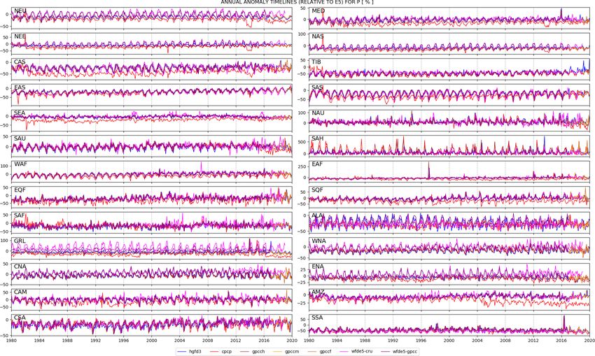
5.3 Temporal trends other data sets. This is likely due to the undercatch correc-
tions, which are larger for snowy conditions. As expected,
HydroGFD3 follows the general trends of wfde5-gpcc, and
To get an impression of the temporal trends and to identify
the other data sets have similar trends besides the cpcp devia-
potential issues in the time series, we also investigate the time
tions just discussed. The gpccm and gpccf have similar mean
series as an average over the Giorgi regions. To emphasize
and variance as gpcch in the overlapping period and show
differences between the data sets, we discuss mainly differ-
generally consistent behaviour for the later years. However,
ences relative to a common reference, here chosen to be e5.
some larger anomalies occur in, for example, CAN, CAM,
In other words, we present the inverse bias of e5 compared
SQF, and SAH.
to each observational source.
For T , the anomalies to e5 (see Fig. 10 and Fig. S10) retain
Figure 9 shows the results for P for the period 1980–
a clear annual cycle in many regions. Sometimes, the annual
2019, and the absolute values are shown in Fig. S9. Note
cycle is mainly for wfde5-cru (e.g, NEU, TIB, SAS) but often
that wfde5-gpcc ends in 2016, wfde5-cru ends in 2018, and
for all data sets. HydroGFD3 and cpct are in general close to
gpccm and gpccfg are only available for the last years. The
each other because of the HydroGFD3 climatology reducing
most striking feature is the strong deviations in cpcp for
the offset to 0. However, cpct has some clear “break points”
many of the regions. It also varies significantly with time by
in its time series in some regions. For example, in NEU, there
changing variance, e.g. in SEA, changing mean value, e.g.
is a marked change in the magnitude of the anomalies from
in CAS, SAS, and AMZ. In some years, there are significant
about 0 to 0.5 ◦ C to −0.5 to 0.5 ◦ C in about 2006. A sim-
offsets compared to surrounding years, e.g. in 2014 in NEU,
ilar change about that time is visible also for EAS, GRL,
NEE, CAS, and MED. Likely, these issues are due to varia-
MED, SAS, and NAU. Because the climatologies are cal-
tions in the underlying station network, but we have not ver-
culated for the period 1980–2009, part of these changes are
ified this. All data sets show signs of an annual cycle in their
included with the earlier weaker variability. HydroGFD3 is
anomalies to e5 in colder regions, which is indicative of dif-
based on cru anomalies pre-2016, but from 2016 on, also its
ferences between warm- and cold-season precipitation. The
variability is subjected to the changes in cpct.
wfde5-gpcc and wfde5-cru data sets display stronger anoma-
lies over the annual cycle in the colder regions compared to
Earth Syst. Sci. Data, 13, 1531–1545, 2021 https://doi.org/10.5194/essd-13-1531-2021P. Berg et al.: HydroGFD3.0 1539
Figure 6. Absolute-difference T climatology for the period 1980–2009 between cru and HydroGFD3 for each season: (a) December–
February, (b) March–May, (c) June–August, and (d) September–November.
Some regions display a significant offset between the data 6 Discussion
sets, such as SEA, CSA, MED, TIB, and SAS, with cru hav-
ing generally lower T values. Interestingly, changes in cpct
Compared to similar data sets based on reanalysis, such as
after 2006 often act to reduce the offset to e5.
WFDE5 and MSWEP, HydroGFD3 differs in that it has its
own climatological background and performs the corrections
5.4 Extending to near real time based on anomalies of that same climatological time period.
The near-real-time products, in Fig. 3 called “trailing”, use The reason for using this method is to be able to switch data
the daily updates of the cpcp and cpct observations. They are sets closer to real time without “jumps” in the time series.
therefore subject to the quality of the cpcp and cpct prod- This works well as long as the real-time data set retains its
ucts and the changes in time as discussed in the previous climatological state, which seems to be the case for gpccm
section. This product follows HydroGFD3 fairly closely to and gpccf compared to gpcch. However, cpct and cpcp both
that shown in Figs. 9 and 10 as the main-version Tier 2 is cause issues due to changes in the time series towards the
also based on cpcp and cpct but with corrections at calendar end of the time period, in about 2006. The bias of e5 is still
months. reduced, which brings validity to the method. A future de-
In addition, also the “none” products are created with the velopment could be to instead retain trends from the ERA5
trailing time window. These only replace the e5 climatology reanalysis and explore the use of shorter periods for calculat-
with that of HydroGFD3 and are the simplest form of correc- ing anomalies of the observed data. This would reduce dis-
tions of the mean. They act as the last failsafe option in the continuities in the time series but would remove the potential
production chain before defaulting to uncorrected e5 data. benefits of using trends from the observations.
We do not present this product in the time series plots since it HydroGFD3 has generally higher extremes than the other
would only constitute a constant annual cycle offset in com- analysed data sets. This is especially so in drier regions
parison to e5. where an interplay between the estimation of the number of
wet days and the scaling causes fewer wet days and larger
scaling factors. In effect, this leads to enlarging the tail of the
distribution, e.g. in the MED and SAH region in Fig. 7. It is
https://doi.org/10.5194/essd-13-1531-2021 Earth Syst. Sci. Data, 13, 1531–1545, 20211540 P. Berg et al.: HydroGFD3.0 Figure 7. P PDFs of each Giorgi region for the data sets with daily output data in the period 1980–2009. The table in each plot states the percentage of dry days for each data set, i.e. the percentage of data in the first bin of 0–1 mm/d. possible to restrict the scaling by only allowing the scaling in regions where data are not generally available to all data factor to be a few times the original value, but such restric- sets. It is therefore difficult to determine which is closer to tions would in turn impact the monthly mean. A potential the truth in a global assessment like this, and more detailed method would be to “borrow” P from adjacent grid points regional studies, such as Fallah et al. (2020), are needed. on e5’s excessive dry days, thereby reducing the scaling fac- The current main usage of the data set is to initialize dif- tors. This topic is being investigated for future updates of the ferent HYPE forecasting models around the world, e.g. in methodology. Europe (Hundecha et al., 2016), the Niger River (Andersson The regional analysis shows clearly that the observational et al., 2017), and worldwide (Arheimer et al., 2020). This has data sets give substantially different results in some regions. influenced some of the choices for the set-up, such as the use Diverse results are more common in data-sparse regions or of only the ERA5 reanalysis model, among other reanalysis Earth Syst. Sci. Data, 13, 1531–1545, 2021 https://doi.org/10.5194/essd-13-1531-2021
P. Berg et al.: HydroGFD3.0                                                                                                   1541

Figure 8. T PDFs of each Giorgi region for the data sets with daily output data in the period 1980–2009.

systems used in e.g. the MSWEP data set (Beck et al., 2017).           7   Data availability
The forecasts produced by these hydrological models are pri-
marily using the ECMWF deterministic medium-range fore-                For HydroGFD3, a historical period, ranging from
casts or the probabilistic SEAS5 seasonal forecasts, which             February 1979 to December 2019, is available
both use the same model as e5. The priority order of the dif-          as open source from the Zenodo repository at
ferent redundancy options, i.e. the Tiers 1–3, is based on ex-         https://doi.org/10.5281/zenodo.3871707 (Berg et al.,
perience with using the different data sources for our fore-           2020). For years prior to 2017, cru and gpccm are used as
casts, with impact from both availability for a given month            reference data for T and P , respectively. The following
and experienced longer interruptions.                                  years use instead cpct and gpccm reference data. Real-time
                                                                       updates of the data set are available for a processing charge
                                                                       via subscriptions. Please make a request here at https:

https://doi.org/10.5194/essd-13-1531-2021                                               Earth Syst. Sci. Data, 13, 1531–1545, 2021
1542 P. Berg et al.: HydroGFD3.0 Figure 9. Monthly P anomalies for all data sets, averaged over the Giorgi regions for all valid land data points. The anomalies are relative to the e5 data set and are evaluated for each single month. Earth Syst. Sci. Data, 13, 1531–1545, 2021 https://doi.org/10.5194/essd-13-1531-2021
P. Berg et al.: HydroGFD3.0                                                                                                            1543

Figure 10. Monthly T anomalies for all data sets, averaged over the Giorgi regions for all valid land data points. The anomalies are relative
to the e5 data set and are evaluated for each single month.

https://doi.org/10.5194/essd-13-1531-2021                                                Earth Syst. Sci. Data, 13, 1531–1545, 2021
1544                                                                                                     P. Berg et al.: HydroGFD3.0

//hypeweb.smhi.se/buy-water-services/data-subscription/             Arheimer, B., Pimentel, R., Isberg, K., Crochemore, L., Anders-
(last access: 22 March 2021) and make sure to mention the              son, J. C. M., Hasan, A., and Pineda, L.: Global catchment mod-
data set name “HydroGFD3”. All data sets listed in Table 1             elling using World-Wide HYPE (WWH), open data, and step-
are available through the provided references.                         wise parameter estimation, Hydrol. Earth Syst. Sci., 24, 535–
                                                                       559, https://doi.org/10.5194/hess-24-535-2020, 2020.
                                                                    Ashouri, H., Hsu, K.-L., Sorooshian, S., Braithwaite, D. K., Knapp,
8    Conclusions                                                       K. R., Cecil, L. D., Nelson, B. R., and Prat, O. P.: PERSIANN-
                                                                       CDR: Daily Precipitation Climate Data Record from Multisatel-
The HydroGFD3 methodology of correcting the e5 reanaly-                lite Observations for Hydrological and Climate Studies, B. Am.
sis model toward an observational reference, along with the            Meteorol. Soc., 96, 69–83, https://doi.org/10.1175/bams-d-13-
resulting data sets, was presented. We conclude that the data          00068.1, 2015.
sets compare well with existing similar data sets.                  Beck, H. E., van Dijk, A. I. J. M., Levizzani, V., Schellekens,
   The main new features of HydroGFD3 are                              J., Miralles, D. G., Martens, B., and de Roo, A.: MSWEP: 3-
                                                                       hourly 0.25° global gridded precipitation (1979–2015) by merg-
    – higher spatial resolution of 0.25◦                               ing gauge, satellite, and reanalysis data, Hydrol. Earth Syst. Sci.,
                                                                       21, 589–615, https://doi.org/10.5194/hess-21-589-2017, 2017.
    – near-real-time corrected data until 5 d from now, i.e. fol-   Berg, P., Donnelly, C., and Gustafsson, D.: Near-real-time adjusted
      lowing the continuously updated e5 + e5t time period             reanalysis forcing data for hydrology, Hydrol. Earth Syst. Sci.,
                                                                       22, 989–1000, https://doi.org/10.5194/hess-22-989-2018, 2018.
    – temporal coverage from 1979, which will be extended           Berg, P., Almén, F., and Bozhinova, D.: HydroGFD3.0, Zenodo,
      back to 1950 along with the extended e5 data expected            https://doi.org/10.5281/ZENODO.3871707, 2020.
      during 2021                                                   C3S (Copernicus Climate Change Service): Near surface meteoro-
                                                                       logical variables from 1979 to 2018 derived from bias-corrected
    – multiple redundancy options to avoid halting production          reanalysis, https://doi.org/10.24381/cds.20d54e34, 2020.
      when single data sets are delayed.                            C3S      (Copernicus      Climate      Change       Service):      ERA5
                                                                       hourly data on single levels from 1979 to present,
                                                                       https://doi.org/10.24381/cds.adbb2d47, 2020.
                                                                    Chen, M., Shi, W., Xie, P., Silva, V. B. S., Kousky, V. E.,
Supplement. The supplement related to this article is available
                                                                       Wayne Higgins, R., and Janowiak, J. E.: Assessing ob-
online at: https://doi.org/10.5194/essd-13-1531-2021-supplement.
                                                                       jective techniques for gauge-based analyses of global
                                                                       daily precipitation, J. Geophys. Res.-Atmos., 113, D04110,
                                                                       https://doi.org/10.1029/2007JD009132, 2008.
Author contributions. PB developed the methodology and de-          CHP (Climate Hazards Group): Monthly quasi-global satellite
signed the experiments. FA developed the code and infrastructure       and observation based precipitation climatology, available at:
for the operational system. DB performed analysis and prepared         https://data.chc.ucsb.edu/products/CHPclim/netcdf/ (last access:
figures for the manuscript. PB prepared the manuscript with con-       18 September 2020), 2015.
tributions from all co-authors.                                     Climate Hazards Group (CHP): Monthly quasi-global satellite
                                                                       and observation based precipitation climatology, available at:
                                                                       https://data.chc.ucsb.edu/products/CHPclim/netcdf/ (18 Septem-
Competing interests. The authors declare that they have no con-        ber 2020), 2015.
flict of interest.                                                  Climate Prediction Center (CPC): CPC Unified gauge-based analy-
                                                                       sis of global daily precipitation, available at: https://ftp.cpc.ncep.
                                                                       noaa.gov/precip/CPC_UNI_PRCP/GAUGE_GLB/ (18 Septem-
Acknowledgements. The authors would like to thank the EU and           ber 2020), 2021.
the Swedish Research Council Formas for funding within the frame-   Copernicus Climate Change Service (C3S): Near surface meteoro-
work of the GlobalHydroPressure project, financed under the 2017       logical variables from 1979 to 2018 derived from bias-corrected
Joint Call of Water JPI (IC4WATER).                                    reanalysis, https://doi.org/10.24381/cds.20d54e34, 2020a.
                                                                    Copernicus Climate Change Service (C3S): ERA5 hourly
                                                                       data on single levels from 1979 to present [dataset],
Review statement. This paper was edited by Martin Schultz and          https://doi.org/10.24381/cds.adbb2d47, 2020b.
reviewed by Graham Weedon and one anonymous referee.                CPC (Climate Prediction Center): https://www.esrl.noaa.gov/psd/
                                                                       data/gridded/data.cpc.globaltemp.html (last access: 18 Septem-
                                                                       ber 2020), 2017.
                                                                    CPC (Climate Prediction Center): CPC Unified gauge-based analy-
References                                                             sis of global daily precipitation, available at: https://ftp.cpc.ncep.
                                                                       noaa.gov/precip/CPC_UNI_PRCP/GAUGE_GLB/ (last access:
Andersson, J. C., Ali, A., Arheimer, B., Gustafsson, D., and Mi-       18 September 2020), 2020.
  noungou, B.: Providing peak river flow statistics and forecast-   CPCtemp: https://www.esrl.noaa.gov/psd/data/gridded/data.cpc.
  ing in the Niger River basin, Phys. Chem. Earth, 100, 3–12,          globaltemp.html (last access: 18 September 2020), 2017.
  https://doi.org/10.1016/j.pce.2017.02.010, 2017.

Earth Syst. Sci. Data, 13, 1531–1545, 2021                                            https://doi.org/10.5194/essd-13-1531-2021
P. Berg et al.: HydroGFD3.0 1545 Cucchi, M., Weedon, G. P., Amici, A., Bellouin, N., Lange, S., Hundecha, Y., Arheimer, B., Donnelly, C., and Pechlivanidis, I.: Müller Schmied, H., Hersbach, H., and Buontempo, C.: WFDE5: A regional parameter estimation scheme for a pan-European bias-adjusted ERA5 reanalysis data for impact studies, Earth multi-basin model, J. Hydrol. Regional Studies, 6, 90–111, Syst. Sci. Data, 12, 2097–2120, https://doi.org/10.5194/essd-12- https://doi.org/10.1016/j.ejrh.2016.04.002, 2016. 2097-2020, 2020. Joyce, R. J., Janowiak, J. E., Arkin, P. A., and Xie, P.: Fallah, A., Rakhshandehroo, G. R., Berg, P. O. S., and Orth, CMORPH: A Method that Produces Global Precipita- R.: Evaluation of precipitation datasets against local observa- tion Estimates from Passive Microwave and Infrared tions in southwestern Iran, Int. J. Climatol., 40, 4102–4116, Data at High Spatial and Temporal Resolution, J. Hy- https://doi.org/10.1002/joc.6445, 2020. drometeorol., 5, 487–503, https://doi.org/10.1175/1525- Fan, Y. and Van den Dool, H.: A global monthly land surface air 7541(2004)0052.0.co;2, 2004. temperature analysis for 1948–present, J. Geophys. Res.-Atmos., Lindström, G., Pers, C., Rosberg, R., Strömqvist, J., and Arheimer, 113, D01103, https://doi.org/10.1029/2007JD008470, 2008. B.: Development and test of the HYPE (Hydrological Pre- Funk, C., Peterson, P., Landsfeld, M., Pedreros, D., Verdin, J., dictions for the Environment) model – A water quality Shukla, S., Husak, G., Rowland, J., Harrison, L., Hoell, A., and model for different spatial scales, Hydrol. Res., 41, 295–319, Michaelsen, J.: The climate hazards infrared precipitation with https://doi.org/10.2166/nh.2010.007, 2010. stations – a new environmental record for monitoring extremes, Schneider, U., Becker, A., Finger, P., Meyer-Christoffer, Sci. Data, 2, 150066, https://doi.org/10.1038/sdata.2015.66, A., and Ziese, M.: GPCC Full Data Monthly Ver- 2015a. sion 2018.0 at 0.25: Monthly Land-Surface Precipita- Funk, C., Verdin, A., Michaelsen, J., Peterson, P., Pedreros, D., and tion from Rain-Gauges built on GTS-based and His- Husak, G.: A global satellite-assisted precipitation climatology, toric Data, Global Precipitation Climatology Centre, Earth Syst. Sci. Data, 7, 275–287, https://doi.org/10.5194/essd- https://doi.org/10.5676/DWD_GPCC/FD_M_V2018_025, 7-275-2015, 2015b. 2018a. Giorgi, F. and Bi, X.: Updated regional precipitation and tem- Schneider, U., Becker, A., Finger, P., Meyer-Christoffer, A., perature changes for the 21st century from ensembles of re- and Ziese, M.: GPCC Monitoring Product Version 6.0 cent AOGCM simulations, Geophys. Res. Lett., 32, L21715, at 1.0: Near Real-Time Monthly Land-Surface Precip- https://doi.org/10.1029/2005gl024288, 2005. itation from Rain-Gauges based on SYNOP and CLI- Harris, I. C. and Jones, P. D.: CRU TS4.03: Climatic Re- MAT Data, Global Precipitation Climatology Centre, search Unit (CRU) Time-Series (TS) version 4.03 of https://doi.org/10.5676/DWD_GPCC/MP_M_V6_100, 2018b. high-resolution gridded data of month-by-month varia- Stillman, S. and Zeng, X.: Development of a 0.5◦ global monthly tion in climate (Jan. 1901–Dec. 2018), CEDA Archive, raining day product from 1901 to 2010, Geophys. Res. Lett., 43, https://doi.org/10.5285/10D3E3640F004C578403419AAC167D82, 9704–9711, https://doi.org/10.1002/2016gl070244, 2016. 2019. Weedon, G., Gomes, S., Viterbo, P., Shuttleworth, W., Blyth, E., Hersbach, H., Bell, B., Berrisford, P., Hirahara, S., Horányi, A., Österle, H., Adam, C., Bellouin, N., Boucher, O., and Best, Muñoz-Sabater, J., Nicolas, J., Peubey, C., Radu, R., Schep- M.: Creation of the watch forcing data and its use to as- ers, D., Simmons, A., Soci, C., Abdalla, S., Abellan, X., Bal- sess global and regional reference crop evaporation over land samo, G., Bechtold, P., Biavati, G., Bidlot, J., Bonavita, M., during the twentieth century, J. Hydrometeor., 12, 823–848, Chiara, G., Dahlgren, P., Dee, D., Diamantakis, M., Dragani, R., https://doi.org/10.1175/2011JHM1369.1, 2011. Flemming, J., Forbes, R., Fuentes, M., Geer, A., Haimberger, Weedon, G. P., Balsamo, G., Bellouin, N., Gomes, S., Best, M. J., L., Healy, S., Hogan, R. J., Hólm, E., Janisková, M., Keeley, and Viterbo, P.: The WFDEI meteorological forcing data set: S., Laloyaux, P., Lopez, P., Lupu, C., Radnoti, G., Rosnay, P., WATCH Forcing Data methodology applied to ERA-Interim re- Rozum, I., Vamborg, F., Villaume, S., and Thépaut, J.-N.: The analysis data, Water Resour. Res., 50, 7505–7514, 2014. ERA5 global reanalysis, Q. J. Roy. Meteor. Soc., 146, 1999– 2049, https://doi.org/10.1002/qj.3803, 2020. Huebener, H. and Körper, J.: Changes in Regional Potential Vege- tation in Response to an Ambitious Mitigation Scenario, J. En- viron. Prot., 4, 16–26, https://doi.org/10.4236/jep.2013.48a2003, 2013. https://doi.org/10.5194/essd-13-1531-2021 Earth Syst. Sci. Data, 13, 1531–1545, 2021
You can also read