Trade Policy Uncertainty and Stock Returns
←
→
Page content transcription
If your browser does not render page correctly, please read the page content below
Munich Personal RePEc Archive

Trade Policy Uncertainty and Stock
Returns

Esposito, Federico and Bianconi, Marcelo and Sammon,
Marco

Tufts University

2 April 2020

Online at https://mpra.ub.uni-muenchen.de/99874/
MPRA Paper No. 99874, posted 29 Apr 2020 07:26 UTC
Trade Policy Uncertainty and Stock Returns∗
          Marcelo Bianconi                 Federico Esposito               Marco Sammon
                   Tufts                           Tufts                         Kellogg

                                              April 2020

                                                Abstract

       We examine how trade policy uncertainty is reflected in stock returns. Our identification
       strategy exploits quasi-experimental variation in exposure to trade policy uncertainty
       arising from Congressional votes to revoke China’s preferential tariff treatment between
       1990 and 2001. More exposed industries commanded a risk premium of 6% per year.
       The risk premium was larger in sectors less protected from globalization, and more
       reliant on inputs from China. More exposed industries also had a larger drop in stock
       prices when the uncertainty began, and more volatile returns around key policy dates.
       Moreover, the effects of policy uncertainty on expected cash-flows, investors’ forecast
       errors, and import competition from China cannot explain our results.

   ∗
    Bianconi:       Tufts University, 8 Upper Campus Road, Medford, MA 02155 (e-mail:
marcelo.bianconi@tufts.edu); Esposito: Tufts University, 8 Upper Campus Road, Medford, MA
02155 (e-mail: federico.esposito@tufts.edu); Sammon: Northwestern University, Kellogg School of
Management, Evanston, IL 60201 (e-mail: mcsammon@gmail.com). We thank Erik Loualiche for providing us
the globalization factor data. We thank Scott Baker, Steve Davis, Ian Dew-Becker, Jose Fillat, Craig Furfine,
Abigail Hornstein, Ravi Jagannathan, Cynthia Kinnan, Robert Korajczyk, Margaret McMillan, Dimitris
Papanikolaou, Peter Schott, Martin Thyrsgaard, and numerous seminar participants at Northwestern,
Midwest Trade Conference at Vanderbilt, Tufts University, London School of Economics, Atlanta Fed, ASSA
2020, MIT Sloan, for helpful suggestions.
1 Introduction
The recent threat of a trade war between US and China has brought trade policy uncertainty
(henceforth TPU) to the forefront of the economic and policy debate. A growing empirical
literature has analyzed the effects of TPU on employment (see e.g. Pierce and Schott (2016)),
trade (see Alessandria et al. (2019), Crowley et al. (2018), Graziano et al. (2018)), investment
(see Handley and Limão (2015), Pierce and Schott (2017), Caldara et al. (2020)), and welfare
(see Handley and Limão (2017) and Steinberg (2019)). While this literature has focused on
the impact of TPU on economic outcomes, it has remained silent on its effect on asset prices.
Given the relevance that stock prices have for firms’ investment decisions (see e.g. Chen et al.
(2006)), household wealth (see e.g. Guiso et al. (2002), Moskowitz and Vissing-Jørgensen
(2002)), and employment (see e.g. Chodorow-Reich et al. (2019)), studying how financial
markets respond to policy uncertainty deserves further scrutiny.
This paper documents that TPU is a systematic risk factor that affects asset prices. We
capture industries’ exogenous and heterogeneous exposure to TPU arising from Congressional
votes to revoke China’s preferential tariff rates between 1990 and 2001, before China’s
accession to the World Trade Organization (WTO). Empirically, we find a large risk premium
associated with exposure to TPU: investors required an additional 6% return per year on
average as compensation for uncertainty about future trade policy. Moreover, the risk
premium was larger in sectors more exposed to globalization and more reliant on inputs from
China.
We focus on the uncertainty arising from annual votes by Congress to revoke China’s
‘‘Most Favored Nation’’ (MFN) status between 1990 and 2001. Starting in 1980, US imports
from China were subject to Normal Trade Relations (NTR), or equivalently MFN, tariff
rates reserved for WTO members, even though China was not a member of the WTO. This
required annual renewals by Congress, which were essentially automatic until the Tiananmen
Square Massacre in 1989. Starting in 1990, NTR renewal in Congress became more politically
contentious, with the House passing resolutions against Chinese NTR renewal in 1990, 1991
and 1992. China’s tariff status, however, did not change because the US Senate did not
pass the House resolutions. Had NTR status been revoked, tariffs would have reverted to
non-NTR rates, established under the Smoot-Hawley Tariff Act of 1930, which were on
average 27% higher than existing tariffs. The uncertainty about tariff increases on Chinese
goods ended on 12/11/2001, when China joined the WTO, eliminating the need for annual
renewal votes.
We follow Pierce and Schott (2016), and quantify the heterogeneous exposure to policy
uncertainty via the “NTR gap,” defined as the difference between the non-NTR rates, to
1which tariffs would have risen if annual renewal had failed, and the NTR rates. We exploit
the large cross-sectional variation in the NTR gaps across US tradeable sectors and estimate
a differences-in-differences specification in which we regress monthly value-weighted industry
stock returns, between 1980 and 2007, on the industry-level NTR gap, interacted with a
dummy for the period of trade policy uncertainty (hereafter TPU period). The identification
rests on the fact that most of the cross-sectional variation in the NTR gaps comes from
variation in non-NTR rates, set by the Smoot-Hawley Act in 1930, which are likely exogenous
to the US industries’ stock returns 70 years after they were set.
Our baseline results suggest that US tradeable industries more exposed to tariff uncer-
tainty, i.e. industries that had a higher gap between non-NTR and NTR rates, experienced
significantly higher stock returns than less exposed industries between 1990 and 2001. Our
specification controls for unobserved industry- and time-specific characteristics, for industry-
time variation in firm fundamentals, and other contemporaneous US-China policy changes,
such as the global Multi-Fiber Arrangement (MFA) and the reduction in Chinese import
tariffs associated with China’s accession to WTO. The difference in average returns for high
and low NTR gap industries is significant at the 1% level, and implies that going from an
industry less exposed to TPU (at the 25th percentile of the distribution of NTR gaps in
1990), to an industry more exposed (at the 75th percentile of the distribution), increases stock
returns by 4.2% per year during the uncertainty period. When we estimate a dynamic version
of our baseline regression, we find that the correlation between the NTR gap and stock returns
was larger in the early 1990s. This is consistent with greater uncertainty about China’s NTR
status between 1990 and 1992, because this is when the House of Representatives passed a
resolution revoking China’s preferential tariff treatment.
We then argue that the higher average returns earned by more exposed sectors can
be explained by a risk premium for exposure to TPU. Intuitively, during the TPU period,
investors required additional compensation to hold stocks with exposure to this policy
uncertainty, as argued in the theoretical frameworks of Pastor and Veronesi (2012) and
Pástor and Veronesi (2013). Using the predictions of these models to guide our empirical
analysis, we document several stylized facts in support of the risk premium hypothesis.
First, we show that a value-weighted portfolio, long high-gap industries and short low-gap
industries, had average excess returns of 6% per year, over the 5 factors in Fama and French
(2015), during the uncertainty period 1990-2001. Our long-short portfolio’s excess return
remains economically large and statistically significant after controlling for the globalization
factor constructed in Barrot et al. (2018), which uses industry-level shipping costs to proxy
for exposure to globalization. This means that TPU was a systematic factor that could not
be diversified away and could not be explained by exposure to globalization. In addition,
2when we repeat the portfolio analysis in the control periods 1980-1989 and 2002-2007, we
find no significant difference in stock returns between high and low NTR gap industries.
Second, we investigate which, among the high-gap industries, were earning the risk
premium. First, we double sort portfolios on the NTR gap in 1990 and on NTR tariff
rates. The risk premium was concentrated in industries whose exposure to globalization, as
measured by low NTR tariff rates, was higher. We find similar results when we double sort
portfolios on the NTR gap and on industry-level shipping costs from Barrot et al. (2018).
This suggests that exposure to globalization amplifies the effects of trade policy uncertainty
and thus the associated risk premium. An additional amplification channel is the share of
inputs sourced from China: the risk premium was larger among firms with a higher share of
inputs expenditures from China, suggesting that uncertainty about the cost of production
was also priced by financial markets.1
Third, we document a large and significant drop in stock prices for industries with higher
NTR gaps around the day in which the policy uncertainty reasonably began, i.e. the day
when the first resolution to revoke NTR status was proposed at the House, on 07/23/1990.
This is consistent with an increase in the discount rate due to higher uncertainty on future
policies that depressed prices of more exposed industries, as in Pastor and Veronesi (2012).
Fourth, we document that more exposed industries had significantly higher realized
volatility around relevant policy-related events, such as the Congressional votes to revoke
NTR status to China and the day Permanent Normal Trade Relations (PNTR) was granted,
consistent with the evidence shown, in other contexts, in Boutchkova et al. (2012) and Baker
et al. (2019).
To lend further support to our risk premium hypothesis, we discuss three other potential
explanations for our results and show that they are not supported in the data. First, it could
be that the differential returns of high and low NTR gap industries may have been driven
by stock prices’ responses to changes in expected cash-flows, instead of changes in the risk
premium. We repeat the portfolio analysis, but exclude a 3-day window around the dates of
NTR-related policy announcements, as well as Congressional votes to revoke China’s NTR
status. We find that removing these days has a negligible effect on the estimated risk premium.
Second, it could be that investors initially under- or over-estimated the effect of TPU on
firms’ performance. If this were true, we would expect to find large stock-market responses
around the dates US firms released fundamental information in their quarterly earnings
announcements. Empirically, there is no evidence of systematic differences in earnings
1
On this respect, we contribute to the literature that shows the importance of input-output linkages for
economic outcomes (see e.g. Caliendo and Parro (2014), Wang et al. (2018), Adao et al. (2019) and Blaum
et al. (2020)), and for stock returns (see e.g. Cohen and Frazzini (2008) and Huang et al. (2018)).
3announcement returns for stocks with low and high NTR gaps. A third explanation for our
results could be that more uncertainty about future tariffs offered an implicit protection
against Chinese competition for firms in high-gap industries, which, as a result, enjoyed
higher cash flows and higher stock returns during the 1990-2001 period. We test for this
channel by double sorting portfolios on NTR gap and import penetration from China, and
find that, instead, the risk premium was earned by industries more exposed to China.
Our paper is complementary to the empirical literature that investigates the effects of
trade policy uncertainty, and uncertainty in general, on economic outcomes, such as Novy
and Taylor (2014), Pierce and Schott (2016), Handley and Limão (2017), Crowley et al.
(2018) and Esposito (2019). Differently from this literature, we focus on how TPU affects the
riskiness perceived by investors, tracing down its effects on firms’ stock returns. Stock returns
are an important determinant of real economic variables, such as investment (see Chen et al.
(2006)), household wealth (see Guiso et al. (2002)), employment (see Chodorow-Reich et al.
(2019)) and business cycles (see Jordà et al. (2019)), and thus their large and heterogenous
response to TPU, documented in this paper, may have exacerbated the effects of TPU on
economic outcomes.
There is an extensive literature that attempts to empirically assess how policy uncertainty
is priced into stocks and options (see e.g. Pastor and Veronesi (2012), Pástor and Veronesi
(2013), Brogaard and Detzel (2015), Kelly et al. (2016), Christou et al. (2017), Bali et al.
(2017)), but the intrinsic endogeneity of policy actions makes it difficult to identify the causal
effects of policy uncertainty. The methodology used in this paper presents some advantages
relative to this literature. First, the identification strategy relies on non-NTR tariff rates that
were set 70 years before the onset of policy uncertainty, providing the quasi-experimental
variation needed to estimate the risk premium. Second, while most indicators of policy
uncertainty used by the literature do not vary across industries, see e.g. Jurado et al. (2015),
and Baker et al. (2016), our measure directly captures differences in exposure to TPU across
sectors.2 Third, it is an ex-ante measure of uncertainty, and thus is not subject to a look-ahead
bias.3 Lastly, it is directly observable, and thus its construction is not subject to measurement
error, and it does not rely on assumptions about the underlying volatility process.
We contribute to the literature on the effects of globalization on stock returns, see e.g.
Fillat and Garetto (2015) and Barrot et al. (2018). This literature has shown that industries
more exposed to foreign competition or foreign shocks command a large risk premium. Our
2
Brogaard and Detzel (2015) use the Baker et al. (2016) index, which does not vary across industries, but
allow firms to heterogeneously load on this factor in firm-level regressions.
3
For instance, the widely-used method in Carr and Wu (2008) uses ex-post realized variance as a proxy
for ex-ante expected variance, introducing a look-ahead bias. Kelly et al. (2016) and Alfaro et al. (2018) use
forward-looking option-implied volatilities and realized volatilities.
4double sorting exercise documents that the interaction between such ‘‘first-moment’’ effect
and the ‘‘second-moment’’ effect arising from TPU amplifies the risk premium.
There is a recent literature that uses stock-market event studies to evaluate trade policies
(see e.g. Breinlich (2014), Moser and Rose (2014), Huang et al. (2018), Crowley et al. (2019)
and Greenland et al. (2019)). The goal of this literature is to look at the short-run response
of stock returns to policy news in order to tease out the market expectations on future
cash-flows. Our goal is complementary, in that we look at the long-run behavior of stock
returns, which is informative of how investors perceive firms’ riskiness.
The paper proceeds as follows. Section 2 documents the effect of tariff uncertainty on
average stock returns across US tradeable industries during the 1990-2001 period. Section 3
argues that such effect was a risk premium for exposure to trade policy uncertainty. Section
4 discusses alternative explanations for the results. Section 5 concludes.
2 Tariff Uncertainty and US Stock Returns
In this section, we use quasi-exogenous variation in exposure to tariff uncertainty across US
tradeable industries to identify the causal effect of trade policy uncertainty on stock returns.
We first look at a difference-in-differences specification, that shows that industries more
exposed to TPU in 1990-2001 had higher average returns relative to low-gap industries. We
then show that such positive differential return was absent in the control periods 1980-1989
and 2002-2007.
2.1 Data and identification strategy
Starting in 1980, US imports from China were subject to the relatively low Normal Trade
Relations (NTR) tariff rates reserved for members of the World Trade Organization (WTO).4
From 1980 to 1989, renewal of these NTR rates for China was essentially automatic. After the
Tiananmen Square Massacre in 1989, however, the US House of Representatives introduced
and voted on legislation to revoke China’s temporary NTR tariffs every year from 1990 to
2001. If Congress had failed to roll over the NTR rates, import tariffs on Chinese goods
would have reset to the higher rates established in the Smoot-Hawley Tariff Act of 1930. The
renewal process was politically contentious. In fact, the House passed resolutions against
Chinese NTR renewal in 1990, 1991 and 1992, despite being disapproved by the Senate later
4
US president Jimmy Carter began granting such waiver to China annually in 1980, under the premises of
the US Trade Act of 1974.
5on.5 In October 2000, the United States granted China Permanent Normal Trade Relations
(PNTR) conditional on China joining the WTO. China joined the WTO at the end of 2001,
and PNTR went into effect at the start of 2002. Granting China PNTR permanently removed
this source of tariff uncertainty by fixing US taxes on Chinese imports at NTR levels.
We argue that the annual Congressional votes generated uncertainty because: (i) investors
were uncertain about whether China’s NTR status would be revoked, and (ii) they were
uncertain about the future performance of US industries if NTR status was revoked. As
in Pastor and Veronesi (2012), we refer to the former type of uncertainty as ‘‘political
uncertainty’’, while to the latter as ‘‘policy uncertainty’’. While the likelihood of a policy
change (i.e. revoking NTR status to China) was the same for all industries, since either all
would revert to Smoot-Hawley rates, or all would keep lower NTR rates, the potential impact
of such policy change could have been different across industries.
To capture the exposure of each sector to such ‘‘policy uncertainty’’, we follow Pierce
and Schott (2016) and construct the “NTR gap”, defined as the difference between the NTR
and non-NTR rates to which tariffs would have risen if annual renewal had failed:
N T RGapit = N onN T Ri − N T Rit (1)
where i stands for industry and t for year.6 In order to have time-consistent industry
definitions for tracking stock returns and other controls over our sample period, we use
the algorithm developed in Pierce and Schott (2012) to create “families” of four-digit SIC
industries. Unless otherwise noted, all references to “industry” in this paper refer to these
families. As in Pierce and Schott (2016), we exclude all industries that have missing NTR
gaps, i.e. non-tradeable industries. This practically excludes also industries that had positive
NTR rates but missing non-NTR rates.
Our identification relies on the fact that most of the variation in the NTR gap across
tradeable industries arises from variation in non-NTR rates, set 70 years prior to passage of
PNTR.7 This feature mitigates concerns of reverse causality, that would arise if non-NTR
rates could be set to protect struggling industries.
Our difference-in-differences identification strategy exploits the large cross-sectional varia-
5
See Online Appendix of Pierce and Schott (2016) for several pieces of anecdotal evidence suggesting how
the renewal of China’s NTR status was perceived as uncertain.
6
Pierce and Schott (2016) compute NTR gaps using ad-valorem equivalent NTR and non-NTR tariff
rates from 1989 to 2001 provided by Feenstra et al. (2002). Both types of tariffs are set at the eight-digit
Harmonized System (HS) level. Industry-level NTR gaps are then computed using concordances provided
by the US Bureau of Economic Analysis (BEA), such that the gap for an industry is the average NTR gap
across the eight-digit HS tariff lines belonging to that industry.
7
A regression of the NTR gap in 1990 on the non-NTR rate across industries gives a R2 of 0.96, while a
regression of the NTR gap in 1990 on the NTR rate in 1990 gives a R2 of only 0.15.
6tion in the NTR gaps across US tradeable industries in the years 1990-2001, before China
was granted PNTR. We compare the stock returns of US firms in high NTR gap industries
to low NTR gap industries (first difference), during the uncertainty period, 1990-2001, versus
the years 1980-1989 and 2002-2007 (second difference). These potential tariff increases were
substantial: in 1990 the average NTR gap across the tradeable industries in our sample was
27% with a standard deviation of 14%. The distribution of NTR gaps in 1990 is displayed in
Figure A.1 in Appendix 6.1.
To compute market-adjusted stock returns, we start with the universe of publicly listed
US firms in CRSP that can be matched to Compustat, from where we download all the
firm-level variables used as controls in the regressions. We then filter for ordinary common
shares traded on major exchanges (NYSE, AMEX and NASDAQ). We match the SIC code
in Compustat, which assigns a single SIC code to each firm, to the Pierce and Schott (2012)
families of industries and only keep the matched firms. Each month, we construct value-
weighted portfolios at the industry level, where the weights are proportional to each firm’s
1-month lagged market capitalization. We value-weight the portfolios to reduce the influence
of small firms (see e.g. Hou et al. (2017)). Table A.1 in Appendix 6.1 reports some summary
statistics about our final sample. Table A.2 further documents that our sample does not
significantly differ in terms of firms’ average size from the original populations in both CRSP
and CRSP/Compustat Merged (CCM).
2.2 Diff-in-Diff specification
We begin our analysis by estimating the following regression at the US industry/month level:
rit = α + β1 U ncertaintyt × Gapi,y−1 + δi + δt + X ′iy−1 λ + ǫit (2)
where the dependent variable is the return of value-weighted industry portfolio i in month
t and year y, for the years 1980 to 2007. The first term on the right-hand side is the
Difference-in-Differences (DID) term of interest, an interaction of the one year-lagged NTR
gap and an indicator for the uncertainty period, i.e. equal 1 in the years characterized by
tariff uncertainty, 1990-2001.8 Therefore, the DID term of interest equals zero in the control
periods, 1980-1989 and 2002-2007. X it−1 is a vector of lagged industry-time controls, to
be specified below, while δi and δt are industry and month fixed effects, which control for
industry specific components of systematic risk and for time trends in stock returns.
We use time-varying NTR gaps to prevent a look-ahead bias and to allow for time
8
Although President Clinton signed the law granting PNTR in October 2000, China actually entered the
WTO in December 2001, thus Congress voted also in 2001 on whether to revoke China’s NTR rates.
7variation in the measure of uncertainty, in order to identify more precisely the response of
stock returns over time.9 We use the lagged NTR gaps to avoid endogeneity issues, which
may arise if NTR tariff rates responded to contemporaneous changes in stock returns. In
addition, the implicit assumption is that every year, investors’ used previous-year NTR gaps
to assess the level of each industry’s tariff uncertainty. Regression estimates are weighted
by industry stock market capitalization in 1979, before the beginning of our sample period.
Standard errors are clustered at the industry level to allow for arbitrary error correlations
within industries over time. The final sample consists of 123 tradeable industries over 336
months, for a total of 40,400 observations.
The baseline results are shown in Table 1. Columns (1)-(2) report the results for the
period 1980-2001, columns (3)-(4) report the results for the period 1990-2007, while columns
(5)-(6) consider the entire period 1980-2007. For each sample period, we first consider a
simple specification that includes only the DID term, the un-interacted NTR gap in 1990,
and month fixed effects. We can see that, irrespective of the control period used, the DID
term is positive and 1% significant, suggesting that high-gap industries had higher average
monthly returns than low-gap industries during the uncertainty period 1990-2001.
In columns (2), (4) and (6) we control for contemporaneous policy changes related to
China’s accession to the WTO that could have influenced the performance of US industries
over our sample period. To this end, we include the NTR tariff rates, Chinese import tariffs
from Brandt et al. (2012), and data on US textile and clothing quotas from Khandelwal et al.
(2013). We also add some industry-level financial characteristics known to be correlated
with expected returns, such as the one-year lagged industry-level price/earnings ratio (see
Shiller (2000)), price/book ratio (see Fama and French (1995)), dividend yield (see Black and
Scholes (1974)), and market capitalization (see Banz (1981)). In Appendix 6.2 we describe
the methodology used to compute these variables. We also add the industry fixed effects to
account for unconditional difference in average returns across industries over time.
9
In Table A.3 we show that results are similar if we fix the NTR gap to its value in 1990.
8Table 1: TPU and Stock Returns
Dep. variable: Monthly returns, rit
(1) (2) (3) (4) (5) (6)
Gapi,y−1 × Dt 0.011*** 0.012** 0.019*** 0.027*** 0.015*** 0.020***
(0.00) (0.01) (0.01) (0.01) (0.00) (0.01)
Gapi,1990 (0.01) -0.014** -0.009**
(0.00) (0.01) (0.00)
R2 0.124 0.130 0.160 0.166 0.127 0.131
Observations 32,080 31,822 25,680 25,448 40,400 40,064
Sample Period 1980-2001 1980-2001 1990-2007 1990-2007 1980-2007 1980-2007
Industry FE N Y N Y N Y
Month FE Y Y Y Y Y Y
Controls N Y N Y N Y
Notes: This table contains selected estimates from versions of the following regression, run at the industry(i)/month(t) level:
rit = α + β1 Dt × Gapi,y−1 + δi + δt + X ′iy−1 λ + ǫit
where Dt is a dummy equal to one if the year is between 1990 and 2001, rit is the return of value-weighted industry portfolio
i in month t. The regression also includes the following controls in X ′it : NTR tariff rates, Chinese import tariffs, quotas,
Price/Earnings, Price/Book, Dividend Yield, and Market Capitalization. δi and δt are industry and month fixed effects.
Observations are weighted by industry i’s market capitalization in January, 1979. Robust standard errors, clustered at the
industry level, are in parenthesis. *** p < 0.01, ** p < 0.05, * p < 0.10
We can see that the coefficient on the DID term of interest remains positive and statistically
significant throughout all the specifications. The last column of Table 1, which uses all
controls and the entire sample period, represents the ‘‘baseline” specification to which we refer
throughout the remainder of the paper. The difference-in-differences coefficient of 0.020 in
the baseline specification is significant at 1% level, and it implies that going from an industry
less exposed from trade policy uncertainty (at the 25th percentile of the distribution of NTR
gaps in 1990), such as ‘‘Aluminum Sheet, Plate, and Foil Manufacturing’’, to an industry
more exposed to trade policy (at the 75th percentile of the distribution), such as ‘‘Heating
Equipment Manufacturing’’, increases stock returns by 4.2% per year during the uncertainty
period.
2.3 Dynamics
For the differential stock performance of high-gap industries to be attributable to exposure
to TPU, our policy measure, the NTR gap, should be positively correlated with stock returns
only during the 1990-2001 period, but not in the control periods. To determine whether there
is a relationship between the NTR gap and stock returns in the years 1980-1989 and 2002-2007,
we estimate rolling windows regressions. We start by running a first-stage regression of stock
returns on the baseline set of control variables, and take the residuals. We then regress these
9residuals on the NTR gap in 5-year rolling windows. The use of 5-year rolling windows is
common in the finance literature, see e.g. Frazzini and Pedersen (2014), and it allows to
flexibly look at the dynamics of stock returns while guaranteeing enough precision of the
estimates.
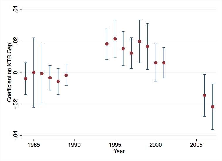
Figure 1: Dynamics
Notes: This figure is constructed in two steps: First, we run a regression of industry level returns on the set of controls in the
baseline regression, as well as industry fixed-effects and month-fixed effects. The second stage takes the residuals from the first
stage, and regresses them on the NTR gap in 5-year rolling windows. For example, the datapoint for 1994 uses data from 1990
to 1994. The blue lines surrounding the point estimates (red dots) are 95% confidence intervals, calculated based on standard
errors clustered at the industry-level.
The graph shows that the positive association between the NTR gap and stock returns
was significant throughout the entire 1990-2001 period, but it was stronger in the first years
of the decade (although the coefficient are not statistically different from each other). This is
consistent with the fact that there was greater uncertainty about the legislation passage in
the years 1990-1992, as suggested by the fact that in those years the House voted in favor of
revoking NTR status to China.
In contrast, in the 1980-1989 control period the relationship between NTR gap and stock
returns was not significantly different from zero, while after 2001 the coefficient is negative
and significant. This negative relationship in the post period can likely be explained with a
negative effect of PNTR on high-gap firms cash-flows, as documented by Greenland et al.
10(2019). This may also explain the larger DID coefficient that we find in Table 1 when we
use the 2002-2007 control period. We discuss in detail in Section 4 how the cash-flow effect
could affect our results. However, it is important to note that the negative relative returns
observed in the post period do not alter the main conclusions of the paper, since the portfolio
analysis we undertake in Section 3 documents a TPU risk factor only in the uncertainty
period 1990-2001.
2.4 Robustness
In Table A.3 in Appendix 6.1 we perform several exercises to gauge the robustness of our
baseline results. First, we control for the possibility that high-gap and low-gap industries may
load differently on risk factors known to predict returns. To this end, we first run regressions
using daily data in 5-year rolling windows to estimate the betas of each industry portfolio on
the Fama and French (2015) factors. We then interact the estimated betas, lagged by one
month, with the uncertainty dummy, and add them to the baseline regression. Column (1)
shows that the DID coefficient is very close to the baseline. Column (2) reports the results of
the baseline specification, but with standard errors clustered at both industry and month
level, as in Petersen (2009), to account for the potential autocorrelation of the residuals.
With double clustering, the coefficient of interest is still significant at the 5% level.10 Column
(3) weighs observations by the industry’s previous year market capitalization, as in standard
portfolio analysis; column (4) uses an equally weighted regression; column (5) includes an
interaction between all control variables and the treatment period dummy, to ensure that the
other covariates do not generate differential average returns during the uncertainty period
(see e.g. Gagliardini et al. (2016)). We can see that in all these specifications the DID
coefficient is very similar to the baseline. In addition, column (4) suggests that weighting
the observations leads to a more precise point estimate, which is smaller but not statistically
different from the baseline.
One concern with our identification strategy is that the US government could have set
high NTR tariff rates to protect industries that they expected to perform poorly. In this
case, while the non-NTR rates are exogenous because they were set by the Smoot-Hawley
act, NTR rates are not. A second related concern is that the decision to vote on legislation to
revoke China’s temporary NTR status could have motivated by economic reasons, rather than
geo-political reasons, i.e. the Tiananmen Square Massacre. This could generate an omitted
variable problem in our regressions, leading to biased estimates. To mitigate these concerns,
10
We do not weight observations when we double cluster the standard errors, because that leads to a not
well-defined covariance matrix. This could be the result of a particular correlation structure within clusters.
11we follow Pierce and Schott (2016) and estimate a two-stage least squares specification in
which we instrument the baseline DID term, U ncertaintyt × Gapi,y−1 , with an interaction of
the uncertainty indicator and the Smoot-Hawley non-NTR rates, U ncertaintyt × N N T Ri . As
reported in column (6) of Table 3, the DID coefficient is positive, statistically significant and
close to the baseline. Finally, column (6) reports the results when holding the NTR gap at
its level in 1990, the year the uncertainty started, with similar results.11
3 A Risk Premium for Tariff Uncertainty
Our empirical results show that high gap industries had higher average returns, relative to
low gap industries, between 1990 and 2001. In this section, we argue that this difference in
returns was a risk premium for exposure to tariff uncertainty. We first perform a portfolio
analysis which shows that, only in the uncertainty period 1990-2001, a portfolio long high-gap
sectors and short low gap industries had positive and significant returns. We then present
additional empirical evidence on discount rate effects and realized volatility that support our
risk premium hypothesis.
3.1 Conceptual framework
In any asset pricing model (see e.g. Cochrane (2009) and Duffie (2010)), the maximization
problem of the representative investor implies the following relationship:
E (rit − rf ) ∝ −Cov (SDFt , rit ) (3)
Equation (3) states that the expected excess return of any asset i is inversely proportional to
the covariance of the asset’s return with the Stochastic Discount Factor (SDF). Intuitively,
stocks that covary negatively with the SDF are riskier because they pay less in bad states
of the world, and thus require higher expected returns as compensation for risk-averse
investors.12 Empirically, expected returns are estimated using average returns, computed
over long periods of time.
To fully characterize the SDF, further assumptions about the economy are needed. The key
elements in defining the SDF are the factors that affect the marginal utility of consumption.
11
Additional results not reported for brevity show that our findings are robust if i) we use the industry
classification in CRSP, and ii) we exclude the computer and electronics industries that experienced the
dot-com crash in 2000-2001, iii) we extend the sample to 2017.
12
For example, with CRRA utility and time-separable preferences, the SDF is proportional to the marginal
utility of consumption. See also footnote 16.
12Given our setting, we think it is appropriate to start with the well-known frameworks in
Pastor and Veronesi (2012) and Pástor and Veronesi (2013). In these models, stock dividends
depend on the government policy, which is uncertain, and thus any policy change affects the
future marginal utility. This implies that government policy enters the SDF, i.e. investors
require an additional compensation for exposure to policy uncertainty. In the context of
our analysis, this means that stocks more exposed to TPU, i.e. stocks with higher NTR
gap, should have a higher (in absolute value) covariance with the component of the SDF
associated with TPU. From equation (3), this implies higher expected returns.13
In the next section, we follow the vast literature on empirical asset pricing (see e.g. Nagel
(2013) and Fama and French (2015)) and test this hypothesis by ranking stocks according to
their exposure to TPU and forming value-weighted portfolios. We then present additional
empirical evidence, consistent with the predictions of the Pastor and Veronesi (2012) model,
that supports our risk premium hypothesis.
3.2 Portfolio analysis
In order to estimate the risk premium associated with exposure to TPU, we rank the industries
in our sample in 3 sub-groups, based on their NTR gap in 1990, the year the uncertainty began.
The groups are above/below/between the 33rd and 66th percentiles. We then construct
value-weighted portfolios, with weights proportional to each firm’s market capitalization
in the previous month, and calculate monthly returns between 1990 and 2001. We then
construct a ‘‘Trade Policy Uncertainty’’ (TPU) portfolio, which is the difference in returns
between the portfolios containing firms with the highest and lowest gaps, divided by two.
We then run the following regression, separately for each portfolio p:14
rtp = αp + F ′t β + ǫt (4)
where rtp is the excess return on portfolio p in month t, and F t is a vector containing the
5 Fama and French (2015) factors: the market portfolio minus the risk-free rate, the size
13
This conclusion implicitly assumes that: i) the covariance between the component of the SDF associated
with jumps in TPU and stock returns is negative, i.e. increases in TPU are perceived as bad states of the
world by investors, and ii) the loading on the TPU factor in the SDF is positive. Both endogenously hold
in Pastor and Veronesi (2012) (see Proposition 6), and are consistent with a vast literature arguing that
increases in uncertainty are detrimental for the economy (see e.g. Bloom et al. (2007), Bloom (2009) and
Bachmann et al. (2013)).
14
The implicit assumption is that the loadings on other risk-factors, such as the Fama and French (2015)
factors, are randomly distributed across high and low gap firms. In addition, under standard assumptions on
the stochastic process for the returns, one can show that the SDF is linear in its arguments (see e.g. Pastor
and Veronesi (2012)). This implies that by constructing a portfolio that goes long high-gap firms, and short
low-gap firms, we can effectively isolate exposure to TPU.
13factor (small minus big), the value factor (high minus low), the profitability factor (robust
minus weak), and the investment factor (conservative minus aggressive).15 Our hypothesis is
that industries more exposed to policy uncertainty should command higher expected returns,
because investors require compensation for such exposure, as in Pastor and Veronesi (2012).
If our hypothesis is correct, then the estimated constant αp in equation (4) should be: i)
monotonically increasing as we go from low to high gap portfolios, and ii) positive and
significant for the TPU portfolio.
Our results in Table 2 show that the TPU portfolio had an αp of 0.005 per month during
the uncertainty period, significant at the 1% level. Furthermore, the constant is monotonically
increasing as we go from the low gap to high gap portfolios. The estimated coefficient implies
that the TPU portfolio, long high-gap firms and short low-gap firms, would have earned
6% per year throughout the 1990-2001 period. Therefore, trade policy uncertainty was a
systematic factor that could not be diversified away across stocks with similar NTR gaps.16
15
We obtain the monthly returns on these factors from Ken French’s website: https://mba.tuck.
dartmouth.edu/pages/faculty/ken.french/data_library.html.
16
Additional evidence in favor of the risk premium hypothesis comes from the consumption-based
capital
−γ
Ct+1
asset pricing model. Under power utility, the risk premium is simply proportional to −Cov β Ct , rit ,
where γ is the relative risk aversion of the representative consumer, rit is the return of asset i, and CCt+1
t
is
the growth rate of aggregate consumption. We estimate this correlation with a range of relative risk aversion
from 1 to 30, gross growth of US private consumption expenditure from the FRED database, the S&P500
market portfolio, and the TPU portfolio constructed as described above. We find that the correlation between
the stochastic discount factor and the TPU portfolio payoff is between -0.20 and -0.22, and statistically
significant between 1990 and 2001. Instead, in the 1980-1989 and 2001-2007 periods such correlation is not
statistically significant.
14Table 2: Portfolio analysis
Dep. variable: Monthly returns, Rtp
Low Gap Medium Gap High Gap TPU
Market 0.849*** 1.098*** 0.983*** 0.067
(0.05) (0.06) (0.08) (0.05)
Size -0.131** 0.220*** 0.133 0.132**
(0.05) (0.08) (0.08) (0.06)
Value -0.237** -0.031 -0.294** -0.029
(0.09) (0.11) (0.12) (0.09)
Profitability 0.243*** -0.076 -0.240** -0.241***
(0.07) (0.08) (0.11) (0.08)
Investment 0.742*** -0.310* -0.601*** -0.671***
(0.15) (0.17) (0.16) (0.13)
αp -0.002 -0.001 0.008*** 0.005***
(0.00) (0.00) (0.00) (0.00)
Realized Volatility 0.034 0.061 0.072 0.032
R2 0.713 0.881 0.878 0.694
Observations 144 144 144 144
Sample Period 1990-2001 1990-2001 1990-2001 1990-2001
Notes: This table contains selected estimates from the following regression, using data from 1990-2001:
rtp = F ′t β + αp + ǫt
where rtp is the return on portfolio p in month t. F ′t is a vector containing the 5 Fama-French factors: Market, Size, Value,
Profitability and Investment. Robust standard errors are in parenthesis. *** p < 0.01, ** p < 0.05, * p < 0.10
Table 2 also reports the realized volatility of each portfolio computed during the same
period. We can see that the realized volatility increases monotonically as we go from the low
gap to the high gap portfolio. This is also consistent with the Pastor and Veronesi (2012)
model, which predicts a positive relationship between exposure to uncertainty and volatility.
Table 3 repeats the same portfolio analysis but using the 1980-1989 and 2001-2007 periods.
The table documents that during the control periods, high-gap industries did not have
economically large or statistically significant alphas, suggesting that the risk premium was
earned only during the uncertainty period, consistent with our hypothesis.
15Table 3: Portfolio analysis, control periods
Dep. variable: Monthly returns, Rtp
TPU TPU
Market -0.014 0.074
(0.04) (0.07)
Size 0.229*** 0.114*
(0.07) (0.06)
Value -0.343*** -0.294**
(0.10) (0.12)
Profitability -0.296*** -0.323**
(0.10) (0.14)
Investment -0.02 0.093
(0.13) (0.14)
αp 0.002 0
(0.00) 0.00
Realized Volatility 0.018 0.019
R2 0.419 0.544
Observations 120 72
Sample Period 1980-1989 2002-2007
Notes: This table contains selected estimates from the following regression:
rtp = F ′t β + αp + ǫt
where rtp is the return on portfolio p in month t. F ′t is a vector containing the 5 Fama-French factors: Market, Size, Value,
Profitability and Investment. Robust standard errors are in parenthesis. *** p < 0.01, ** p < 0.05, * p < 0.10
3.2.1 The determinants of the risk premium
We now investigate which economic forces interact with exposure to TPU and determine
the expected returns. We first examine how the level of trade protection interacts with the
exposure to trade policy uncertainty. Specifically, we form portfolios by double-sorting the
industries according to both the NTR gap in 1990 and the NTR tariff rate in 1990. To do
this, we calculate the median of the NTR gap in 1990, and the median of the NTR rate
in 1990. We then do a 2 by 2 sort to form 4 total portfolios. Table 4 shows that the risk
premium was earned mostly by industries with a low level of NTR rate, i.e. industries less
protected by trade policy from foreign competition. This suggests that a lack of protection
from import competition can amplify the risk premium for TPU.
16Table 4: TPU and NTR rates
Dep. variable: Monthly returns, Rtp
TPU-Low TPU-High
Market 0.028 0.085
(0.07) (0.08)
Size 0.078 0.1
(0.08) (0.09)
Value -0.057 0.137
(0.12) (0.13)
Profitability -0.278*** -0.18
(0.10) (0.11)
Investment -0.683*** -0.264
(0.17) (0.22)
αp 0.007*** -0.001
(0.00) (0.00)
R2 0.552 0.203
Observations 144 144
Sample Period 1990-2001 1990-2001
Notes: This table contains selected estimates from the following regression, using data from 1990-2001:
rtp = F ′t β + αp + ǫt
where rtp is the return on portfolio p in month t. F ′t is a vector containing the 5 Fama-French factors: Market, Size, Value,
Profitability and Investment. Robust standard errors are in parenthesis. *** p < 0.01, ** p < 0.05, * p < 0.10
Motivated by this result, we examine the relationship between our TPU factor and the
globalization risk premium, estimated in Barrot et al. (2018) with data on industry-level
shipping costs. We first simply add their factor as control in addition to the baseline 5 factors.
Table 5 shows that the high-gap portfolio loads positively on the globalization factor, but the
alpha remains highly significant and very close to the baseline, suggesting that the TPU risk
premium is not explained by exposure to globalization.
17Table 5: TPU and Globalization Risk Factor
Low Gap Medium Gap High Gap TPU
Market 0.841*** 1.093*** 0.947*** 0.053
(0.05) (0.07) (0.07) (0.05)
Size -0.123** 0.225*** 0.169** 0.146**
(0.06) (0.08) (0.08) (0.06)
Value -0.193* -0.001 -0.093 0.05
(0.10) (0.12) (0.11) (0.09)
Profitability 0.262*** -0.063 -0.153 -0.207***
(0.07) (0.08) (0.10) (0.08)
Investment 0.753*** -0.303* -0.552*** -0.653***
(0.15) (0.17) (0.15) (0.13)
Globalization 0.057 0.037 0.256*** 0.100**
(0.05) (0.07) (0.05) (0.05)
αp -0.002 -0.001 0.005** 0.004**
(0.00) (0.00) (0.00) (0.00)
R2 0.718 0.881 0.898 0.710
Observations 144 144 144 144
Sample Period 1990-2001 1990-2001 1990-2001 1990-2001
Notes: This table contains selected estimates from the following regression, using data from 1990-2001:
rtp = F ′t β + αp + ǫt
where rtp is the return on portfolio p in month t. F ′t is a vector containing the 5 Fama-French factors: Market, Size, Value,
Profitability and Investment, plus the Globalization Factor estimated in Barrot et al (2018). Robust standard errors are in
parenthesis. *** p < 0.01, ** p < 0.05, * p < 0.10
In addition, we double sort portfolios on the NTR gap in 1990 and on the shipping costs
from Barrot et al. (2018). Table 6 reports that, within high-gap industries, the TPU risk
premium was earned by industries with lower shipping costs, i.e. sectors that were exposed
more to globalization. This suggests another amplifying factor of the risk premium for trade
policy uncertainty.
18Table 6: TPU and Shipping costs
Dep. variable: Monthly returns, Rtp
TPU-Low TPU-High
Market 0.003 0.123**
(0.09) (0.05)
Size 0.115 0.126**
(0.10) (0.05)
Value 0.432** -0.393***
(0.17) (0.08)
Profitability -0.441*** 0.038
(0.12) (0.07)
Investment -1.087*** 0.214*
(0.21) (0.12)
αp 0.006** 0.001
(0.00) (0.00)
R2 0.453 0.462
Observations 144 144
Sample Period 1990-2001 1990-2001
Notes: This table contains selected estimates from the following regression, using data from 1990-2001:
rtp = F ′t β + αp + ǫt
where rtp is the return on portfolio p in month t. F ′t is a vector containing the 5 Fama-French factors: Market, Size, Value,
Profitability and Investment. Robust standard errors are in parenthesis. *** p < 0.01, ** p < 0.05, * p < 0.10
Lastly, we study another channel through which TPU may have affected the riskiness
of US firms. Table 7 documents that, within high-gap industries, industries with a higher
share of inputs expenditures from China throughout the 1990-2001 period earned a larger
risk premium.17 This suggests that uncertainty about the cost of production, deriving from
uncertainty on the tariffs imposed on intermediate inputs from China, is a risk factor that
was also priced by financial markets.
17
We use data from WIOD to compute the share of expenditures of each downstream US industry on each
upstream industry from China. Since the sectors in the WIOD are more aggregated than the industries in
our sample, we assume that this share is constant across industries within each WIOD sector.
19Table 7: TPU and inputs from China
Dep. variable: Monthly returns, Rtp
TPU-Low TPU-High
Market 0.037 0.043
(0.07) (0.07)
Size 0.116 0.124*
(0.09) (0.07)
Value 0.047 0.047
(0.10) (0.12)
Profitability -0.095 -0.260***
(0.08) (0.09)
Investment -0.146 -0.770***
(0.15) (0.16)
αp 0.002 0.005***
(0.00) (0.00)
R2 0.117 0.620
Observations 144 144
Sample Period 1990-2001 1990-2001
Notes: This table contains selected estimates from the following regression, using data from 1990-2001:
rtp = F ′t β + αp + ǫt
where rtp is the return on portfolio p in month t. F ′t is a vector containing the 5 Fama-French factors: Market, Size, Value,
Profitability and Investment. Robust standard errors are in parenthesis. *** p < 0.01, ** p < 0.05, * p < 0.10
3.3 Discount rate effect
In Section 3.1, we argue that high-gap firms had higher average returns than low-gap firms
between 1990 and 2001 because investors required a risk premium for exposure to trade policy
uncertainty. In any asset pricing model, the stock price of firm i in period t equals:
Di,t+1
Pi,t = , (5)
ri − g i
where Di,t+1 is the cash-flow at t + 1, ri is a weighted-average of all future discount rates,
and gi is a weighted-average of all future growth rates (see e.g. Campbell and Shiller (1988)).
The discount rate embeds firm i’s loadings on all priced risk factors which, as argued in
Section 3.1, should include trade policy uncertainty. Equation (5) implies that if there is
a sudden jump in TPU, the discount rate increases and the stock price decreases. Thus, if
we could identify the date when the uncertainty on China’s NTR status began, we should
observe a sudden decrease in stock prices for exposed industries. As shown in Pastor and
20Veronesi (2012), this discount rate effect at the announcement of a new policy should be
stronger for industries more exposed to TPU, i.e. the ones with higher NTR gap.
We look at the stock price responses around the days in which the uncertainty about
China’s tariff status reasonably began. In particular, while the Tiananmen Square Massacre
happened on June 4, 1989, the first resolution to revoke China’s NTR status was introduced
in the House on May 24, 1990, by Rep. Donald Pease (H.R. 4939), and it was reported by
the Committee on Ways and Means on July 23, 1990 (H. Rept. 101-620).18 As introduced,
the bill would have directed the President to take new conditions – involving substantial
progress on human rights violations – into account when extending China’s MFN status
beginning in 1991 (see Dumbaugh (1998)).19
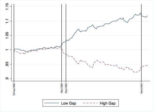
We examine value-weighted portfolios of high-gap and low-gap firms, defined as having
NTR gaps above/below the median in 1990. We work with market-adjusted returns of these
portfolios to take out a common mean component over the period of interest. Figure 2
documents the value of $1 invested in each of these portfolios on May 24, 1990. We can
see that, from when the bill was introduced until July, 1990, high and low gap firms were
following the same trend. On July 18, 1990 the bill was ordered to be reported by the
Committee on Ways and Means, and it was actually reported by the Committee on July 23,
1990 (H. Rept. 101-620). Since then, i.e. when it became known to the public that the House
was considering revoking China’s NTR status, high-gap firms’ market-adjusted stock returns
started to decrease relative to low-gap firms. This suggests a strong discount rate effect
pushing down prices for tradeable sectors more exposed to the newly introduced trade policy
uncertainty. Interestingly, when the bill was actually approved by the House on October
18, 1990, there was no significant impact on stock prices, suggesting that the markets had
already priced in the increased TPU.
18
The Tiananmen Square Massacre happened 3 days after President Bush’s MFN extension recommen-
dation for 1989, and no resolution was introduced in the Congress in 1989 to disapprove the President’s
recommendation. The U.S. response to Tiananmen Square that year consisted of two sets of non-MFN-related
sanctions announced by President Bush (on June 5 and June 20, 1989), and a series of bills that Congress
considered which were designed to codify the President’s actions and expand their scope. See Dumbaugh
(1998).
19
See https://www.congress.gov/bill/101st-congress/house-bill/4939.
21Figure 2: Effect of Introducing Uncertainty
Notes: The figure plots the value of 1 dollar invested in value-weighted portfolios of high and low gap industries on 5/24/1990.
Another explanation for the drop in stock prices for high NTR gap firms could have been
a decrease in gi .20 This may have occurred, for example, if investors believed that increased
policy uncertainty would have led high-gap firms to hold cash, instead of paying dividends or
buying back shares, relatively more than low-gap firms. If investors had perfect foresight,
the effect of increased uncertainty on all future expected dividend growth rates should have
been reflected in prices. To test this hypothesis, we calculate realized dividend growth rates
for the 3 portfolios formed in Section 3.2. We find that between 1990 and 2001, the dividend
growth rate of high-gap firms was not statistically significantly different from the one of
low-gap firms. This suggests that, even in the perfect foresight case, a change in gi was likely
not responsible for the price drop in Figure 2.
20
Of course, another reason for the drop in stock price could have been a relative decrease in the next
period’s dividends, Di,t+1 . However, the literature has shown that uncertainty typically has long-run effects
that would not show up instantaneously on dividends (see e.g. Bloom (2009) and Barrero et al. (2017)). In
fact, when we look at dividends paid in 1991, they actually increased relatively more for high-gap firms.
223.4 Realized Volatility
We investigate whether uncertainty about China’s trade status was also associated with
more volatile stock prices around days where policy-related news was released. Intuitively,
regardless of whether the policy change is perceived as good or bad by investors, firms more
exposed to such policy changes should have larger responses (in absolute terms) than less
exposed firms, as argued both theoretically and empirically in Pastor and Veronesi (2012),
Boutchkova et al. (2012) and Baker et al. (2019).
We test this hypothesis with the following regression:
RVit = α + θ1 · N T RGapi,1990 + θ2 · Dt + θ3 · Dt · N T RGapi,1990 + ǫit (6)
where RVit is the realized volatility of firm i in day t, computed as the sum of the squared
daily returns, Dt is a dummy equal to 1 if t is between 3 days before and 3 after a policy
event, and N T RGapi,1990 is the NTR gap in 1990 of the firm’s industry. We estimate this
regression at the firm-day level so we can i) account for unconditional differences in volatility
among high and low gap firms between 1990 and 2001, and ii) cluster the standard errors at
the firm level. We do not control for differences in firm fundamentals as, given that we are
only including a tight window around the announcement, we expect the announcement to be
the main factor driving differences in volatility.
We focus on three key policy announcements: i) 10/10/2000, when China was granted
permanent NTR, conditional on joining the WTO; ii) 12/11/2001, when China joined the
WTO; iii) 1/2/2002, the day the PNTR actually went into effect. We also include all days in
which the US Congress voted to revoke the NTR status to China, from 1990 to 2001.
Table 8 documents that, during the tariff uncertainty period, i) firms in high-gap industries
had significantly higher average realized volatility than firms in low-gap industries, and ii) this
difference was larger around relevant policy days. To ensure that the higher unconditional
volatility of high-gap firms does not drive the result on the event dates, we select random
placebo announcement days each year. The interaction term on these placebo days is not
significant, confirming that the increased volatility of high-gap firms is specific to key policy
days.
23Table 8: Realized Volatility around Policy Days
Dep. variable: Realized Volatility, RVit
Actual days Placebo days
Day -0.0189 0.0645***
(0.00) (0.00)
Gapi,1990 2.17*** 2.16***
(0.00) (0.00)
Gapi,1990 × Day 0.547*** -0.22
(0.00) (0.00)
Constant 0.309*** 0.307***
(0.00) (0.00)
R2 0.004 0.004
Observations 8,730,368 8,288,900
Notes: This table contains selected estimates from versions of the following regression, run at the industry(i)/month(t) level
using data from 1980-2007:
RVit = α + θ1 · N T RGapi,1990 + θ2 · Dt + θ3 · Dt · N T RGapi,1990 + ǫit
where RVit is the sum of squared daily returns for firm i from t − 3 to t + 3 where t is the event-date of interest. Robust
standard errors, clustered at the firm level, are in parenthesis. *** p < 0.01, ** p < 0.05, * p < 0.10
4 Alternative Explanations
In this section we discuss a number of alternative explanations that could potentially ratio-
nalize our results, and show that they are not consistent with the empirical evidence. This
additional set of results provides strong evidence in favor of our explanation that exposure to
TPU is a source of risk that is priced in the cross-section of stock returns.
4.1 Expected Cash-flow Effect
A potential explanation for our results could be that the higher returns for high-gap industries
in the uncertainty period were driven by the response of stock prices to news and policy-related
events, rather than by a change in the risk premium. If capital markets are efficient, stock
prices adjust quickly after a news announcement, incorporating any changes in expected
future cash-flows, as recently shown by Breinlich (2014) and Greenland et al. (2019).
In order to disentangle the effect of expected cash flows on stock returns, we repeat our
portfolio analysis but exclude a window of 3 days before and after each policy-related event.
We use the same days as in the previous section: all the Congressional voting days, and three
key policy announcements days. We sum daily log-returns to compute monthly returns.
24You can also read