DECOUPLING EXPLORATION AND EXPLOITATION FOR META-REINFORCEMENT LEARNING WITHOUT SACRI-FICES
←
→
Page content transcription
If your browser does not render page correctly, please read the page content below
Under review as a conference paper at ICLR 2021

D ECOUPLING E XPLORATION AND E XPLOITATION FOR
M ETA -R EINFORCEMENT L EARNING WITHOUT S ACRI -
FICES

 Anonymous authors
 Paper under double-blind review

                                              A BSTRACT
           The goal of meta-reinforcement learning (meta-RL) is to build agents that can
           quickly learn new tasks by leveraging prior experience on related tasks. Learning
           a new task often requires both exploring to gather task-relevant information and
           exploiting this information to solve the task. In principle, optimal exploration and
           exploitation can be learned end-to-end by simply maximizing task performance.
           However, such meta-RL approaches struggle with local optima due to a chicken-
           and-egg problem: learning to explore requires good exploitation to gauge the
           exploration’s utility, but learning to exploit requires information gathered via
           exploration. Optimizing separate objectives for exploration and exploitation can
           avoid this problem, but prior meta-RL exploration objectives yield suboptimal
           policies that gather information irrelevant to the task. We alleviate both concerns
           by constructing an exploitation objective that automatically identifies task-relevant
           information and an exploration objective to recover only this information. This
           avoids local optima in end-to-end training, without sacrificing optimal exploration.
           Empirically, D REAM substantially outperforms existing approaches on complex
           meta-RL problems, such as sparse-reward 3D visual navigation.1

1       I NTRODUCTION
A general-purpose agent should be able to perform multiple related tasks across multiple related
environments. Our goal is to develop agents that can perform a variety of tasks in novel environments,
based on previous experience and only a small amount of experience in the new environment. For
example, we may want a robot to cook a meal (a new task) in a new kitchen (the environment)
after it has learned to cook other meals in other kitchens. To adapt to a new kitchen, the robot must
both explore to find the ingredients, and use this information to cook. Existing meta-reinforcement
learning (meta-RL) methods can adapt to new tasks and environments, but, as we identify in this
work, struggle when adaptation requires complex exploration.
In the meta-RL setting, the agent is presented with a set of meta-training problems, each in an
environment (e.g., a kitchen) with some task (e.g., make pizza); at meta-test time, the agent is given a
new, but related environment and task. It is allowed to gather information in a few initial (exploration)
episodes, and its goal is to then maximize returns on all subsequent (exploitation) episodes, using this
information. A common meta-RL approach is to learn to explore and exploit end-to-end by training
a policy and updating exploration behavior based on how well the policy later exploits using the
information discovered from exploration (Duan et al., 2016; Wang et al., 2016a; Stadie et al., 2018;
Zintgraf et al., 2019; Humplik et al., 2019). With enough model capacity, such approaches can express
optimal exploration and exploitation, but they create a chicken-and-egg problem that leads to bad
local optima and poor sample efficiency: Learning to explore requires good exploitation to gauge the
exploration’s utility, but learning to exploit requires information gathered via exploration; therefore,
with only final performance as signal, one cannot be learned without already having learned the other.
For example, a robot chef is only incentivized to explore and find the ingredients if it already knows
how to cook, but the robot can only learn to cook if it can already find the ingredients by exploration.
To avoid the chicken-and-egg problem, we propose to optimize separate objectives for exploration and
exploitation by leveraging the problem ID—an easy-to-provide unique one-hot for each training meta-
    1
        Project web page: https://anonymouspapersubmission.github.io/dream/

                                                    1
Under review as a conference paper at ICLR 2021

training task and environment. Some prior works (Humplik et al., 2019; Kamienny et al., 2020) also
use these problem IDs, but not in a way that avoids the chicken-and-egg problem. Others (Rakelly
et al., 2019; Zhou et al., 2019b; Gupta et al., 2018; Gurumurthy et al., 2019; Zhang et al., 2020)
also optimize separate objectives, but their exploration objectives learn suboptimal policies that
gather task-irrelevant information (e.g., the color of the walls). Instead, we propose an exploitation
objective that automatically identifies task-relevant information, and an exploration objective to
recover only this information. We learn an exploitation policy without the need for exploration, by
conditioning on a learned representation of the problem ID, which provides task-relevant information
(e.g., by memorizing the locations of the ingredients for each ID / kitchen). We also apply an
information bottleneck to this representation to encourage discarding of any information not required
by the exploitation policy (i.e., task-irrelevant information). Then, we learn an exploration policy
to only discover task-relevant information by training it to produce trajectories containing the same
information as the learned ID representation (Section 4). Crucially, unlike prior work, we prove that
our separate objectives are consistent: optimizing them yields optimal exploration and exploitation,
assuming expressive-enough policy classes and enough meta-training data (Section 5.1).
Overall, we present two core contributions: (i) we articulate and formalize a chicken-and-egg coupling
problem between optimizing exploration and exploitation in meta-RL (Section 4.1); and (ii) we
overcome this with a consistent decoupled approach, called D REAM: Decoupling exploRation and
ExploitAtion in Meta-RL (Section 4.2). Theoretically, in a simple tabular example, we show that
addressing the coupling problem with D REAM provably improves sample complexity over existing
end-to-end approaches by a factor exponential in the horizon (Section 5). Empirically, we stress test
D REAM’s ability to learn sophisticated exploration strategies on 3 challenging, didactic benchmarks
and a sparse-reward 3D visual navigation benchmark. On these, D REAM learns to optimally explore
and exploit, achieving 80% higher returns than existing state-of-the-art approaches (P EARL, E-RL2 ,
I MPORT, VARI BAD), which struggle to learn an effective exploration strategy (Section 6).

2    R ELATED W ORK
We draw on a long line of work on learning to adapt to related tasks (Schmidhuber, 1987; Thrun &
Pratt, 2012; Naik & Mammone, 1992; Bengio et al., 1991; 1992; Hochreiter et al., 2001; Andrychow-
icz et al., 2016; Santoro et al., 2016). Many meta-RL works focus on adapting efficiently to a new
task from few samples without optimizing the sample collection process, via updating the policy
parameters (Finn et al., 2017; Agarwal et al., 2019; Yang et al., 2019; Houthooft et al., 2018; Men-
donca et al., 2019), learning a model (Nagabandi et al., 2018; Sæmundsson et al., 2018; Hiraoka et al.,
2020), multi-task learning (Fakoor et al., 2019), or leveraging demonstrations (Zhou et al., 2019a). In
contrast, we focus on problems where targeted exploration is critical for few-shot adaptation.
Approaches that specifically explore to obtain the most informative samples fall into two main
categories: end-to-end and decoupled approaches. End-to-end approaches optimize exploration and
exploitation end-to-end by updating exploration behavior from returns achieved by exploitation (Duan
et al., 2016; Wang et al., 2016a; Mishra et al., 2017; Rothfuss et al., 2018; Stadie et al., 2018; Zintgraf
et al., 2019; Humplik et al., 2019; Kamienny et al., 2020; Dorfman & Tamar, 2020). These approaches
can represent the optimal policy (Kaelbling et al., 1998), but they struggle to escape local optima
due to a chicken-and-egg problem between learning to explore and learning to exploit (Section 4.1).
Several of these approaches (Humplik et al., 2019; Kamienny et al., 2020) also leverage the problem
ID during meta-training, but they still learn end-to-end, so the chicken-and-egg problem remains.
Decoupled approaches instead optimize separate exploration and exploitation objectives, via, e.g.,
Thompson-sampling (TS) (Thompson, 1933; Rakelly et al., 2019), obtaining exploration trajectories
predictive of dynamics or rewards (Zhou et al., 2019b; Gurumurthy et al., 2019; Zhang et al., 2020),
or exploration noise (Gupta et al., 2018). While these works do not identify the chicken-and-egg
problem, decoupled approaches coincidentally avoid it. However, existing decoupled approaches,
including ones (Rakelly et al., 2019) that leverage the problem ID, do not learn optimal exploration:
TS (Rakelly et al., 2019) explores by guessing the task and executing a policy for that task, and
hence cannot represent exploration behaviors that are different from exploitation (Russo et al., 2017).
Predicting the dynamics (Zhou et al., 2019b; Gurumurthy et al., 2019; Zhang et al., 2020) is inefficient
when only a small subset of the dynamics are relevant to solving the task. In contrast, we propose
a separate mutual information objective for exploration, which both avoids the chicken-and-egg
problem and yields optimal exploration when optimized (Section 5). Past work (Gregor et al., 2016;

                                                    2
Under review as a conference paper at ICLR 2021

                     r0        r1                 r0        r1                  r0        r1                            r0        r1
                s0        s1   ...   sT      s0        s1        ... ...   s0        s1        ...                s0         s1   ...   sT
    Cook soup   exploration episode       exploitation episode 1     exploitation episode N          Cook pizza   exploration episode        ...   ...
                (gather information)            (solve the task and maximize returns)                             (gather information)
                                          Trial 1                                                                      Trial 2

Figure 1: Meta-RL setting: Given a new environment and task, the agent is allowed to first explore and gather
information, and then must use this information to solve the task in subsequent exploitation episodes.
Houthooft et al., 2016; Eysenbach et al., 2018; Warde-Farley et al., 2018) also optimize mutual
information objectives, but not for meta-RL.

3      P RELIMINARIES
Meta-reinforcement learning. The meta-RL setting considers a family of Markov decision processes
(MDPs) hS, A, Rµ , Tµ i with states S, actions A, rewards Rµ , and dynamics Tµ , indexed by a one-
hot problem ID µ ∈ M, drawn from a distribution p(µ). Colloquially, we refer to the dynamics as the
environment, the rewards as the task, and the entire MDP as the problem. Borrowing terminology from
Duan et al. (2016), meta-training and meta-testing both consist of repeatedly running trials. Each
trial consists of sampling a problem ID µ ∼ p(µ) and running N + 1 episodes on the corresponding
problem. Following prior evaluation settings (Finn et al., 2017; Rakelly et al., 2019; Rothfuss et al.,
2018; Fakoor et al., 2019), we designate the first episode in a trial as an exploration episode consisting
of T steps for gathering information, and define the goal as maximizing the returns in the subsequent
N exploitation episodes (Figure 1). Following Rakelly et al. (2019); Humplik et al. (2019); Kamienny
et al. (2020), the easy-to-provide problem ID is available for meta-training, but not meta-testing trials.
We formally express the goal in terms of an exploration policy π exp used in the exploration episode
and an exploitation policy π task used in exploitation episodes, but these policies may be the same
or share parameters. Rolling out π exp in the exploration episode produces an exploration trajectory
τ exp = (s0 , a0 , r0 , . . . , sT ), which contains information discovered via exploration. The exploitation
policy π task may then condition on τ exp and optionally, its history across all exploitation episodes in a
trial, to maximize exploitation episode returns. The goal is therefore to maximize:
                                 J (π exp , π task ) = Eµ∼p(µ),τ exp ∼πexp V task (τ exp ; µ) ,

                                                                                                          (1)
where V task (τ exp ; µ) is the expected returns of π task conditioned on τ exp , summed over the N exploita-
tion episodes in a trial with problem ID µ.
End-to-end meta-RL. A common meta-RL approach (Wang et al., 2016a; Duan et al., 2016; Rothfuss
et al., 2018; Zintgraf et al., 2019; Kamienny et al., 2020; Humplik et al., 2019) is to learn to explore
and exploit end-to-end by directly optimizing J in (1), updating both from rewards achieved during
exploitation. These approaches typically learn a single recurrent policy π(at | st , τ:t ) for both
exploration and exploitation (i.e., π task = π exp = π), which takes action at given state st and history
of experiences spanning all episodes in a trial τ:t = (s0 , a0 , r0 , . . . , st−1 , at−1 , rt−1 ). Intuitively, this
policy is learned by rolling out a trial, producing an exploration trajectory τ exp and, conditioned on
τ exp and the exploitation experiences so far, yielding some exploitation episode returns. Then, credit
is assigned to both exploration (producing τ exp ) and exploitation by backpropagating the exploitation
returns through the recurrent policy. Directly optimizing the objective J this way can learn optimal
exploration and exploitation strategies, but optimization is challenging, which we show in Section 4.1.

4      D ECOUPLING E XPLORATION AND E XPLOITATION
4.1      T HE P ROBLEM WITH C OUPLING E XPLORATION AND E XPLOITATION
We begin by showing that end-to-end optimization struggle with local optima due to a chicken-and-
egg problem. Figure 2a illustrates this. Learning π exp relies on gradients passed through π task . If π task
cannot effectively solve the task, then these gradients will be uninformative. However, to learn to
solve the task, π task needs good exploration data (trajectories τ exp ) from a good exploration policy
π exp . This results in bad local optima as follows: if our current (suboptimal) π task obtains low rewards
                                         exp
with a good informative trajectory τgood     , the low reward would cause π exp to learn to not generate
  exp                   exp                                   exp
τgood . This causes π to instead generate trajectories τbad       that lack information required to obtain
high reward, further preventing the exploitation policy π task from learning. Typically, early in training,
both π exp and π task are suboptimal and hence will likely reach this local optimum. In Section 5.2, we
illustrate how this local optimum can cause sample inefficiency in a simple example.

                                                                           3
Under review as a conference paper at ICLR 2021

 (a)    Coupled Exploration and Exploitation                 (b)       DREAM: Decoupled ExploRation and ExploitAtion in Meta-RL
            (End-to-end Optimization)                                                        Problem ID
                                               Learned

                                                 Fixed
                                               (shaded)
                                                                                (meta-training)

                                                                             (meta-testing)

Figure 2: (a) Coupling between the exploration policy π exp and exploitation policy π task . These policies are
illustrated separately for clarity, but may be a single policy. Since the two policies depend on each other (for
gradient signal and the τ exp distribution), it is challenging to learn one when the other policy has not learned. (b)
D REAM: π exp and π task are learned from decoupled objectives by leveraging a simple one-hot problem ID during
meta-training. At meta-test time, the exploitation policy conditions on the exploration trajectory as before.
4.2    D REAM : D ECOUPLING E XPLORATION AND E XPLOITATION IN M ETA -L EARNING
While we can sidestep the local optima of end-to-end training by optimizing separate objectives for
exploration and exploitation, the challenge is to construct objectives that yield the same optimal
solution as the end-to-end approach. We now discuss how we can use the easy-to-provide problem
IDs during meta-training to do so. A good exploration objective should encourage discovering
task-relevant distinguishing attributes of the problem (e.g., ingredient locations), and ignoring task-
irrelevant attributes (e.g., wall color). To create this objective, the key idea behind D REAM is to learn
to extract only the task-relevant information from the problem ID, which encodes all information about
the problem. Then, D REAM’s exploration objective seeks to recover this task-relevant information.
Concretely, D REAM extracts only the task-relevant information from the problem ID µ via a stochastic
encoder Fψ (z | µ). To learn this encoder, we train an exploitation policy π task to maximize rewards,
conditioned on samples z from Fψ (z | µ), while simultaneously applying an information bottleneck
to z to discard information not needed by π task (i.e., task-irrelevant information). Then, D REAM
learns an exploration policy π exp to produce trajectories with high mutual information with z. In this
approach, the exploitation policy π task no longer relies on effective exploration from π exp to learn, and
once Fψ (z | µ) is learned, the exploration policy also learns independently from π task , decoupling
the two optimization processes. During meta-testing, when µ is unavailable, the two policies easily
combine, since the trajectories generated by π exp are optimized to contain the same information as
the encodings z ∼ Fψ (z | µ) that the exploitation policy π task trained on (overview in Figure 2b).
Learning the problem ID encodings and exploitation policy. We begin with learning a stochastic
encoder Fψ (z | µ) parametrized by ψ and exploitation policy πθtask parametrized by θ, which
conditions on z. We learn Fψ jointly with πθtask by optimizing the following objective:
                                                  h task       i
                  maximize Eµ∼p(µ),z∼Fψ (z|µ) V πθ (z; µ) −λ I(z; µ),                      (2)
                      ψ,θ
                             |                 {z              }     | {z }
                                                            Reward                 Information bottleneck
          πθtask
where V     (z; µ) is the expected return of              πθtask
                                              on problem µ given and encoding z. The information
bottleneck term encourages discarding any (task-irrelevant) information from z that does not help
maximize reward. Importantly, both terms are independent of the exploration policy π exp .
We minimize the mutual information I(z; µ) by minimizing a variational Rupper bound on it,
Eµ [DKL (Fψ (z | µ)||r(z))], where r is any prior and z is distributed as pψ (z) = µ Fψ (z | µ)p(µ)dµ.
Learning an exploration policy given problem ID encodings. Once we’ve obtained an encoder
Fψ (z | µ) to extract only the necessary task-relevant information required to optimally solve each task,
we can optimize the exploration policy π exp to produce trajectories that contain this same information
by maximizing their mutual information I(τ exp ; z). We slightly abuse notation to use π exp to denote
the probability distribution over the trajectories τ exp . Then, the mutual information I(τ exp ; z) can be
efficiently maximized by maximizing a variational lower bound (Barber & Agakov, 2003) as follows:
  I(τ exp ; z) = H(z) − H(z | τ exp ) ≥ H(z) + Eµ,z∼Fψ ,τ exp ∼πexp [log qω (z | τ exp )]                 (3)
                                                        " T                                             #
                                                         X
   = H(z) + Eµ,z∼Fψ [log qω (z)] + Eµ,z∼Fψ ,τ exp ∼πexp       log qω (z | τ:texp ) − log qω (z | τ:t−1
                                                                                                   exp
                                                                                                       ) ,
                                                                       t=1
where qω is any distribution parametrized by ω. We maximize the above expression over ω to learn
qω that approximates the true conditional distribution p(z | τ exp ), which makes this bound tight. In
addition, we do not have access to the problem µ at test time and hence cannot sample from Fψ (z | µ).
Therefore, qω serves as a decoder that generates the encoding z from the exploration trajectory τ exp .

                                                                   4
Under review as a conference paper at ICLR 2021

Recall, our goal is to maximize (3) w.r.t., trajectories τ exp from the exploration policy π exp . Only the
third term depends on τ exp , so we train π exp on rewards set to be this third term (information gain):
   rtexp (at , st+1 , τt−1
                       exp                                               exp                    exp

                           ; µ) = Ez∼Fψ (z|µ) log qω (z | [st+1 ; at ; τ:t−1 ]) − log qω (z | τ:t−1 ) − c. (4)
Intuitively, the exploration reward for taking action at and transitioning to state st+1 is high if this
transition encodes more information about the problem (and hence the encoding z ∼ Fψ (z | µ)) than
                                           exp
was already present in the trajectory τ:t−1     = (s0 , a0 , r0 , . . . , st−2 , at−2 , rt−2 ). We also include a
small penalty c to encourage exploring efficiently in as few timesteps as possible. This reward is
attractive because (i) it is independent from the exploitation policy and hence avoids the local optima
described in Section 4.1, and (ii) it is dense, so it helps with credit assignment. It is also non-Markov,
since it depends on τ exp , so we maximize it with a recurrent πφexp (at | st , τ:texp ), parametrized by φ.

4.3    A P RACTICAL I MPLEMENTATION OF D REAM
Altogether, D REAM learns four separate neural network components, which we detail below.
1. Encoder Fψ (z | µ): For simplicity, we parametrize the stochastic encoder by learning a determin-
   istic encoding fψ (µ) and apply Gaussian noise, i.e., Fψ (z | µ) = N (fψ (µ), ρ2 I). We choose a
   convenient prior r(z) to be a unit Gaussian with same variance ρ2 I, which makes the information
   bottleneck take the form of simple `2 -regularization kfψ (µ)k22 .
2. Decoder qω (z | τ exp ): Similarly, we parametrize the decoder qω (z | τ exp ) as a Gaussian cen-
   tered around ha deterministic iencoding gω (τ exp ) with variance ρ2 I. Then, qω maximizes
                                      2
    Eµ,z∼Fψ (z|µ) kz − gω (τ exp )k2 w.r.t., ω (Equation 3), and the exploration rewards take the form
                                                            2                           2
    rexp (a, s0 , τ exp ; µ) = kfψ (µ) − gω ([τ exp ; a; s0 ])k2 − kfψ (µ) − gω ([τ exp ])k2 − c (Equation 4).
3. Exploitation policy πθtask and 4. Exploration policy πφexp : We learn both policies with double deep
    Q-learning (van Hasselt et al., 2016), treating (s, z) as the state for πθtask .
For convenience, we jointly learn all components in an EM-like fashion, where in the exploration
episode, we assume fψ and πθtask are fixed. There is no chicken-and-egg effect in this joint training
because the exploitation policy (along with the stochastic encoder) are trained independent of the
exploration policy; only the training of the exploration policy uses the stochastic encodings. To avoid
overfitting to the encoder’s outputs, we also sometimes train πθtask conditioned on the exploration
trajectory gω (τ exp ), instead of exclusively training on the outputs of the encoder z ∼ Fψ (z | µ).
Appendix A includes all details and a summary (Algorithm 1).

5     A NALYSIS OF D REAM
5.1    T HEORETICAL C ONSISTENCY OF THE D REAM O BJECTIVE
A key property of D REAM is that it is consistent: maximizing our decoupled objective also maximizes
expected returns (Equation 1). This contrasts prior decoupled approaches (Zhou et al., 2019b; Rakelly
et al., 2019; Gupta et al., 2018; Gurumurthy et al., 2019; Zhang et al., 2020), which also decouple
exploration from exploitation, but do not recover the optimal policy even with infinite data. Formally,
Proposition 1. Assume hS, A, Rµ , Tµ i is ergodic for all problems µ ∈ M. Let V ∗ (µ) be the
maximum expected returns achievable by any exploitation policy with access to the problem ID µ,
i.e., with complete information. Let π?task , π?exp , F? and q? (z | τ exp ) be the optimizers of the D REAM
objective. Then for long-enough exploration episodes and expressive-enough function classes,
                                                        h task      i
                   Eµ∼p(µ),τ exp ∼π?exp ,z∼q? (z|τ exp ) V π? (z; µ) = Eµ∼p(µ) [V ∗ (µ)] .

Optimizing D REAM’s objective achieves the maximal returns V ∗ (µ) even without access to µ during
meta-testing (proof in Appendix C.1). We can remove the ergodicity assumption by increasing the
number of exploration episodes, and D REAM performs well on non-ergodic MDPs in our experiments.
5.2    A N E XAMPLE I LLUSTRATING THE I MPACT OF C OUPLING ON S AMPLE C OMPLEXITY
With enough capacity, end-to-end approaches can also learn the optimal policy, but can be highly
sample inefficient due to the coupling problem in Section 4.1. We highlight this in a simple tabular

                                                        5
Under review as a conference paper at ICLR 2021

  (a)                                                                           (b)                                                    (c)                                                        (d)
                                                 Sample Complexity                                     Exploration Q-values                                        Exploitation Q-values                                     Returns

 Samples (1e3) until Optimality
                                  300                                                                                                                    1.0
                                                                                             1.0
                                                  Dream                                                  Sub-optimal a                                                                                       0.8
                                  250                                                        0.8                                                         0.8
                                                  O(|A|)                                                 Optimal a?
                                                                                             0.6

                                                                                                                                       V̂ ins (τ?exp )
                                  200                                                                                                                                                                        0.6
                                                  RL2

                                                                                Q̂exp (a)

                                                                                                                                                                                                   Returns
                                                                                                                                                         0.6
                                                                                             0.4
                                  150
                                                  Ω(|A|2 log |A|)                            0.2                                                         0.4
                                                                                                                                                                                                             0.4

                                  100                                                                                                                                                                        0.2
                                                                                             0.0
                                                                                                                                                         0.2
                                   50                                                       −0.2                                                                                                             0.0

                                    0                                                       −0.4                                                         0.0

                                        0   20     40   60   80     100   120                      0    500    1000      1500   2000                           0    500     1000   1500    2000                    0   500     1000    1500   2000
                                            Number of Actions (|A|)                                    Number of Samples                                           Number of Samples                                   Number of Samples

Figure 3: (a) Sample complexity of learning the optimal exploration policy as the action space |A| grows (1000
seeds). (b) Exploration Q-values Q̂exp (a). The policy arg maxa Q̂exp (a) is optimal after the dot. (c) Exploitation
values given optimal trajectory V̂ task (τ?exp ). (d) Returns achieved on a tabular MDP with |A| = 8 (3 seeds).
example to remove the effects of function approximation: Each episode is a one-step bandit problem
with action space A. Taking action a? in the exploration episode leads to a trajectory τ?exp that reveals
the problem ID µ; all other actions a reveal no information and lead to τaexp . The ID µ identifies a
unique action that receives reward 1 during exploitation; all other actions get reward 0. Therefore,
taking a? during exploration is necessary and sufficient to obtain optimal reward 1. We now study the
number of samples required for RL2 (the canonical end-to-end approach) and D REAM to learn the
optimal exploration policy with -greedy tabular Q-learning. We precisely describe a more general
setup in Appendix C.2 and prove that D REAM learns the optimal exploration policy in Ω(|A|H |M|)
times fewer samples than RL2 in this simple setting with horizon H. Figure 3a empirically validates
this result and we provide intuition below.
In the tabular analog of RL2 , the exploitation Q-values form targets for the exploration Q-values:
Q̂exp (a) ← V̂ task (τaexp ) := maxa0 Q̂task (τaexp , a0 ). We drop the fixed initial state from notation. This
creates the local optimum in Section 4.1. Initially V̂ task (τ?exp ) is low, as the exploitation policy has
not learned to achieve reward, even when given τ?exp . This causes Q̂exp (a? ) to be small and therefore
arg maxa Q̂exp (a) 6= a? (Figure 3b), which then prevents V̂ task (τ?exp ) from learning (Figure 3c) as
τ?exp is roughly sampled only once per |A|        episodes. This effect is mitigated only when Q̂
                                                                                                        exp
                                                                                                            (a? )
                            exp
becomes higher than Q̂ (a) for the other uninformative a’s (the dot in Figure 3b-d). Then, learning
both the exploitation and exploration Q-values accelerates, but getting there takes many samples.
In D REAM, the exploration Q-values regress toward the decoder q̂: Q̂exp (a) ← log q̂(µ | τ exp (a)).
This decoder learns much faster than Q̂task , since it does not depend on the exploitation actions.
Consequently, D REAM’s exploration policy quickly becomes optimal (dot in Figure 3b), which
enables quickly learning the exploitation Q-values and achieving high reward (Figures 3c and 3d).

6                                       E XPERIMENTS
Many real-world problem distributions (e.g., cooking) require exploration (e.g., locating ingredients)
that is distinct from exploitation (e.g., cooking these ingredients). Therefore, we desire benchmarks
that require distinct exploration and exploitation to stress test aspects of exploration in meta-RL, such
as if methods can: (i) efficiently explore, even in the presence of distractions; (ii) leverage informative
objects (e.g., a map) to aid exploration; (iii) learn exploration and exploitation strategies that general-
ize to unseen problems; (iv) scale to challenging exploration problems with high-dimensional visual
observations. Existing benchmarks (e.g., MetaWorld (Yu et al., 2019) or MuJoCo tasks like HalfChee-
tahVelocity (Finn et al., 2017; Rothfuss et al., 2018)) were not designed to test exploration and are un-
suitable for answering these questions. These benchmarks mainly vary the rewards (e.g., the speed to
run at) across problems, so naively exploring by exhaustively trying different exploitation behaviors
(e.g., running at different speeds) is optimal. They further don’t include visual states, distractors, or in-
formative objects, which test if exploration is efficient. We therefore design new benchmarks meeting
the above criteria, testing (i-iii) with didactic benchmarks, and (iv) with a sparse-reward 3D visual nav-
igation benchmark, based on Kamienny et al. (2020), that combines complex exploration with high-
dimensional visual inputs. To further deepen the exploration challenge, we make our benchmarks
goal-conditioned. This requires exploring to discover information relevant to any potential goal, rather
than just a single task (e.g., locating all ingredients for any meal vs. just the ingredients for pasta).
Comparisons. We compare D REAM with state-of-the-art end-to-end (E-RL2 (Stadie et al., 2018),
VARI BAD (Zintgraf et al., 2019), and I MPORT (Kamienny et al., 2020)) and decoupled approaches
(P EARL -UB, an upper bound on the final performance of P EARL (Rakelly et al., 2019)). For P EARL -

                                                                                                                                       6
Under review as a conference paper at ICLR 2021

UB, we analytically compute the expected rewards achieved by optimal Thompson sampling (TS)
exploration, assuming access to the optimal problem-specific policy and true posterior problem
distribution. Like D REAM, I MPORT and P EARL also use the one-hot problem ID, during meta-training.
We also report the optimal returns achievable with no exploration as "No exploration." We report
the average returns achieved by each approach in trials with one exploration and one exploitation
episode, averaged over 3 seeds with 1-standard deviation error bars (full details in Appendix B).

6.1    D IDACTIC E XPERIMENTS

We first evaluate on the grid worlds shown in Fig- (a)                                      (b)
ures 4a and 4b. The state consists of the agent’s (x, y)-
position, a one-hot indicator of the object at the agent’s po-
sition (none, bus, map, pot, or fridge), a one-hot indicator                                    agent

of the agent’s inventory (none or an ingredient), and the                                       bus

                                                                                                map
goal. The actions are move up, down, left, or right; ride                                       potential goal
bus, which, at a bus, teleports the agent to another bus of                                     unhelpful bus stop

the same color; pick up, which, at a fridge, fills the agent’s                                  pot

inventory with the fridge’s ingredients; and drop, which, at                                    fridge (ingredients)

the pot, empties the agent’s inventory into the pot. Episodes
consist of 20 timesteps and the agent receives −0.1 reward Figure 4: Didactic grid worlds to stress test
at each timestep until the goal, described below, is met (de- exploration. (a) Navigation. (b) Cooking.
tails in Appendix B.1; qualitative results in Appendix B.2).
                                                                                       Distracting Bus / Map
Targeted exploration. We first test if these methods can ef-         0.8
ficiently explore in the presence of distractions in two ver-        0.6
sions of the benchmark in Figure 4a: distracting bus and map.        0.4

In both, there are 4 possible goals (the 4 green locations).
                                                                               Returns

                                                                     0.2

During each episode, a goal is randomly sampled. Reach-              0.0

ing the goal yields +1 reward and ends the episode. The 4           −0.2

colored buses each lead to near a different potential green         −0.4

goal location when ridden and in different problems µ, their        −0.6

                                                                          Distracting bus (1M steps)       Map (1M steps)
destinations are set to be 1 of the 4! different permutations.
                                                                      Dream                                   VariBAD
The distracting bus version tests if the agent can ignore dis-        Dream (no bottleneck)                   Pearl-UB
tractions by including unhelpful gray buses, which are never          E-RL               2                    Optimal
                                                                      Import                                  No exploration
needed to optimally reach any goal. In different problems,
the gray buses lead to different permutations of the gray loca- Figure 5: Navigation results. Only D REAM
tions. The map version tests if the agent can leverage objects optimally explores all buses and the map.
for exploration by including a map that reveals the destinations of the colored buses when touched.
Figure 5 shows the results after 1M steps. D REAM learns to optimally explore and thus receives
optimal reward in both versions: In distracting bus, it ignores the unhelpful gray buses and learns
the destinations of all helpful buses by riding them. In map, it learns to leverage informative objects,
by visiting the map and ending the exploration episode. During exploitation, D REAM immediately
reaches the goal by riding the correct colored bus. In contrast, I MPORT and E-RL2 get stuck in a
local optimum, indicative of the coupling problem (Section 4.1), which achieves the same returns as
no exploration at all. They do not explore the helpful buses or map and consequently sub-optimally
exploit by just walking to the goal. VARI BAD learns slower, likely because it learns a dynamics
model, but eventually matches the sub-optimal returns of I MPORT and RL2 in ~3M steps (not shown).
P EARL achieves sub-optimal returns, even with infinite meta-training (see line for P EARL -UB), as
follows. TS explores by sampling a problem ID from its posterior and executing its policy conditioned
on this ID. Since for any given problem (bus configuration) and goal, the optimal problem-specific
policy rides the one bus leading to the goal, TS does not explore optimally (i.e., explore all the buses or
read the map), even with the optimal problem-specific policy and true posterior problem distribution.
Recall that D REAM tries to remove extraneous information from the problem ID with an information
bottleneck that minimizes the mutual information I(z; µ) between problem IDs and the encoder
Fψ (z | µ). In distracting bus, we test the importance of the information bottleneck by ablating it from
D REAM. As seen in Figure 5 (left), this ablation (D REAM (no bottleneck)) wastes its exploration on
the gray unhelpful buses, since they are part of the problem, and consequently achieves low returns.

                                                             7
Under review as a conference paper at ICLR 2021
Cooking (Training Problems) Cooking (Unseen Problems) 3D Visual Navigation
0.5
1.0
0.0
0.0
Average Returns 0.39 0.8
−0.5
−1.0
−0.5
−1.0
} 3x
0.6
0.4
0.12 0.2
−1.5 −1.5
0.0
−2.0 −2.0
0 500 1000 1500 2000 2500 3000 0 500 1000 1500 2000 2500 3000 0 500 1000 1500 2000 2500 3000 3500
Timesteps (1e3) Timesteps (1e3) Timesteps (1e3)
Dream E-RL2 Import VariBAD Pearl-UB Optimal No exploration
Figure 6: Cooking results. Only D REAM achieves optimal reward on training problems (left), on generalizing to
unseen problems (middle). 3D visual navigation results (right). Only D REAM reads the sign and solves the task.
Generalization to new problems. We test generalization to unseen problems in a cooking bench-
mark (Figure 4b). The fridges on the right each contain 1 of 4 different (color-coded) ingredients,
determined by the problem ID. The fridges’ contents are unobserved until the agent uses the "pickup"
action at the fridge. Goals (recipes) specify placing 2 correct ingredients in the pot in the right order.
The agent receives positive reward for picking up and placing the correct ingredients, and negative
reward for using the wrong ingredients. We hold out 1 of the 43 = 64 problems from meta-training.
Figure 6 shows the results on training (left) and held-out (middle) problems. Only D REAM achieves
near-optimal returns on both. During exploration, it investigates each fridge with the "pick up" action,
and then directly retrieves the correct ingredients during exploitation. E-RL2 gets stuck in a local
optimum, only sometimes exploring the fridges. This achieves 3x lower returns, only slightly higher
than no exploration at all. Here, leveraging the problem ID actually hurts I MPORT compared to E-
RL2 . I MPORT successfully solves the task, given access to the problem ID, but fails without it. As
before, VARI BAD learns slowly and TS (P EARL -UB) cannot learn optimal exploration.
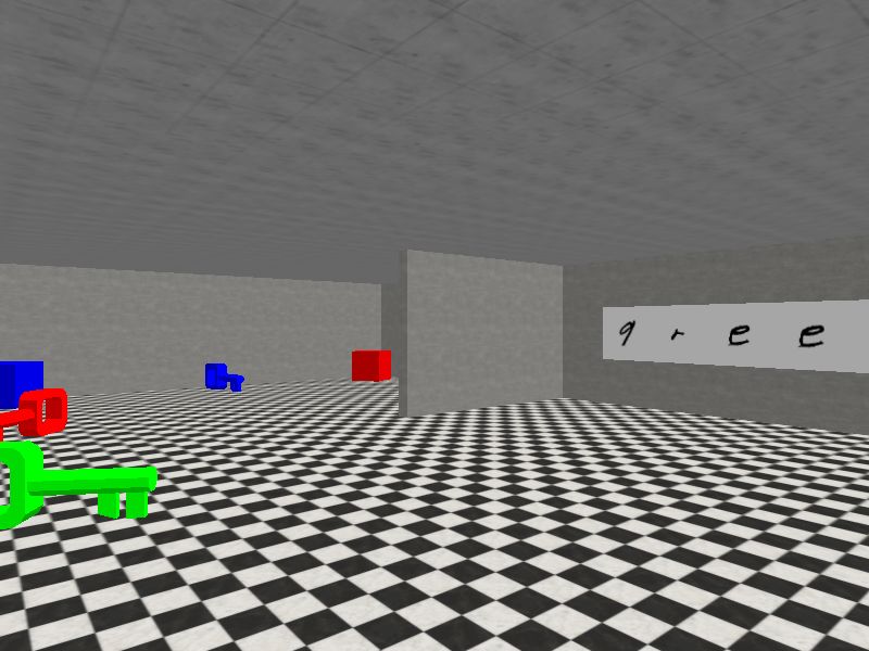
6.2 S PARSE -R EWARD 3D V ISUAL NAVIGATION
We conclude with a challenging benchmark testing both
sophisticated exploration and scalability to pixel inputs. We
modify a benchmark from Kamienny et al. (2020) to increase
both the exploration and scalability challenge by including
more objects and a visual sign, illustrated in Figure 7. In
the 3 different problems, the sign on the right says “blue”,
“red” or “green.” The goals specify whether the agent should
collect the key or block. The agent receives +1 reward for
collecting the correct object (color specified by the sign,
shape specified by the goal), -1 reward for the wrong object,
and 0 reward otherwise. The agent begins the episode on Figure 7: 3D Visual Navigation. The agent
the far side of the barrier and must walk around the barrier must read the sign to determine what col-
to visually “read” the sign. The agent’s observations are ored object to go to.
80 × 60 RGB images and its actions are to rotate left or right, move forward, or end the episode.
D REAM is the only method that learns to read the sign and achieve reward (Figure 6 right). All end-to-
end approaches get stuck in local optima, where they do not learn to read the sign and hence stay away
from all the objects, in fear of receiving negative reward. This achieves close to 0 returns, consistent
with the results in Kamienny et al. (2020). As before, P EARL -UB cannot learn optimal exploration.
7 C ONCLUSION
In summary, this work identifies a chicken-and-egg problem that end-to-end meta-RL approaches
suffer from, where learning good exploitation requires already having learned good exploration and
vice-versa. This creates challenging local optima, since typically neither exploration nor exploitation
is good at the beginning of meta-training. We show that appropriately leveraging simple one-hot
problem IDs allows us to break this cyclic dependency with D REAM. Consequently, D REAM has
strong empirical performance on meta-RL problems requiring complex exploration, as well as
substantial theoretical sample complexity improvements in the tabular setting. Though prior works
also leverage the problem ID and use decoupled objectives that avoid the chicken-and-egg problem, no
other existing approaches can recover optimal exploration empirically and theoretically like D REAM.
8
Under review as a conference paper at ICLR 2021

R EFERENCES
R. Agarwal, C. Liang, D. Schuurmans, and M. Norouzi. Learning to generalize from sparse and
  underspecified rewards. arXiv preprint arXiv:1902.07198, 2019.
M. Andrychowicz, M. Denil, S. Gomez, M. W. Hoffman, D. Pfau, T. Schaul, B. Shillingford, and
 N. D. Freitas. Learning to learn by gradient descent by gradient descent. In Advances in neural
 information processing systems, pp. 3981–3989, 2016.
D. Barber and F. V. Agakov. The IM algorithm: a variational approach to information maximization.
  In Advances in neural information processing systems, 2003.
S. Bengio, Y. Bengio, J. Cloutier, and J. Gecsei. On the optimization of a synaptic learning rule. In
   Preprints Conf. Optimality in Artificial and Biological Neural Networks, volume 2, 1992.
Y. Bengio, S. Bengio, and J. Cloutier. Learning a synaptic learning rule. In IJCNN-91-Seattle
  International Joint Conference on Neural Networks, volume 2, pp. 969–969, 1991.
M. Chevalier-Boisvert. Gym-Miniworld environment for openai gym. https://github.com/
 maximecb/gym-miniworld, 2018.
R. Dorfman and A. Tamar. Offline meta reinforcement learning. arXiv preprint arXiv:2008.02598,
  2020.
Y. Duan, J. Schulman, X. Chen, P. L. Bartlett, I. Sutskever, and P. Abbeel. RL2 : Fast reinforcement
   learning via slow reinforcement learning. arXiv preprint arXiv:1611.02779, 2016.
B. Eysenbach, A. Gupta, J. Ibarz, and S. Levine. Diversity is all you need: Learning skills without a
  reward function. arXiv preprint arXiv:1802.06070, 2018.
R. Fakoor, P. Chaudhari, S. Soatto, and A. J. Smola.              Meta-Q-learning.      arXiv preprint
  arXiv:1910.00125, 2019.
C. Finn, P. Abbeel, and S. Levine. Model-agnostic meta-learning for fast adaptation of deep networks.
  In International Conference on Machine Learning (ICML), 2017.
K. Gregor, D. J. Rezende, and D. Wierstra.             Variational intrinsic control.   arXiv preprint
  arXiv:1611.07507, 2016.
A. Gupta, R. Mendonca, Y. Liu, P. Abbeel, and S. Levine. Meta-reinforcement learning of structured
  exploration strategies. In Advances in Neural Information Processing Systems (NeurIPS), pp. 5302–
  5311, 2018.
S. Gurumurthy, S. Kumar, and K. Sycara. Mame: Model-agnostic meta-exploration. arXiv preprint
   arXiv:1911.04024, 2019.
T. Hiraoka, T. Imagawa, V. Tangkaratt, T. Osa, T. Onishi, and Y. Tsuruoka. Meta-model-based meta-
   policy optimization. arXiv preprint arXiv:2006.02608, 2020.
S. Hochreiter, A. S. Younger, and P. R. Conwell. Learning to learn using gradient descent. In
  International Conference on Artificial Neural Networks (ICANN), pp. 87–94, 2001.
R. Houthooft, X. Chen, Y. Duan, J. Schulman, F. D. Turck, and P. Abbeel. Vime: Variational
  information maximizing exploration. In Advances in Neural Information Processing Systems
  (NeurIPS), pp. 1109–1117, 2016.
R. Houthooft, Y. Chen, P. Isola, B. Stadie, F. Wolski, O. J. Ho, and P. Abbeel. Evolved policy gradients.
  In Advances in Neural Information Processing Systems (NeurIPS), pp. 5400–5409, 2018.
J. Humplik, A. Galashov, L. Hasenclever, P. A. Ortega, Y. W. Teh, and N. Heess. Meta reinforcement
   learning as task inference. arXiv preprint arXiv:1905.06424, 2019.
L. P. Kaelbling, M. L. Littman, and A. R. Cassandra. Planning and acting in partially observable
  stochastic domains. Artificial intelligence, 101(1):99–134, 1998.

                                                   9
Under review as a conference paper at ICLR 2021

P. Kamienny, M. Pirotta, A. Lazaric, T. Lavril, N. Usunier, and L. Denoyer. Learning adaptive
   exploration strategies in dynamic environments through informed policy regularization. arXiv
   preprint arXiv:2005.02934, 2020.
S. Kapturowski, G. Ostrovski, J. Quan, R. Munos, and W. Dabney. Recurrent experience replay
   in distributed reinforcement learning. In International Conference on Learning Representations
  (ICLR), 2019.
R. Mendonca, A. Gupta, R. Kralev, P. Abbeel, S. Levine, and C. Finn. Guided meta-policy search. In
  Advances in Neural Information Processing Systems (NeurIPS), pp. 9653–9664, 2019.
N. Mishra, M. Rohaninejad, X. Chen, and P. Abbeel. A simple neural attentive meta-learner. arXiv
  preprint arXiv:1707.03141, 2017.
V. Mnih, K. Kavukcuoglu, D. Silver, A. A. Rusu, J. Veness, M. G. Bellemare, A. Graves, M. Ried-
   miller, A. K. Fidjeland, G. Ostrovski, et al. Human-level control through deep reinforcement
   learning. Nature, 518(7540):529–533, 2015.
A. Nagabandi, I. Clavera, S. Liu, R. S. Fearing, P. Abbeel, S. Levine, and C. Finn. Learning to
  adapt in dynamic, real-world environments through meta-reinforcement learning. arXiv preprint
  arXiv:1803.11347, 2018.
D. K. Naik and R. J. Mammone. Meta-neural networks that learn by learning. In [Proceedings 1992]
  IJCNN International Joint Conference on Neural Networks, volume 1, pp. 437–442, 1992.
K. Rakelly, A. Zhou, D. Quillen, C. Finn, and S. Levine. Efficient off-policy meta-reinforcement
  learning via probabilistic context variables. arXiv preprint arXiv:1903.08254, 2019.
J. Rothfuss, D. Lee, I. Clavera, T. Asfour, and P. Abbeel. Promp: Proximal meta-policy search. arXiv
   preprint arXiv:1810.06784, 2018.
D. Russo, B. V. Roy, A. Kazerouni, I. Osband, and Z. Wen. A tutorial on thompson sampling. arXiv
  preprint arXiv:1707.02038, 2017.
S. Sæmundsson, K. Hofmann, and M. P. Deisenroth. Meta reinforcement learning with latent variable
   gaussian processes. arXiv preprint arXiv:1803.07551, 2018.
A. Santoro, S. Bartunov, M. Botvinick, D. Wierstra, and T. Lillicrap. One-shot learning with memory-
  augmented neural networks. arXiv preprint arXiv:1605.06065, 2016.
J. Schmidhuber. Evolutionary principles in self-referential learning, or on learning how to learn: the
   meta-meta-... hook. PhD thesis, Technische Universität München, 1987.
B. Stadie, G. Yang, R. Houthooft, P. Chen, Y. Duan, Y. Wu, P. Abbeel, and I. Sutskever. The
  importance of sampling inmeta-reinforcement learning. In Advances in Neural Information
  Processing Systems (NeurIPS), pp. 9280–9290, 2018.
W. R. Thompson. On the likelihood that one unknown probability exceeds another in view of the
  evidence of two samples. Biometrika, 25(3):285–294, 1933.
S. Thrun and L. Pratt. Learning to learn. Springer Science & Business Media Springer Science &
   Business Media, 2012.
L. van der Maaten and G. Hinton. Visualizing data using t-SNE. Journal of machine learning
  research, 9(0):2579–2605, 2008.
H. van Hasselt, A. Guez, and D. Silver. Deep reinforcement learning with double Q-learning. In
  Association for the Advancement of Artificial Intelligence (AAAI), volume 16, pp. 2094–2100, 2016.
J. X. Wang, Z. Kurth-Nelson, D. Tirumala, H. Soyer, J. Z. Leibo, R. Munos, C. Blundell, D. Kumaran,
   and M. Botvinick. Learning to reinforcement learn. arXiv preprint arXiv:1611.05763, 2016a.
Z. Wang, T. Schaul, M. Hessel, H. V. Hasselt, M. Lanctot, and N. D. Freitas. Dueling network
  architectures for deep reinforcement learning. In International Conference on Machine Learning
  (ICML), 2016b.

                                                 10
Under review as a conference paper at ICLR 2021
D. Warde-Farley, T. V. de Wiele, T. Kulkarni, C. Ionescu, S. Hansen, and V. Mnih. Unsupervised
control through non-parametric discriminative rewards. arXiv preprint arXiv:1811.11359, 2018.
Y. Yang, K. Caluwaerts, A. Iscen, J. Tan, and C. Finn. Norml: No-reward meta learning. In
Proceedings of the 18th International Conference on Autonomous Agents and MultiAgent Systems,
pp. 323–331, 2019.
T. Yu, D. Quillen, Z. He, R. Julian, K. Hausman, C. Finn, and S. Levine. Meta-world: A benchmark
and evaluation for multi-task and meta reinforcement learning. arXiv preprint arXiv:1910.10897,
2019.
J. Zhang, J. Wang, H. Hu, Y. Chen, C. Fan, and C. Zhang. Learn to effectively explore in context-
based meta-RL. arXiv preprint arXiv:2006.08170, 2020.
A. Zhou, E. Jang, D. Kappler, A. Herzog, M. Khansari, P. Wohlhart, Y. Bai, M. Kalakrishnan,
S. Levine, and C. Finn. Watch, try, learn: Meta-learning from demonstrations and reward. arXiv
preprint arXiv:1906.03352, 2019a.
W. Zhou, L. Pinto, and A. Gupta. Environment probing interaction policies. arXiv preprint
arXiv:1907.11740, 2019b.
L. Zintgraf, K. Shiarlis, M. Igl, S. Schulze, Y. Gal, K. Hofmann, and S. Whiteson. Varibad: A very
good method for bayes-adaptive deep RL via meta-learning. arXiv preprint arXiv:1910.08348,
2019.
11Under review as a conference paper at ICLR 2021
A D REAM T RAINING D ETAILS
Algorithm 1 summarizes a practical algorithm for training D REAM. Unlike end-to-end approaches,
we choose not to make πθtask recurrent for simplicity, and only condition on z and the current state s.
We parametrize the policies as deep dueling double-Q networks (Wang et al., 2016b; van Hasselt
et al., 2016), with exploration Q-values Q̂exp (s, τ exp , a; φ) parametrized by φ (and target network
parameters φ0 ) and exploitation Q-values Q̂task (s, z, a; θ) parametrized by θ (and target network
parameters θ0 ). We train on trials with one exploration and one exploitation episode, but can test on
arbitrarily many exploitation episodes, as the exploitation policy acts on each episode independently
(i.e. it does not maintain a hidden state across episodes). Using the choices for Fψ and qω in
Section 4.3, training proceeds as follows.
We first sample a new problem for the trial and roll-out the exploration policy, adding the roll-out to a
replay buffer (lines 7-9). Then, we roll-out the exploitation policy, adding the roll-out to a separate
replay buffer (lines 10-12). We train the exploitation policy on both stochastic encodings of the
problem ID N (fψ (µ), ρ2 I) and on encodings of the exploration trajectory gω (τ exp ).
Next, we sample from the replay buffers and update the parameters. First, we sample
(st , at , st+1 , µ, τ exp )-tuples from the exploration replay buffer and perform a normal DDQN update
on the exploration Q-value parameters φ using rewards computed from the decoder (lines 13-15).
Concretely, we minimize the following standard DDQN loss function w.r.t., the parameters φ, where
the rewards are computed according to Equation 4:
2
exp exp exp exp exp 0
Lexp (φ) = E Q̂ (st , τ:t−1 , at ; φ) − (rt + γ Q̂ (st+1 , [τ:t−1 ; at ; st ], aDDQN ; φ ) ,
2
2 2
where rtexp
= fψ (µ) − gω (τ:texp ) 2 − fψ (µ) − gω (τ:t−1 exp
) 2 −c
exp
and aDDQN = arg max Q̂exp (st+1 , [τ:t−1 ; at ; st ]; φ).
a
We perform a similar update with the exploitation Q-value parameters (lines 16-18). We sample
(s, a, r, s0 , µ, τ exp )-tuples from the exploitation replay buffer and perform two DDQN updates, one
from the encodings of the exploration trajectory and one from the encodings of the problem ID by
minimizing the following losses:
2
task exp task 0 exp 0
Ltask-traj (θ, ω) = E Q̂ (s, gω (τ ), a; θ) − (r + Q̂ (s , gω (τ ), atraj ; θ )
0 ,
2
2
and Ltask-id (θ, ψ) = E Q̂task (s, fψ (µ), a; θ) − (r + Q̂task (s0 , fψ0 (µ), aprob ; θ0 ) ,
2
task 0 exp task 0
where atraj = arg max Q̂ (s , gω (τ ), a; θ) and aprob = arg max Q̂ (s , fψ (µ), a; θ).
a a
Finally, from the same exploitation replay buffer samples, we also update the problem ID embedder
to enforce the information bottleneck (line 19) and the decoder to approximate the true conditional
distribution (line 20) by minimizing the following losses respectively:
h i
2
Lbottleneck (ψ) = Eµ min (kfψ (µ)k2 , K)
" #
exp 2
X
and Ldecoder (ω) = Eτ exp fψ (µ) − gω (τ:t ) 2 .
t
2
Since the magnitude kfψ (µ)k2
partially determines the scale of the reward, we add a hyperparameter
K and only minimize the magnitude when it is larger than K. Altogether, we minimize the following
loss:
L(φ, θ, ω, ψ) = Lexp (φ) + Ltask-traj (θ, ω) + Ltask-id (θ, ψ) + Lbottleneck (ψ) + Ldecoder (ω).
As is standard with deep Q-learning (Mnih et al., 2015), instead of sampling from the replay buffers
and updating after each episode, we sample and perform all of these updates every 4 timesteps. We
periodically update the target networks (lines 21-22).
12Under review as a conference paper at ICLR 2021
Algorithm 1 D REAM DDQN
1: Initialize exploitation replay buffer Btask-id = {} and exploration replay buffer Bexp = {}
2: Initialize exploitation Q-value Q̂task parameters θ and target network parameters θ0
3: Initialize exploration Q-value Q̂exp parameters φ and target network parameters φ0
4: Initialize problem ID embedder fψ parameters ψ and target parameters ψ 0
5: Initialize trajectory embedder gω parameters ω and target parameters ω 0
6: for trial = 1 to max trials do
7: Sample problem µ ∼ p(µ), defining MDP hS, A, Rµ , Tµ i
8: Roll-out -greedy exploration policy Q̂exp (st , τ:texp , at ; φ), producing trajectory τ exp = (s0 , a0 , . . . , sT ).
9: Add tuples to the exploration replay buffer Bexp = Bexp ∪ {(st , at , st+1 , µ, τ exp )}t .
10: Randomly select between embedding z ∼ N (fψ (µ), ρ2 I) and z = gω (τ exp ).
11: Roll-out -greedy exploitation policy Q̂task (st , z, at ; θ), producing trajectory (s0 , a0 , r0 , . . .) with
rt = Rµ (st+1 ).
12: Add tuples to the exploitation replay buffer Btask-id = Btask-id ∪ {(st , at , rt , st+1 , µ, τ exp )}t .
13: Sample batches of (st , at , st+1 , µ, τ exp ) ∼ Bexp from exploration replay buffer.
2 2
14: Compute reward rtexp = kfψ (µ) − gω (τ:texp )k2 − fψ (µ) − gω (τ:t−1 exp
) 2 − c (Equation 4).
exp
15: Optimize φ with DDQN update with tuple (st , at , rt , st+1 ) with Lexp (φ)
16: Sample batches of (s, a, r, s0 , µ, τ exp ) ∼ Btask-id from exploitation replay buffer.
17: Optimize θ and ω with DDQN update with tuple ((s, τ exp ), a, r, (s0 , τ exp )) with Ltask-traj (θ, ω)
18: Optimize θ and ψ with DDQN update with tuple ((s, µ), a, r, (s0 , µ)) with Ltask-id (θ, ψ)
19: Optimize ψ on Lbottleneck (ψ) = ∇ψ min(kfψ (µ)k22 , K)
2
Optimize ω on Ldecoder (ω) = ∇ω t kfψ (µ) − gω (τ:texp )k2 (Equation 3)
P
20:
21: if trial ≡ 0 (mod target freq) then
22: Update target parameters φ0 = φ, θ0 = θ, ψ 0 = ψ, ω 0 = ω
23: end if
24: end for
B E XPERIMENT D ETAILS
B.1 P ROBLEM D ETAILS
Distracting bus / map. Riding each of the four colored buses teleports the agent to near one of
the green goal locations in the corners. In different problems, the destinations of the colored buses
change, but the bus positions and their destinations are fixed within each problem. Additionally, in
the distracting bus domain, the problem ID also encodes the destinations of the gray buses, which are
permutations of the four gray locations on the midpoints of the sides. More precisely, the problem ID
µ ∈ {0, 1, . . . , 4! × 4! = 576} encodes both the permutation of the colored helpful bus
µdestinations,
indexed as µ (mod 4!) and the permutation of the gray unhelpful bus destinations as 4! . We hold
23
out most of the problem IDs during meta-training ( 24 × 576 = 552 are held-out for meta-training).
In the map domain, the problem µ is an integer representing which of the 4! permutations of the four
green goal locations the colored buses map to. The states include an extra dimension, which is set to
0 when the agent is not at the map, and is set to this integer value µ when the agent is at the map.
Figure 8 displays three such examples.
Cooking. In different problems, the (color- (a) (b) (c)
coded) fridges contain 1 of 4 different ingre-
dients. The ingredients in each fridge are un-
known until the goes to the fridge and uses the
pickup action. Figure 9 displays three example
problems. The problem ID µ is an integer be- agent fridge (ingredients) pot
tween 0 and 43 , where µ = 42 a + 4b + c indi-
cates that the top right fridge has ingredient a,
the middle fridge has ingredient b and the bot- Figure 9: Three example cooking problems. The con-
tom right fridge has ingredient c. tents of the fridges (color-coded) are different in differ-
ent problems.
13Under review as a conference paper at ICLR 2021
(a) (b) (c)
agent map unhelpful bus stop bus goal
Figure 8: Examples of different distracting bus and map problems. (a) An example distracting bus problem.
Though all unhelpful distracting buses are drawn in the same color (gray), the destinations of the gray buses are
fixed within a problem. (b) Another example distracting bus problem. The destinations of the helpful colored
buses are a different permutation (the orange and green buses have swapped locations). This takes on permutation
3 ≡ µ (mod 4!),instead of 1. The unhelpful gray buses are also a different permutation (not shown), taking on
µ
permutation 5 = 4! . (c) An example map problem. Touching the map reveals the destinations of the colored
buses, by adding µ to the state observation.
The goals correspond to a recipe of placing the two correct ingredients in the pot in the right order.
Goals are tuples (a, b), which indicate placing ingredient a in the pot first, followed by ingredient
b. In a given problem, we only sample goals involving the recipes actually present in that problem.
During meta-training, we hold out a randomly selected problem µ = 11.
We use the following reward function Rµ . The agent receives a per timestep penalty of −0.1 reward
and receives +0.25 reward for completing each of the four steps: (i) picking up the first ingredient
specified by the goal; (ii) placing the first ingredient in the pot; (iii) picking up the second ingredient
specified by the goal; and (iv) placing the second ingredient in the pot. To prevent the agent from
gaming the reward function, e.g., by repeatedly picking up the first ingredient, dropping the first
ingredient anywhere but in the pot yields a penalty of −0.25 reward, and similarly for all steps. To
encourage efficient exploration, the agent also receives a penalty of −0.25 reward for picking up the
wrong ingredient.
Cooking without goals. While we evaluate on goal-conditioned benchmarks to deepen the explo-
ration challenge, forcing the agent to discover all the relevant information for any potential goal,
many standard benchmarks (Finn et al., 2017; Yu et al., 2019) don’t involve goals. We therefore in-
clude a variant of the cooking task, where there are no goals. We simply concatenate the goal (recipe)
to the problem ID µ. Additionally, we modify the rewards so that picking up the second ingredient
yields +0.25 and dropping it yields −0.25 reward, so that it is possible to infer the recipe from the
rewards. Finally, to make the problem harder, the agent cannot pick up new ingredients unless its
inventory is empty (by using the drop action), and we also increase the number of ingredients to 7.
The results are in Section B.2.
Sparse-reward 3D visual navigation. We implement this domain in Gym MiniWorld (Chevalier-
Boisvert, 2018), where the agent’s observations are 80 × 60 × 3 RGB arrays. There are three problems
µ = 0 (the sign says “blue”), µ = 1 (the sign says “red”), and µ = 2 (the sign says “green”). There
are two goals, represented as 0 and 1, corresponding to picking up the key and the box, respectively.
The reward function Aµ (s, i) is +1 for picking up the correct colored object (according to µ) and the
correct type of object (according to the goal) and −1 for picking up an object of the incorrect color or
type. Otherwise, the reward is 0. On each episode, the agent begins at a random location on the other
side of the barrier from the sign.
B.2 A DDITIONAL R ESULTS
14You can also read