Nvidia's Stock Returns Prediction Using Machine Learning Techniques for Time Series Forecasting Problem
←
→
Page content transcription
If your browser does not render page correctly, please read the page content below
ISSN: 2543-6821 (online)
                  Journal homepage: http://ceej.wne.uw.edu.pl

                  Marcin Chlebus, Michał Dyczko,
                  Michał Woźniak

Nvidia’s Stock Returns Prediction
Using Machine Learning
Techniques for Time Series
Forecasting Problem
                  To cite this article

                  Chlebus, M., Dyczko, M., Woźniak, M. (2021). Nvidia’s Stock Returns
                  Prediction Using Machine Learning Techniques for Time Series
                  Forecasting Problem. Central European Economic Journal, 8(55), 44-62.

                  DOI: 10.2478/ceej-2021-0004

                  To link to this article: https://doi.org/10.2478/ceej-2021-0004

 Open Access. © 2021 M. Chlebus, M. Dyczko, M. Woźniak, published by Sciendo.
 This work is licensed under the Creative Commons Attribution-NonCommercial-NoDerivatives 4.0 License.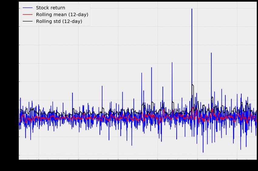
Marcin Chlebus
              Faculty of Economic Sciences, Division of Quantitative Finance, University of Warsaw,
              Warszawa, Poland
              corresponding author: mchlebus@wne.uw.edu.pl

              Michał Dyczko
              Faculty of Mathematics and Computer Science, Warsaw University of Technology, Warszawa,
              Poland

              Michał Woźniak
              Faculty of Economic Sciences, University of Warsaw, Warszawa, Poland

Nvidia’s Stock Returns Prediction Using Machine Learning
Techniques for Time Series Forecasting Problem

Abstract
Statistical learning models have profoundly changed the rules of trading on the stock exchange. Quantitative analysts
try to utilise them predict potential profits and risks in a better manner. However, the available studies are mostly
focused on testing the increasingly complex machine learning models on a selected sample of stocks, indexes etc.
without a thorough understanding and consideration of their economic environment. Therefore, the goal of the
article is to create an effective forecasting machine learning model of daily stock returns for a preselected company
characterised by a wide portfolio of strategic branches influencing its valuation. We use Nvidia Corporation stock
covering the period from 07/2012 to 12/2018 and apply various econometric and machine learning models, considering a
diverse group of exogenous features, to analyse the research problem. The results suggest that it is possible to develop
predictive machine learning models of Nvidia stock returns (based on many independent environmental variables)
which outperform both simple naïve and econometric models. Our contribution to literature is twofold. First, we
provide an added value to the strand of literature on the choice of model class to the stock returns prediction problem.
Second, our study contributes to the thread of selecting exogenous variables and the need for their stationarity in the
case of time series models.

Keywords
machine learning | nvidia | stock returns | technical analysis | fundamental analysis

JEL Codes
C02, C32, C40, G12

1 Introduction                                               of fundamental analysis, technical analysis and
                                                             behaviour analysis with good results. But, at the same
In recent years, researchers have attempted to find          time, the last decade was a renaissance of supervised
novel and unbiased theoretical foundations that would        machine learning algorithms that are used in time
be useful for understanding the behaviour of financial       series prediction problems in such areas as energetics
markets. The hypothesis that was considered as a             (Chou & Tran, 2018), finance (Abe & Nakayama, 2018),
breakthrough for the academic world in the above-            logistics (Laptev, Yosinski, Li & Smyl, 2017) etc. It
mentioned field is ‘The Adaptive Markets Hypothesis’         seems that the combination of The Adaptive Markets
(Lo, 2004). It means the ability to use the achievements     Hypothesis and Machine Learning models for time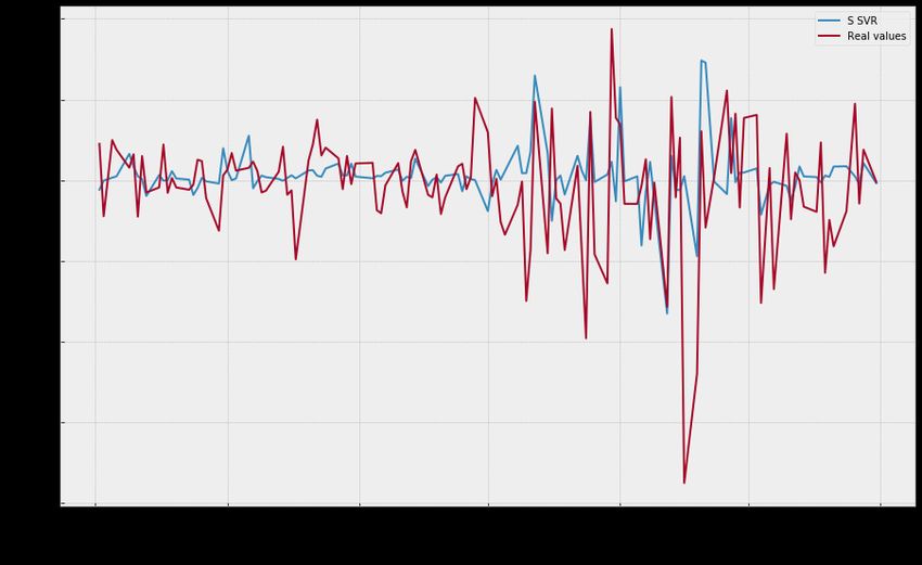
CEEJ • 8(55) • 2021 • pp. 44-62 • ISSN 2543-6821 • DOI: 10.2478/ceej-2021-0004        46

series can produce tangible results in stock returns        ranking-based ensemble models perform better than
forecasting.                                                singular ones? and (4) Are the categories of variables
                                                            suggested in literature significant?
    The main purpose of this study is to forecast the
daily stock returns of Nvidia Corporation company                The structure of this paper was composed as
quoted on the Nasdaq Stock Market effectively, using        follows. The second part dealt with the literature
numerous exogenous explanatory variables. The               review. The third part was devoted to the materials
most important problems standing to be focussed             and methodology used in research. The fourth
by researchers are statistical specificity of rates of      part presented the results of empirical research and
return i.e. as a time series they can be a white noise      answers to the hypotheses. The last part contained a
(Hill & Motegi, 2019), necessity of applying many           summary of the work and conclusions.
atypical machine learning methods to handle the
influence of the time factor (Bontempi, Taieb &
Borgne, 2012) and the lack of publications constituting     2. Literature Review
a benchmark in terms of regression problem.
The Nvidia Corporation is selected intentionally            Studies focussed to stock returns prediction in
based on economic sense because of its unique and           regression field using statistical learning techniques
complex cross-sectoral structure, including games,          is quite skimpy, especially as far as one-day-ahead
deep learning and cryptocurrency market. From a             forecast is concerned. Authors who made significant
modelling perspective, it gives us the possibility to use   contributions to this subject are Abe and Nakayama
many exogenous features that can have a significant         (2018). Their study examined performance of DNN,
impact on the endogenous variable − rate of return.         RF and SVM models in predicting one-month-ahead
Moreover, one can observe that Nvidia`s stock price         stock returns in the cross-section on the Japanese
changes rapidly between October 2018 and December           stock market. Moreover, they also applied weighted
2018. It is interesting to analyse whether the models       ensemble method. The experimental results indicate
are able to detect these fluctuations and predict stock     that Deep Neural Networks and weighted ensembling
returns well.                                               show great potential at stock returns forecast. Rather,
                                                            Agarwal and Sastry (2015) proposed hybrid model
    As mentioned above, the models used in this article     for prediction of stock returns. The proposed model
are based on variables from various sources namely          is constituted of RNN, ARMA and Holt model. The
fundamental analysis of Nvidia Corporation, technical       results obtained by the researchers indicated better
analysis of Nvidia stock prices, behaviour analysis from    accuracy of the hybrid model compared to single
Google Trends data, etc. The research period spread         realizations of the above-mentioned approaches.
over the years 02/07/2012–31/12/2018 and the period         Another example is provided by Pai and Lin (2005)
is divided into training set (02/07/2012–29/06/2018)        who tried to predict stock price using ARIMA,
and testing set (02/07/2018–31/12/2018). This is done       SVR and hybrid of these models (complementary
because of the desire to test the performance of models     dependence: SVR was specified to predict residuals of
in this particular period of time. The algorithms           ARIMA, and therefore minimise forecast error) on ten
that will be applied to this data materialised from         stocks basing on daily closing prices. They obtained
two types of frameworks – machine learning: SVR,            promising and potential capability of the hybrid model
KNN, XGBoost, LightGBM and LSTM Networks;                   to forecast time series. In their case, simple average
and econometric methods: ARMA and ARMAX.                    of two models does not gain any significant impact.
Further, we tested ranking-based ensemble model on          Adebiyi, Adewunmi and Ayo (2014) applied ANN and
the above-mentioned algorithms.                             ARIMA on daily stock data from NYSE and examined
     The main hypothesis verified in this paper is          their performance. The empirical results presented the
whether it is possible to construct predictive machine      superiority of neural networks model over ARIMA
learning model of Nvidia’s daily stock returns, which       model. It is also worth mentioning interesting works
can outperform both simple naive and econometric            on classification problem of stock prices. Zheng and
models. The additional research questions are (1)           Jin (2017) analysed the results of logistic regression,
will models cope with the market fluctuations that          Bayesian network, LSTM and SVM on daily Microsoft
began in October 2018?, (2) Do models based on              stock prices, along with technical indicators. The
stationary variables perform better than models based       results indicated that they could achieve a correct
on stationary and non-stationary variables?, (3) Will       prediction of the price trends at level of 70%. SVM
CEEJ • 8(55) • 2021 • pp. 44-62 • ISSN 2543-6821 • DOI: 10.2478/ceej-2021-0004 47
gained the best score. Chen, Zhou and Dai (2015) and Ali (2018) divided the variables into categories so
successfully applied LSTM to forecast changes in that they describe the company as a whole: liquidity
stock returns for China stock market in Shanghai (current liquidity), market value (price/profit, EPS),
and Shenzhen. Moreover, they showed that additional profitability (ROA), indebtedness (general debt). Their
exogenous variables such as technical analysis data research for the emerging Pakistani stock exchange
increase the predictive power of the model. Milosevic showed that the variables ROA (positive coefficient)
(2016) forecasted long-term stock price movement and Price/Earnings (positive coefficient) were
using RF, logistic regression and Bayesian networks. highly significant in modelling rates. The remaining
In this study, the author gathered quarterly stock variables were irrelevant or showed illogical
prices from over 1700 stocks together with data from dependencies. The use of variables from technical
fundamental analysis. He showed that RF is the best analysis is slightly less systematised in academic
one and it also provided the most appropriate set of literature than variables from fundamental analysis.
fundamental indicators. Stanković, Marković and Stojanović (2015) examined
the effectiveness of using three technical analysis
Based on the achievements of researchers in indicators: EMA (Exponential Moving Average),
the field of stock returns forecasting, following MACD (Moving Average Convergence-Divergence)
econometric models will be used in this article: and RSI (Relative Strength Index) to predict stock
ARIMA developed by Whittle (1951) and popularised returns on selected stock exchanges in the countries of
by Box and Jenkins (1970), ARIMAX which gives former Yugoslavia. According to their research, EMA
possibility to extend ARIMA model with additional and MACD produced the best performance, while
exogenous variables. Nonlinear supervised machine RSI was unable to predict rates of return as expected.
learning models applied in this research are: SVR Hybrid models with variables from technical and
created by Vapnik, Drucker, Burges, Kaufman and fundamental analysis were also well-described in
Smola (1997) and KNN designed by Altman (1992). literature. Beyaz, Tekiner, Zeng and Keane (2018)
Models from the same category as stated above and conducted an experiment based on forecasting the
based on boosted decision trees are XGBoost developed share prices of companies from the S&P index in time
by Chen and Guestring (2016) and LightGBM created windows: 126 and 252 days. Their analysis showed
by Ke, Meng, Finley, Wang and Chen (2017). During that hybrid models work better than single models.
the research, RNN in LSTM architecture constructed They also investigated the significance of variables
by Hochreiter and Schmidhuber (1997) was also in the hybrid approach (division into three tiers). The
deployed. To conduct ensembling, a Model Ranking highest, which means the most effective tier, consists
Based Selective Ensemble Approach powered by paper of ATR and EPS. Emir, Dincer and Timor (2012)
of Adhikari, Verma and Khandelwal (2015) was used. conducted research on the specificity of the Turkish
A particularly important part of the entire analysis stock exchange. They created a model that ranked ten
is the collection of variables from various thematic in the most profitable companies on the market. They
classes i.e.: fundamental analysis, technical analysis, used a hybrid approach, which turned out to be much
behavioural analysis, expert indicators of Nvidia- more effective than single models. The variables that
related markets. Undoubtedly, the best described in turned out to be significant in the analysis are: Price
the literature is the selection of variables from the per Book Value, ROE, CCI and RSI.
fundamental analysis to the problem of prediction of In the literature, the behavioural analysis of
stock prices and stock returns. Mahmoud and Sakr speculators is divided into sentiment analysis and
(2012) showed that fundamental variables explaining analysis of the popularity of search terms on the
issues such as profitability, solvency, liquidity and Internet. This paper is focussed on the second
operational efficiency are helpful in creating effective approach. Ahmed, Asif, Hina and Muzammil (2017)
investment strategies. Zeytinoglu, Akarim and collected data from Google Trends to capture the
Celik (2012) showed that following factors are good relationship between online searches and political
predictors of stock returns in their study on the and business events. They used this knowledge to
Turkish insurance market: Price/Profit, Earnings predict the ups and downs of the Pakistan Stock
per Share and Price to Book Ratio. Hatta (2012), in Exchange Index 100, quantifying the semantics of
his research, found that Earnings Per Share has a the international market. Their research shows that
positive effect on the rate of return and is negatively these variables have good prognostic properties. Preis,
correlated with the Debt to Equity Ratio. Muhammad Moat and Stanley (2013) used Google Trends data toCEEJ • 8(55) • 2021 • pp. 44-62 • ISSN 2543-6821 • DOI: 10.2478/ceej-2021-0004 48
predict the value of Dow Jones Industrial Average and indexes of S&P500 and NASDAQ-100. The stocks
Index. They claimed that these features provide some include entities that are competitors of Nvidia and
insight into future trends in the behaviour of traders their close business partners. On the other hand, the
and can be good factor in the decision-making process indices show the general market situation. They were
for investors. In addition, the Nvidia Annual Financial collected from Yahoo Finance.
Report (2018) legitimises the need to collect indicators
Nvidia’s fundamental analysis features origins
linked to Nvidia related markets such as deep learning,
from the balance sheet and are available on the
games and crypto currency.
Bloomberg Terminal. Such variables are:
Yang and Shahabi (2005) show that not only
• Profitability ratios: Return on Equity, Return on
model and variables selection are important, but also
Assets, Gross Margin, Operating Margin, Return
the feature engineering. They performed several
on Investment, Earnings Before Interests and
classification experiments using correlation coefficient
Taxes Margin, Pre-Tax Profit Margin, Net Profit
techniques on four datasets and investigated how
Margin;
data stationarity influences forecast accuracy. The
results of their work indicate that one can obtain • Liquidity ratios: Currrent Ratio, Operating Cash
higher accuracy in prediction after differencing non- Flow per Share, Free Cash Flow per Share;
stationary data, while differencing stationary data • Debt ratios: Long-term Debt to Capital, Debt to
makes the forecast less accurate. The authors suggest Equity ratio;
that the test of stationarity and possible differencing • Efficiency Ratios: Asset turnover, Inventory
features is recommended pre-processing step. Turnover Ratio, Receivable Turnover, Days Sales
Ultimately, we need to emphasise that Nvidia stock Outstanding;
price dropped rapidly in 3rd quarter of 2018 by more • Market ratios: Earning per share, Price to book
than 30 per cent after the earning results presentation. value ratio, Book value per share, Price to Earnings
Experts (Abazovic, 2018; Eassa, 2018) associate this ratio;
fact to previous diminishment in crypto interest and
mining. This has led to severe demand decrease for
The behavioural analysis was based on a people’s
graphic processing units, which are Nvidia’s main
demand for information taken from the Internet,
product line useful in cryptocurrencies mining.
especially from the Google Search and Google
News. These data are available on the Google Trends
platform. It was decided to look for entries related to
3. Materials and Methods this study such as:
3.1 Dataset • Google search: Nvidia, Geforce, GTX, GPU,
AMD, Intel, Deep learning, Artificial intelligence,
Dataset preparation step was crucial in this research. Machine learning, Neural network, Data science,
After data pre-processing, dataset consists of more than Natural language processing, Fintech, Azure,
350 independent variables from various categories. AWS, Google Cloud, Tensorflow, PyTorch, Mxnet,
The data used in this paper belongs to the period Blockchain, Cryptocurrency, Bitcoin, Ethereum,
from 01/01/2012 to 31/12/2018. All information was Bitcoin miner, Cryptocurrency miner, Gaming,
collected in January 2019. E-sport, Battlefield, Just cause, Assassins Creed,
Hitman, Far cry, Final fantasy, Forza motorsport,
Call of duty, Witcher, Fallout, Gaming PC, Nvidia
shield, GTA, Python, Twitch;
3.1.1. Data sources
• Google news: Nvidia, GTX, GPU, AMD, Deep
The key variables among all others used in the learning, Artificial intelligence, Data science,
article are open price, close price, high price, low Fintech, AWS, Blockchain, Bitcoin, Ethereum,
price and volume for stocks of companies such as Gaming, E-sport, Battlefield, Just cause, Assassins
Nvidia Corporation (NVIDIA), Advanced Micro Creed, Hitman, Far cry, Final fantasy, Forza
Devices, Inc. (AMD), Bitcoin USD (BTC), Ubisoft motorsport, Call of duty, Witcher, Fallout,
Entertainment SA (UBSFY), Activision Blizzard Inc. Gaming PC.
(ATVI), Take-Two Interactive Software Inc. (TTWO)CEEJ • 8(55) • 2021 • pp. 44-62 • ISSN 2543-6821 • DOI: 10.2478/ceej-2021-0004 49
They were gathered from an area covering the Parabolic SAR – Extended, Triple Exponential
whole world. Moving Average, Triangular Moving Average,
Weighted Moving Average;
In order to capture how the Artificial Intelligence
market is developing, it was decided to use a proxy in • Momentum Indicators: Momentum,
the form of a number of scientific publications in the Commodity Channel Index, Relative Strength
field of statistics and machine learning published on Index, Williams’%R, Money Flow Index,
the Arxiv website. These data were collected using Directional Movement Index, Plus Directional
web-scraping. Movement, Percentage Price Oscillator, Aroon
Oscillator, Balance Of Power, Minus Directional
Driven by the need to use some gaming market Movement, Ultimate Oscillator, Average
data in this paper, the publication dates for the most Directional Movement Index, Average Directional
demanding PC video games were scrapped from Movement Index Rating, Absolute Price
game-debate.com along with average FPS that each Oscillator, Chande Momentum Oscillator, Minus
game scored on single set of software with GeForce Directional Indicator, Plus Directional Indicator,
GTX 1060 at 1080p resolution. Rate of change, Rate of change Percentage, Rate of
Our study also considered non-financial change ratio, Rate of change ratio 100 scale;
information published by Nvidia, which may influence • Volume Indicators: Chaikin A/D Line, On
the decisions of speculators. These variables are Balance Volume, Chaikin A/D Oscillator;
publication dates of various thematic articles on the • Volatility Indicators: Average True Range,
Nvidia Newsroom website, dates of the announcement Normalised Average True Range, True Range;
of new graphics cards and GPUs by Nvidia. Features • Price Transform: Average Price, Median Price,
were crawled respectively from Nvidia and Wikipedia Typical Price, Weighted Close Price;
pages.
• Cycle Indicators: Hilbert Transform – Dominant
Further, dataset was extended with such features Cycle Period, Hilbert Transform – Dominant
like day of a week, day of a year, month, quarter to Cycle Phase, Hilbert Transform – Trend vs Cycle
handle time series specificity of the research. Mode;
• Pattern Recognition: Two Crows, Three Black
Crows, Three Inside Up/Down, Three-Line
3.1.2. Feature preparation Strike, Three Outside Up/Down, Three Stars
Return ratios for: NVIDIA, BTC, UBSFY, ATVI, In The South, Three Advancing White Soldiers,
TTWO, BTC, S&P500, NASDAQ-100 were calculated Abandoned Baby, Advance Block, Belt-hold,
using the formula: Breakaway, Closing Marubozu, Concealing Baby
Swallow, Counterattack, Dark Cloud Cover, Doji,
Doji Star, Dragonfly Doji, Engulfing Pattern,
pricet − pricet −1
return ratio = . (1) Evening Doji Star, Evening Star, Up/Down-
pricet −1 gap side-by-side white lines, Gravestone Doji,
Hammer, Hanging Man, Harami Pattern, Harami
For the same variables, a 10-period rolling Cross Pattern, High-Wave Candle, Hikkake
variance was applied. Pattern, Modified Hikkake Pattern, Homing
Pigeon, Identical Three Crows, In-Neck Pattern,
Technical analysis of Nvidia prices was obtained
Inverted Hammer, Kicking, Kicking - bull/bear
using Open Source Technical Analysis Library (TA-
determined by the longer marubozu, Ladder
Lib). Depending on the technical indicator, a different
Bottom, Long Legged Doji, Long Line Candle,
set of Nvidia attributes (opening price, closing price,
Marubozu, Matching Low, Mat Hold, Morning
highest price, lowest price, volume) was used to
Doji Star, Morning Star, On-Neck Pattern, Piercing
generate a new variable. Gathered features are:
Pattern, Rickshaw Man, Rising/Falling Three
• Overlap Studies: Exponential Moving Average, Methods, Separating Lines, Shooting Star, Short
Double Exponential Moving Average, Hilbert Line Candle, Spinning Top, Stalled Pattern, Stick
Transform – Instantaneous Trendline, Kaufman Sandwich, Takuri, Tasuki Gap, Thrusting Pattern,
Adaptive Moving Average, Midpoint over period, Tristar Pattern, Unique 3 River, Upside Gap Two
Midpoint Price over period, Parabolic SAR, Crows, Upside/Downside Gap Three Methods;CEEJ • 8(55) • 2021 • pp. 44-62 • ISSN 2543-6821 • DOI: 10.2478/ceej-2021-0004 50
• Statistic Functions: Pearson’s Correlation to take this element into consideration. Moreover,
Coefficient, Linear Regression, Linear Regression scientists put strong emphasis on preventing data
Angle, Linear Regression Intercept, Linear leaks. Therefore, they analysed possible problems for
Regression Slope, Standard Deviation, Time each group of variables, e.g. the date of publication of
Series Forecast, Variance; financial statements (fundamental variables) or data
• Math Transform Functions: Vector Trigonometric scaling (Google Trends) and prepared the input data
ATan, Vector Ceil, Vector Trigonometric Cos, accordingly.
Vector Trigonometric Cosh, Vector Arithmetic Exp,
Vector Floor, Vector Log Natural, Vector Log10,
Vector Trigonometric Sin, Vector Trigonometric 3.2. General methodology of research
Sinh, Vector Square Root, Vector Trigonometric
Tan, Vector Trigonometric Tanh; In this paper, we tested performances of models based
on features from two categories namely all variables
• Math Operator Functions: CAPM Beta, Highest
(stationary and non-stationary) and only stationary
value over a specified period, Index of highest
variables. Thus, each model was built twice, but
value over a specified period, Lowest value over
methodology remains the same.
a specified period, Index of lowest value over a
specified period, Vector Arithmetic Mult, Vector The performance of each model was interpreted as
Arithmetic Substraction, Summation. Root Mean Squared Error (RMSE) score between its
predicted values and empirical values of stock returns.
The choice of this metric is implied by the fact that it
Factors mentioned above were calculated on the emphasises the importance of large individual errors.
assumption of default values of parameters in the What’s more, RMSE does not generate computational
software. problems due to lack of y in the denominator that
The Min-Max Scaler was applied to all variables could lead to a zero-division error in the stock return
from Google Trends and Google News, and newly problem. In addition, , the metrics Mean Absolute
generated data was included in the base dataset. Error (MAE) and Median Absolute Error (MedAE)
Hence, scaled and non-scaled Google variables were were considered to better understand and analyse the
taken into account. final results.
Data from Google Trends, Google News and game Moreover, we defined a simple naive model,
release dates had non-daily frequency, so they were which is one of the benchmarks during the study. It is
locally interpolated by exponential smoothing and formulated as:
incorporated into dataset.
The non-financial information published by yˆt = yt −1 (2)
Nvidia, which were mentioned in previous subsection
was discretised using univariate decision trees to This approach is appropriate and commonly used
determine best bins. Then one-hot-encoding was for financial problems (Shim and Siegel, 2007).
applied to these features. Dataset was divided into five periods: train
After exploratory data analysis, it was decided to set: 02/07/2012 –29/12/2017; first validation set:
extend dataset with some stationary variables that 02/01/2018–28/02/2018; second validation set:
were obtained by differencing selected variables that 01/03/2018–30/04/2018; third validation set:
seemed to react similar to Nvidia stock prices. These 01/05/2018–29/06/2018 and test set: 02/07/2018–
were, for instance: Google searches for Artificial 31/12/2018.
Intelligence, Deep Learning; UBSFY index or Single model building process was divided into
AVGPRICE. four steps: feature pre-selection, feature selection,
In order to obtain a convenient data form for parameters/hyperparameters tuning, generation of
predictions on concatenated validation sets and test
supervised machine learning analysis in a time series
set (Figure 1).
environment, most of the explanatory factors were
shifted to one or more periods. This approach allowed The above algorithm was applied to the models
introducing an element of time dependence for models like: ARIMA, ARIMAX, KNN, SVR, XGBoost,
which, according to their architecture, are unable LightGBM and LSTM.CEEJ • 8(55) • 2021 • pp. 44-62 • ISSN 2543-6821 • DOI: 10.2478/ceej-2021-0004 51
3.3. General feature selection, hyperparameters on concatenated validation set and test set. The
tuning and model building methodology forecasts on the validation chunk were used to prepare
ensembling.
The feature preselection process was based on Mutual
Information algorithm for a continuous target variable,
which was conducted on each feature category in this 3.4. Ensembling procedure
research (Kozachenko and Leonenko, 1987). It builds
a decent idea and knowledge for further selection of The ensemble algorithm that was performed in this
variables. paper is an implementation of a Model Ranking
In fact, feature selection methodology depends on Based Selective Ensemble Approach (Adhikari et al.,
machine learning model (details in 3.4 subsection), 2015). Its methodology is based on weighted average.
but in general, high-level approach was presented The algorithm is specially created for the time series
here: hyperparameters were chosen randomly from problem.
the range proposed by experts and model authors; Let MSEi be mean squared error of forecast of i-th
a dynamic forecast was used due to the specificity model on validation set, so i-th weight is expressed by:
of time series modelling; models during feature
selection were trained on train set and validated on 1/ MSEi
the concatenated validation sets. After this operation, ωi = . (3)
∑ j =11/ MSE j
n
final lists of the best variables were obtained for each
model.
Then formula for ensembling model will be:
The choice of model hyperparameters is crucial.
∑ ω ⋅ Mi ( Xi )
n
Fine-tuning them, due to the specificity of time series= yˆ i =1 i
(4)
prediction, requires a lot of attention to deal with
bias-variance trade-off satisfactory. In this research,
where M i ( X i ) is forecast on test set provided by i-th
it is important to obtain hyperparameters that
individual model, given matrix of regressors as X i .
ensure the variability of forecasted values (to prevent
underfitting). Our hyperparameters are selected in 3 The selection of the parameter n is arbitrary.
steps as described in Algorithm 1. However, the methodologists recommend careful
choice of n e.g. in the iteration process. In this research,
Algorithm 1. Hyperparameters tuning algorithm.
various values of n parameter up to the predefined
1. For each pair of sets ( X i , Yi ) ∈ S={(train, validation1), threshold were tested.
(train ∪ validation1, validation2), (train ∪ validation1 ∪
validation2, validation3)} next operations will be perfor- Let’s assume that S is a set of models based on
med: stationary variables, A is a set of models based on
a. the possibly largest group of hyperparameters will stationary and non-stationary variables and M= S ∪ A
be selected according to best practice mentioned in
literature,
. There were three types of ensembling models i.e.
b. one-step-ahead prediction will be done, providing X i established on models from S , A or M .
as train set and Y i as test set, and then one model with
the lowest RMSE will be chosen, with parameters Hi.
As a result, set {H1, H2, H3} is obtained. 4. Empirical Results
2. For Hi will be executed three predictions on each pair
from S. In effect 3 RMSE will be received, from which 4.1. Exploratory data analysis of target variable
the average will be calculated – A i. As a result, set {A1,
A 2, A 3} is obtained.
Studying the properties of the dependent variable in
3. Hj will be chosen, where A j = min{A1, A 2, A 3}. It is the
best set of hyperparameters, which is believed to
the time series analysis is very important because it
assure stable fit in future forecasts. should pass strict mathematical assumptions before
beginning of further analysis. Stock returns variable
by its very nature is often problematic, because it
At this point, when the best set of variables and might occur to be a white noise (Hill and Motegi,
the best set of hyperparameters are collected, two 2019). In econometric theory, it is not suitable for
predictions will be made in one-step-ahead approach univariate forecast. Moreover, the statistical approachCEEJ • 8(55) • 2021 • pp. 44-62 • ISSN 2543-6821 • DOI: 10.2478/ceej-2021-0004 52
Fig. 1. Algorithm of model building
Source: Author
Fig. 2. Nvidia stock returns on in-sample set
Source: Authors calculations
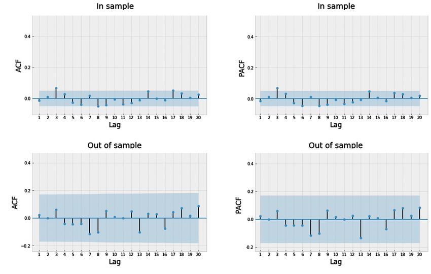
requires stationarity of endogenous feature (Davies in-sample set, the hypothesis of white noise is rejected.
and Newbold, 1979). These issues are examined in this On the other hand, for out-of-the sample period, it is
subsection. not possible to reject the white noise hypothesis.
Initially, the stationarity of the target variable on The autocorrelation and partial correlation plots,
in-sample and out-of-sample sets was inspected using presented in Figure 5, give a deeper insight into lag
Figures 2 and 3. Both plots, especially statistics of significance. For in-sample set, the smallest lags that
rolling mean and variance, suggest that time series is are correlated are the third and the eighth. It justifies
stationary. the need to consider these lags in model specification.
The Augmented Dickey-Fuller test was performed According to out-of-sample chunk, all lags up to
to check stationarity of the time series on in-sample twentieth are not correlated, and it is another result
and out-of-sample data. The algorithm implemented in confirming that the time series during the testing
the Statsmodels package automatically selects number period is a white noise.
of lags to assure that residuals are not autocorrelated.
Table 1 confirms the impression that stock returns are
stationary in both periods. 4.2. Singular models
The Ljung-Box test was performed to verify
whether time series on in-sample and out-of-sample In Table 2, one can see results of all singular models:
chunk is a white noise. Based on the Figure 4 for the SVR, KNN, XGBoost, LightGBM and LSTM,CEEJ • 8(55) • 2021 • pp. 44-62 • ISSN 2543-6821 • DOI: 10.2478/ceej-2021-0004 53 Fig. 3. Nvidia stock returns on out-of-sample set Source: Authors calculations Tab. 1. Results of Augmented Dickey-Fuller test for in-sample set and out-of-sample set Test statistic (in sample) p-value (in sample) Test statistic (out of sample) p-value (out of sample) −11.01
CEEJ • 8(55) • 2021 • pp. 44-62 • ISSN 2543-6821 • DOI: 10.2478/ceej-2021-0004                54

Fig. 4. Results of Ljung-Box test for in-sample set and out-of-sample set. Notes: Figure presents results of Ljung-Box
test of white-noise hypothesis of Nvidia’s stock returns on in-sample set and out-of-sample set
Source: Authors calculations

Fig. 5. ACF and PACF for in-sample and out-of-sample sets. Notes: Figure presents autocorrelation and partial
autocorrelation plots of Nvidia’s stock returns on in-sample and out-of-sample sets
Source: Authors calculations
CEEJ • 8(55) • 2021 • pp. 44-62 • ISSN 2543-6821 • DOI: 10.2478/ceej-2021-0004               55

Tab. 2. Results of singular models on validation and test set (based on stationary variables)

Model (number of attributes)      Set             Hyperparameters                     RMSE        MAE         MedAE

SVR (20)                          Validation      C=0.005206                          0.026924    0.019478    0.014985
                                                  Epsilon=0.087308

SVR (20)                          Test            C=0.005206                          0.036014    0.024916    0.016682
                                                  epsilon=0.087308

KNN (20)                          Validation      Power of Minkowski metric=2         0.026328    0.020331    0.016199
                                                  k=7
                                                  Weight function=uniform

KNN (20)                          Test            Power of Minkowski metric=2         0.039305    0.025935    0.017202
                                                  k=7
                                                  Weight function=uniform

XGBoost (27)                      Validation      Max depth:7                         0.027622    0.020678    0.016553
                                                  Subsample: 0.760762
                                                  Colsample by tree: 0.199892
                                                  Lambda: 0.345263
                                                  Gamma: 0.000233
                                                  Learning rate: 0.2

XGBoost (27)                      Test            Max depth:7                         0.038848    0.027218    0.019782
                                                  Subsample: 0.760762
                                                  Colsample by tree: 0.199892
                                                  Lambda: 0.345263
                                                  Gamma: 0.000233
                                                  Learning rate: 0.2

LGBM (43)                         Validation      Number of leaves:58                 0.025905    0.018803    0.014339
                                                  Min data in leaf:21
                                                  ETA: 0.067318
                                                  Max drop: 52
                                                  L1 regularization: 0.059938
                                                  L2 regularization: 0.050305

LGBM (43)                         Test            Number of leaves:58                 0.038870    0.026283    0.016467
                                                  Min data in leaf:21
                                                  ETA: 0.067318
                                                  Max drop: 52
                                                  L1 regularization: 0.059938
                                                  L2 regularization: 0.050305

LSTM (20)                         Validation      H1                                  0.026565    0.019741    0.014537

LSTM (20)                         Test            H1                                  0.036705    0.024918    0.016772

Notes: Table represents values of 3 metrics of estimation quality: RMSE; MAE; MedAE that SVR, KNN, XGBoost,
LightGBM, LSTM (based on stationary variables) gained on validation and test set, number of attributes and values of
hyperparameters.
H1: number of hidden layers: 1 LSTM layer with dense layer at the end; number of units on each layer: first layer with 20;
number of epochs: 100; activation functions: sigmoid on first layer and linear on dense layer; optimiser function: Adam;
batch size: 32; loss function: MSE.
Source: Author calculations.
CEEJ • 8(55) • 2021 • pp. 44-62 • ISSN 2543-6821 • DOI: 10.2478/ceej-2021-0004 56
Tab. 3. Results of singular models on validation and test set (based on stationary and non-stationary variables)
Model (number of attributes) Set Hyperparameters RMSE MAE MedAE
SVR (27) Validation C=0.005317, epsilon=0.092179 0.025632 0.019126 0.015488
SVR (27) Test C=0.005317, epsilon=0.092179 0.041904 0.025875 0.017279
KNN (40) Validation Power of Minkowski metric=1 0.027021 0.020110 0.013813
k=6
Weight function=uniform
KNN (40) Test Power of Minkowski metric=1 0.039313 0.026863 0.018946
k=6
Weight function=uniform
XGBoost (74) Validation Max depth:3 0.028021 0.021604 0.020396
Subsample: 0.840403
Colsample by tree: 0.605006
Lambda: 4.461698
Gamma: 0.000808
Learning rate: 0.105
XGBoost (74) Test Max depth:3 0.040685 0.026906 0.016939
Subsample: 0.840403
Colsample by tree: 0.605006
Lambda: 4.461698
Gamma: 0.000808
Learning rate: 0.105
LGBM (80) Validation Number of leaves:32 0.025840 0.019361 0.014083
Min data in leaf:38
ETA: 0.099519
Max drop: 51
L1 regularization: 0.060221
L2 regularization: 0.050423
LGBM (80) Test Number of leaves:32 0.037284 0.026295 0.017959
Min data in leaf:38
ETA: 0.099519
Max drop: 51
L1 regularization: 0.060221
L2 regularization: 0.050423
LSTM (20) Validation H2 0.028334 0.021702 0.018201
LSTM (20) Test H2 0.039593 0.028891 0.020576
Notes: Table represents values of 3 metrics of estimation quality: RMSE; MAE; MedAE that SVR, KNN, XGBoost, Light-
GBM, LSTM (based on stationary and non-stationary variables) gained on validation and test set, number of attributes
and values of hyperparameters.
H2: number of hidden layers: 2 LSTM layers with batch normalisation after both of them and dense layer at the end;
number of units on each layer: first layer with 20 units and second with 32 units; number of epochs: 600; activation fun-
ctions: sigmoid on first layer and linear on dense layer; optimiser function: SGD; regularization: bias regularizer at first
layer and activity regularizer (L2) on second LSTM layer; dropout: 0.3 after first LSTM layer; batch size: 16; loss function:
MSE.
Source: Authors calculations.CEEJ • 8(55) • 2021 • pp. 44-62 • ISSN 2543-6821 • DOI: 10.2478/ceej-2021-0004 57
Tab. 4. Performance of ensemble models on test set (models based on stationary variables)
Number of Models (weight) RMSE MAE MedAE
models
2 LightGBM (0.508099), KNN (0.491901) 0.038571 0.025784 0.017147
3 LightGBM (0.342575), KNN (0.331655), LSTM (0.32577) 0.037403 0.025111 0.015704
4 LightGBM (0.260092), KNN (0.251801), LSTM (0.247333), SVR 0.036181 0.024366 0.01599
(0.240775)
5 LightGBM (0.211671), KNN (0.204923), LSTM (0.201287), SVR 0.036106 0.024094 0.015307
(0.19595),
XGBoost (0.18617)
Note: Table represents performance of ensemble models on test set built of models based on stationary variables. Bold
rows respond to the model with the lowest RMSE in that category of ensembling.
Source: Authors calculations.
and LSTM, where usage of non-stationary variables in variables and XGboost (stationary variables). It gains
model estimation resulted in decreased performance. score on RMSE: 0.036746. This result is worse than
performance achieved by ensembling established only
on stationary models.
4.3. Ensemble models To sum up, weights of singular models were
calculated based on its RMSE on validation set. It was
Due to variety of machine learning models in this believed that it will improve forecasts of ensembling
paper, it is very interesting to study the ensembling models. However, surprisingly it is just opposite.
approach. Ensemble models were expected to Singular models perform poorly on test set and
outperform singular models. So, performances of indirectly influence ensembling model’s accuracy (in
ensembling models from three categories mentioned RMSE meaning). Moreover, it has been observed that
in methodology chapter were analysed to confirm the the results converge to the average value (weights
expectations. Table 4 represents results of ensembling are split almost equally) when there is an increase
of models, which are based on stationary variables. in number of models in ensembling algorithm and
As one can see, combining five best singular models thus the variance decreases. Though the models are
LightGBM, KNN, LSTM, SVR, and XGboost provides getting better (RMSE), but in the context of research,
the best score of 0.036106 for RMSE in that category. analysing them loses sense and does not serve any
Results of ensembling models, which are based on purpose.
stationary and non-stationary features, are collected
in the Table 5. Integration of SVR, LightGBM, KNN,
XGBoost and LSTM provides the best results (RMSE: 4.4. Tabular summary
0.038053). Models from Table 4 are better than those
from Table 5 in the mean sense. It is caused by huge To summarise the obtained models and compare its
impact of SVR performance (based on stationary and performances in a systematised way, Tables 7 and 8
non-stationary variables) on validation set in contrast were prepared. Additionally, we used them to examine
to test set, where its prognostic capabilities are weak. two hypotheses. Best ensemble model, which is based
Table 6 aggregates performances of ensemble on stationary variables, is composed of: LightGBM,
models based on all appropriate, available models in KNN, LSTM, SVR and XGBoost. The same models
research repository. The best model connects: SVR are a part of best ensemble model based on stationary
(stationary and non-stationary variables), LightGBM and non-stationary features. Moreover, naive model
(stationary and non-stationary variables), LightGBM results were attached into tables. As one can observe
(stationary variables), KNN (stationary variables), in Table 7, according to Root Mean Squared Error
LSTM (stationary variables), SVR (stationary metric, SVR performed the best on test set among
variables), KNN (stationary and non-stationary models based on stationary variables. LSTM scoreCEEJ • 8(55) • 2021 • pp. 44-62 • ISSN 2543-6821 • DOI: 10.2478/ceej-2021-0004 58
Table 5. Performance of ensemble models on test set (models based on stationary and non-stationary variables)
Number of Models (weight) RMSE MAE MedAE
models
2 SVR (0.504057), LightGBM (0.495943) 0.038730 0.025882 0.017714
3 SVR (0.346773), LightGBM (0.341191), KNN (0.312036) 0.038314 0.026003 0.016682
4 SVR (0.268786), LightGBM (0.264459), KNN (0.241861), 0.038301 0.025793 0.016876
XGBoost (0.224895)
5 SVR (0.220323), LightGBM (0.216777), KNN (0.198253), 0.038053 0.026068 0.016645
XGBoost (0.184346), LSTM (0.180301)
Notes: Table represents performance of ensemble models on test set built of models based on stationary and non-stationary
variables. Bold rows respond to the model with the lowest RMSE in that category of ensembling.
Source: Author calculations.
Tab. 6. Performance of ensemble models on test set (based on all models)
Number of Models (weight) RMSE MAE MedAE
models
2 S+NS SVR (0.504057), S+NS LightGBM (0.495943) 0.03873 0.025882 0.017714
3 S+NS SVR (0.337508), S+NS LightGBM (0.332075), S LightGBM 0.038593 0.025959 0.017321
(0.330417)
4 S+NS SVR (0.255711), S+NS LightGBM (0.251594), S LightGBM 0.038436 0.025665 0.017152
(0.250338), S KNN (0.242357)
5 S+NS SVR (0.206542), S+NS LightGBM (0.203217), S LightGBM 0.037734 0.025267 0.016599
(0.202202), S KNN (0.195756), S LSTM (0.192283)
6 S+NS SVR (0.173976), S+NS LightGBM (0.171176), S LightGBM (0.170321), 0.03681 0.024751 0.01743
S KNN (0.164891), S LSTM (0.161965), S SVR (0.157671)
7 S+NS SVR (0.150427), S+NS LightGBM (0.148006), S LightGBM 0.036871 0.024897 0.016953
(0.147266), S KNN (0.142572), S LSTM (0.140042), S SVR (0.136329), S+NS
KNN (0.135359)
8 S+NS SVR (0.133177), S+NS LightGBM (0.131034), S LightGBM 0.036746 0.024681 0.01647
(0.130379), S KNN (0.126223), S LSTM (0.123983), S SVR (0.120696),
S+NS KNN (0.119837), S XGBoost (0.114672)
9 S+NS SVR (0.119825), S+NS LightGBM (0.117896), S LightGBM (0.117307), 0.036898 0.024757 0.01645
S KNN (0.113568), S LSTM (0.111553), S SVR (0.108595), S+NS KNN
(0.107822), S XGBoost (0.103175), S+NS XGBoost (0.100259)
10 S+NS SVR (0.109125), S+NS LightGBM (0.107368), S LightGBM (0.106832), 0.036899 0.024915 0.016466
S KNN (0.103426), S LSTM (0.101591), S SVR (0.098897), S+NS KNN
(0.098193), S XGBoost (0.093961), S+NS XGBoost (0.091305), S+NS LSTM
(0.089302)
Note: Table represents performance of ensemble models on test set built of all models. Bold rows respond to the model
with the lowest RMSE in that category of ensembling.
Source: Author calculations.CEEJ • 8(55) • 2021 • pp. 44-62 • ISSN 2543-6821 • DOI: 10.2478/ceej-2021-0004 59
Table 7. Performance of models on test set (based on stationary variables)
Metric SVR KNN XGBoost LSTM LGBM Best ensemble Naive model
RMSE 0.036014 0.039305 0.038848 0.036705 0.038870 0.036106 0.050244
MAE 0.024916 0.025935 0.027218 0.024918 0.026283 0.024094 0.034908
MedAE 0.016682 0.017202 0.019780 0.016772 0.016467 0.015307 0.022378
Note: Table represents performance of all models on test set based on stationary variables.
Source: Authors calculations.
Tab. 8. Performance of models on test set (based on stationary and non-stationary variables)
Metric SVR KNN XGBoost LSTM LGBM Best ensemble model Naive model
RMSE 0.041904 0.039313 0.040685 0.039593 0.037284 0.038053 0.050244
MAE 0.025875 0.026863 0.026906 0.028891 0.026295 0.026068 0.034908
MedAE 0.017279 0.018946 0.016939 0.020576 0.017959 0.016645 0.022378
Note: Table represents performance of all models on test set based on stationary and non-stationary variables.
Source: Authors calculations.
is also satisfactory for the aim of the research. In on stationary features) outperformed other models
this case, ensemble model cannot overpass singular based on Table 9. Figure 6 presents its results on
models, particularly SVR. All the established models the test set. This plot suggests that, during the first
(from Table 7) were able to surpass naïve model. period of testing (before a bear market), model has a
As presented in Table 8, LightGBM gained the low and almost constant variance, however during
best results on the test set. Other models performed second period fitted values deviates significantly,
noticeably worse on RMSE metric. Interestingly but model can detect arising spikes. Comparing
SVR, which has the highest RMSE, gained the lowest three types of ensemble models, the one based on the
Mean Absolute Error. It is due to the fact that RMSE stationary approach returns the best forecasts. The
is sensitive to outliers. Ensemble approach fails to third ensemble model, which is based on all available
introduce an improvement in prediction. As before, singular models, does not gain additional impact on
naive model has the worst outcome on test set. this study.
For further deeper insight into models efficiency,
best ensemble models from 3 categories were compared 5. Conclusions
in Table 9 with singular models that perform the best
against stationary variables and all variables. Naive Note that that all hypotheses mentioned have been
model was also included as a benchmark. Among analysed and answered in this research. The main
models based on stationary features, SVR occurred purpose of this study was to effectively forecast the
to surpass other models. RMSE obtained by Support daily stock returns of Nvidia Corporation company
Vector Regression was 0.036014. In the group of quoted on the Nasdaq Stock Market, using numerous
models built from stationary and non-stationary exogenous explanatory variables. Considering
variables, LightGBM was the best one with score of these variables, the major hypothesis that has been
RMSE at level equal to 0.037284. Therefore, models verified in this paper is that it is possible to construct
based on stationary features give higher precision prediction model of Nvidia daily return ratios, which
of forecast than models estimated on stationary and can outperform both simple naive and econometric
non-stationary variables. All in all, SVR model (based models. According to results, outperforming simpleCEEJ • 8(55) • 2021 • pp. 44-62 • ISSN 2543-6821 • DOI: 10.2478/ceej-2021-0004 60
Tab. 9. Performance of best models on test set (ensemble and primary models)
Metric Best stationary Best stationary Best ensemble Best station- Best stationary Naive
ensemble model + non-stationary model based on ary model + non-stationary model
ensemble model all models – SVR model –
LGBM
RMSE 0.036106 0.038053 0.036746 0.036014 0.037284 0.050244
MAE 0.024094 0.026068 0.024681 0.024916 0.026295 0.034908
MedAE 0.015307 0.016645 0.01647 0.016682 0.017959 0.022378
Note: Table represents compof performances of best singular and ensemble models from each category and naive model
on test set.
Source: Authors calculations.
Fig. 6. Performance on test set of the best model in research – SVR (based on stationary variables)
Source: Authors calculations
naive model is not a challenging task because every final vs one-month-ahead approach). Prepared models
model had much lower RMSE of forecast residuals. It were not able to cope with market fluctuations that
is found that econometric models such as ARIMA and began in October 2018. It comes from specificity of
ARIMAX are not able to rationally forecast during testing set, where variance increased drastically on
the white noise period (they converge to 0). Thus an unprecedented scale. Models based on stationary
machine learning models are more appropriate than variables perform better than models based on
traditional statistical-econometric methods in case of stationary and non-stationary variables (RMSE: SVR
stock returns prediction. The best score was obtained with 0.036014 vs LightGBM with 0.037284). It is
by SVR based on stationary variables, whereas Abe consistent with results obtained by Yang and Shahabi
and Nakayama (2018) show that DNN has much (2005) in classification problem, in which correlation
better prognostic properties than SVR. The reason among features is essential. Adebiyi, Adewumi and
for that might be forecasting window (one-day-ahead Ayo (2014) have shown the superiority of neuralCEEJ • 8(55) • 2021 • pp. 44-62 • ISSN 2543-6821 • DOI: 10.2478/ceej-2021-0004 61
networks model over ARIMA model in prediction Adebiyi, A. A., Adewumi, A. O., & Ayo, C. K. (2014).
of profits from shares. Surprisingly ranking-based Comparison of ARIMA and artificial neural networks
ensemble models did not perform better than singular models for stock price prediction. Journal of Applied
ones, which is contrary to conclusions drawn by Mathematics 2014. https://doi.org/10.1155/2014/614342
Adhikari et al. (2015). Categories of variables which Adhikari, R., Verma, G., & Khandelwal, I. (2015).
are suggested in literature are significant in final A model ranking based selective ensemble approach
models. The combination of technical analysis and for time series forecasting. Procedia Computer Science,
fundamental analysis, as proposed by Beyaz et al. 48, 14–21. https://doi.org/10.1016/j.procs.2015.04.104
(2018), turned out to be a good idea. Features selection
algorithms extracted many features based on Google Ahmed, F., Asif, R., Hina, S., & Muzammil, M.
Trends entries and this fact is consistent with the (2017). Financial market prediction using Google
discovery of Ahmed et al. (2017). It is worth noticing Trends. International Journal of Advanced Computer
that singular variables recommended by literature e.g. Science and Applications, 8(7), 388–391. https://doi.
Mahmoud and Sakr (2012) were always rejected in org/10.14569/IJACSA.2017.080752
feature extraction. Altman, N. S. (1992). An introduction to kernel
We state that our contribution to literature is and nearest-neighbor nonparametric regression.
twofold. First, we provide added value to the strand The American Statistician, 46(3), 175–185. https://doi.
of literature on the choice of model class to the org/10.2307/2685209
stock returns prediction problem. Second, our study Beyaz, E., Tekiner, F., Zeng, X. J., & Keane, J.
contributes to the thread of selecting exogenous (2018). Stock Price Forecasting Incorporating Market
variables and the need for their stationarity in the case State. 2018 IEEE 20th International Conference on
of time series models. High Performance Computing and Communications.
There exist many noticeable challenges on this field https://doi.org/10.1109/HPCC/SmartCity/
that should be investigated in the future. Simple naive DSS.2018.00263
model performed poorly on test set. Hence, other models Bontempi, G., Taieb, S., & Borgne, Y. A.
should be considered as a benchmark. Furthermore, this (2012). Machine learning strategies for time series
model should not have a variance converging to zero, forecasting. In European business intelligence summer
which is an important problem. Due to the specifics school (pp. 62–77). Berlin, Germany: Springer. https://
of the stock exchange, models degrade very quickly. doi.org/10.1007/978-3-642-36318-4_3
Perhaps a reasonable approach would be to build and
Box, G., & Jenkins, G. (1970). Time Series Analysis:
calibrate models (based on new variables) in a quarterly
Forecasting and Control. San Francisco, CA: Holden-
period. Additionally, Nested Cross Validation algorithm
Day.
might be applied. As ARIMAX failed, GARCH model
could be examined alternately. Another improvement Chen, T., & Guestrin, C. (2016). Xgboost: A
could be obtained using different algorithms of scalable tree boosting system. In Proceedings of the 22nd
ensembling (blending and stacking). As the part of study ACM SIGKDD International Conference on Knowledge
is connected with variables, sentimental analysis should Discovery and Data Mining (pp. 785–794). https://doi.
be taken into account. org/10.1145/2939672.2939785
Chen, K., Zhou, Y., & Dai, F. (2015). A LSTM-
based method for stock returns prediction: A case
References study of China stock market. In 2015 IEEE International
Abazovic, F. (2018). Nvidia stock dropped for the Conference on Big Data (Big Data). https://doi.
wrong reason. Retrieved from https://www.fudzilla. org/10.1109/bigdata.2015.7364089
com/news/ai/47637-nvidia-stock-dropped-for-the- Chou, J. S., & Tran, D. S. (2018). Forecasting energy
wrong-reason consumption time series using machine learning
Abe, M., & Nakayama, H. (2018). Deep learning techniques based on usage patterns of residential
for forecasting stock returns in the cross-section. householders. Energy, 165, 709–726. https://doi.
org/10.1016/j.energy.2018.09.144
Pacific-Asia Conference on Knowledge Discovery and
Data Mining. 273–284. https://doi.org/10.1007/978-3- Vapnik, V., Drucker, H., Burges, C. J., Kaufman,
319-93034-3_22 L., & Smola, A. (1997). Support vector regressionCEEJ • 8(55) • 2021 • pp. 44-62 • ISSN 2543-6821 • DOI: 10.2478/ceej-2021-0004 62
machines. Advances in Neural Information Processing on the panel data analysis; evidence from Karachi
Systems, 9, 155–161. Stock exchange (KSE). Research Journal of Finance and
Accounting, 9(3), 84–96.
Eassa, A. (2018). Why NVIDIA’s Stock Crashed.
Retrieved from https://finance.yahoo.com/news/ Nvidia Corporation. (2018). Nvidia Corporation
why-nvidia-apos-stock-crashed-122400380.html Annual Review. Retrieved from https://s22.q4cdn.
com/364334381/files/doc_financials/annual/2018/
Emir, S., Dincer, H., & Timor, M. (2012). A stock
NVIDIA2018_AnnualReview-(new).pdf.
selection model based on fundamental and technical
analysis variables by using artificial neural networks Pai, P. F., & Lin, C. S. (2005). A hybrid ARIMA
and support vector machines. Review of Economics & and support vector machines model in stock
Finance, 2(3), 106–122. price forecasting. Omega, 33, 497–505. https://doi.
org/10.1016/j.omega.2004.07.024
Hatta, A. J. (2012). The company fundamental
factors and systematic risk in increasing stock price. Preis, T., Moat, H. S., & Stanley, E. H. (2013).
Journal of Economics, Business and Accountancy, 15(2), Quantifying trading behavior in financial markets
245–256. http://doi.org/10.14414/jebav.v15i2.78 using Google Trends. Scientific Reports, 3(1684), 1–6.
https://doi.org/10.1038/srep01684
Hill, J. B., & Motegi, K. (2019). Testing the
white noise hypothesis of stock returns. Economic Rather, A. M., Agarwal, A., & Sastry, V. N.
Modelling, 76, 231–242. https://doi.org/10.1016/j. (2015). Recurrent neural network and a hybrid
econmod.2018.08.003 model for prediction of stock returns. Expert Systems
with Applications, 42(6), 3234–3241. https://doi.
Hochreiter, S., & Schmidhuber, J. (1997). Long
org/10.1016/j.eswa.2014.12.003
short-term memory. Neural Computation, 9(8), 1735–
1780. https://doi.org/10.1162/neco.1997.9.8.1735 Shim, J. K., & Siegel, J. G. (2007). Handbook of
Financial Analysis, Forecasting, and Modeling (p. 255).
Ke, G., Meng, Q., Finley, T., Wang, T., & Chen, W.
Chicago, USA: CCH.
(2017). Lightgbm: A highly efficient gradient boosting
decision tree. Advances in Neural Information Processing Stanković, J., Marković, J., & Stojanović, M. (2015).
Systems, 30, 3146–3154. Investment strategy optimization using technical
analysis and predictive modeling in emerging markets.
Kozachenko, L. F., & Leonenko, N. N. (1987).
Procedia Economics and Finance, 19, 51–62. https://doi.
Sample estimate of the entropy of a random vector.
org/10.1016/S2212-5671(15)00007-6
Problemy Peredachi Informatsii, 23(2), 9–16.
Whittle, P. (1951). Hypothesis Testing in Time Series
Laptev, N., Yosinski, J., Li, L. E., & Smyl, S. (2017).
Analysis. Uppsala, Sweden: Almqvist & Wiksells boktr.
Time-series extreme event forecasting with neural
networks at Uber. International Conference on Machine Yang, K., & Shahabi, C. (2005). On the stationarity
Learning, 34, 1–5. of multivariate time series for correlation-based data
analysis. In Proceedings of the Fifth IEEE International
Lo, A. W. (2004). The adaptive markets hypothesis:
Conference on Data Mining, Houston. https://doi.
Market efficiency from an evolutionary perspective.
org/10.1109/ICDM.2005.109
The Journal of Portfolio Management, 30(5), 15–29.
https://doi.org/10.3905/jpm.2004.442611 Zeytinoglu, E., Akarim, Y. D., & Celik, S. (2012).
The impact of market-based ratios on stock returns:
Mahmoud, A., & Sakr, S. (2012). The predictive
The evidence from insurance sector in Turkey.
power of fundamental analysis in terms of stock return
International Research Journal of Finance and Economics,
and future profitability performance in Egyptian
84, 41–48.
Stock Market: Empirical Study. International Research
Journal of Finance & Economics, 92(1), 43–58. Zheng, A., & Jin, J. (2017). Using AI to make
predictions on stock MARKET. Stanford University.
Milosevic, N. (2016). Equity forecast: Predicting
Retrieved from http://cs229.stanford.edu/proj2017/
long term stock price movement using machine
final-reports/5212256.pdf
learning. Journal of Economics Library, 3(2), 288–294.
http://doi.org/10.1453/jel.v3i2.750
Muhammad, S., & Ali, G. (2018). The relationship
between fundamental analysis and stock returns basedYou can also read