Testing the ability of species distribution models to infer variable importance
←
→
Page content transcription
If your browser does not render page correctly, please read the page content below
Zurich Open Repository and
                                                                         Archive
                                                                         University of Zurich
                                                                         Main Library
                                                                         Strickhofstrasse 39
                                                                         CH-8057 Zurich
                                                                         www.zora.uzh.ch

 Year: 2020

Testing the ability of species distribution models to infer variable importance

                                    Smith, Adam B ; Santos, Maria J

Abstract: Models of species’ distributions and niches are frequently used to infer the importance of
range‐ and niche‐defining variables. However, the degree to which these models can reliably identify
important variables and quantify their influence remains unknown. Here we use a series of simulations to
explore how well models can 1) discriminate between variables with different influence and 2) calibrate the
magnitude of influence relative to an ‘omniscient’ model. To quantify variable importance, we trained
generalized additive models (GAMs), Maxent and boosted regression trees (BRTs) on simulated data
and tested their sensitivity to permutations in each predictor. Importance was inferred by calculating
the correlation between permuted and unpermuted predictions, and by comparing predictive accuracy of
permuted and unpermuted predictions using AUC and the continuous Boyce index. In scenarios with
one influential and one uninfluential variable, models failed to discriminate reliably between variables
when training occurrences were < 8–64, prevalence was > 0.5, spatial extent was small, environmental
data had coarse resolution and spatial autocorrelation was low, or when pairwise correlation between
environmental variables was |r| > 0.7. When two variables influenced the distribution equally, impor-
tance was underestimated when species had narrow or intermediate niche breadth. Interactions between
variables in how they shaped the niche did not affect inferences about their importance. When variables
acted unequally, the effect of the stronger variable was overestimated. GAMs and Maxent discriminated
between variables more reliably than BRTs, but no algorithm was consistently well‐calibrated vis‐à‐vis
the omniscient model. Algorithm‐specific measures of importance like Maxent’s change‐in‐gain metric
were less robust than the permutation test. Overall, high predictive accuracy did not connote robust
inferential capacity. As a result, requirements for reliably measuring variable importance are likely more
stringent than for creating models with high predictive accuracy.

DOI: https://doi.org/10.1111/ecog.05317

Posted at the Zurich Open Repository and Archive, University of Zurich
ZORA URL: https://doi.org/10.5167/uzh-193377
Journal Article
Published Version

The following work is licensed under a Creative Commons: Attribution 3.0 Unported (CC BY 3.0)
License.

Originally published at:
Smith, Adam B; Santos, Maria J (2020). Testing the ability of species distribution models to infer variable
importance. Ecography, 43(12):1801-1813.
DOI: https://doi.org/10.1111/ecog.05317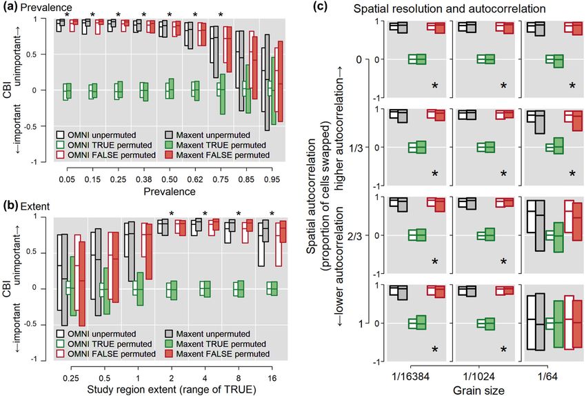
ECOGRAPHY
Research
Testing the ability of species distribution models to infer
variable importance

Adam B. Smith and Maria J. Santos

A. B. Smith (https://orcid.org/0000-0002-6420-1659) ✉ (adam.smith@mobot.org), Center for Conservation and Sustainable Development, Missouri
Botanical Garden, Saint Louis, MO, USA. – M. J. Santos, Univ. Research Priority Program in Global Change and Biodiversity and Dept of Geography,
Univ. of Zürich, Zürich, Switzerland.

Ecography                                     Models of species’ distributions and niches are frequently used to infer the importance
43: 1801–1813, 2020                           of range- and niche-defining variables. However, the degree to which these models can
doi: 10.1111/ecog.05317                       reliably identify important variables and quantify their influence remains unknown.
                                              Here we use a series of simulations to explore how well models can 1) discriminate
Subject Editor: Cory Merow                    between variables with different influence and 2) calibrate the magnitude of influence
Editor-in-Chief: Miguel Araújo                relative to an ‘omniscient’ model. To quantify variable importance, we trained general-
Accepted 24 July 2020                         ized additive models (GAMs), Maxent and boosted regression trees (BRTs) on simu-
                                              lated data and tested their sensitivity to permutations in each predictor. Importance
                                              was inferred by calculating the correlation between permuted and unpermuted predic-
                                              tions, and by comparing predictive accuracy of permuted and unpermuted predictions
                                              using AUC and the continuous Boyce index. In scenarios with one influential and one
                                              uninfluential variable, models failed to discriminate reliably between variables when
                                              training occurrences were < 8–64, prevalence was > 0.5, spatial extent was small,
                                              environmental data had coarse resolution and spatial autocorrelation was low, or when
                                              pairwise correlation between environmental variables was |r| > 0.7. When two vari-
                                              ables influenced the distribution equally, importance was underestimated when spe-
                                              cies had narrow or intermediate niche breadth. Interactions between variables in how
                                              they shaped the niche did not affect inferences about their importance. When vari-
                                              ables acted unequally, the effect of the stronger variable was overestimated. GAMs and
                                              Maxent discriminated between variables more reliably than BRTs, but no algorithm
                                              was consistently well-calibrated vis-à-vis the omniscient model. Algorithm-specific
                                              measures of importance like Maxent’s change-in-gain metric were less robust than the
                                              permutation test. Overall, high predictive accuracy did not connote robust inferential
                                              capacity. As a result, requirements for reliably measuring variable importance are likely
                                              more stringent than for creating models with high predictive accuracy.

                                              Keywords: ecological niche model, sample size, spatial scale species distribution
                                              model, statistical inference, variable importance

                                              ––––––––––––––––––––––––––––––––––––––––
                                              © 2020 The Authors. Ecography published by John Wiley & Sons Ltd on behalf of Nordic Society Oikos
www.ecography.org                             This is an open access article under the terms of the Creative Commons
                                              Attribution License, which permits use, distribution and reproduction in any
                                              medium, provided the original work is properly cited.                                        1801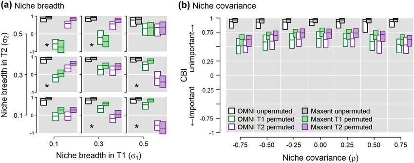
Introduction                                                      and Bühlmann 2010). To measure sensitivity of the model to
                                                                  changes in the variable, we use the permute-after-calibration
What environmental factors determine species’ ranges and          test (Breiman 2001) which compares unpermuted and per-
environmental tolerances? The answer to this question             muted predictions. To compare unpermuted and permuted
remains elusive for most species on Earth despite being cru-      predictions, we calculated for each the continuous Boyce
cial for addressing long-standing issues in theoretical and       index (CBI) and the area under the receiver–operator curve
applied ecology. Although manipulative field- and labora-         (AUC). CBI indicates how well predictions serve as an index
tory-based studies can identify factors that shape niches and     of the probability of presence (Boyce et al. 2002, Hirzel et al.
ranges (Hargreaves et al. 2014, Lee-Yaw et al. 2016), for         2006), while AUC indicates how well predictions differen-
most species logistical difficulties preclude examining large     tiate between presence and non-presence sites. We also cal-
numbers of variables and studying range limits across broad       culated the correlation between unpermuted and permuted
geographic scales. Alternatively, environmental limits can        predictions (COR; Breiman 2001), which reflects differences
be inferred using models of species’ geographic ranges and        between the two sets of predictions. Permuting an important
niches. These ecological niche models and species distribu-       variable in a model should decrease CBI, AUC and COR.
tion models (SDMs) are constructed by correlating observa-            To simulate species’ distributions, we defined a generative
tions of occurrence with data on environmental conditions         function of one or two variables on the landscape, then used
at occupied sites. Indeed, one of the most common uses for        it to produce a raster of the probability of occurrence. For
SDMs is to identify important variables (e.g. 227 inferential     each cell, true occupancy was determined using a Bernoulli
studies analyzed by Bradie and Leung 2017 using the Maxent        draw with the probability of success equal to the simulated
algorithm alone). However, we are aware of no studies that        probability of presence (Meynard and Kaplan 2013). We
systematically evaluate how well SDMs measure variable            then calibrated and evaluated three SDM algorithms: gen-
importance. Compared to the attention devoted to under-           eralized additive models (GAMs; Wood 2006), Maxent
standing predictive accuracy of models of niches and distri-      (Phillips et al. 2006) and boosted regression trees (BRTs;
butions (Elith et al. 2006, Smith et al. 2013, Buklin et al.      Elith et al. 2008). Full details of model calibration are pre-
2015, Guevara et al. 2018, Norberg et al. 2019), the lack of      sented in Supplementary material Appendix 1. Briefly, (unless
research on the efficacy of these same models for identifying     otherwise stated) SDMs were calibrated using 200 occur-
important variables is a striking oversight.                      rences and 10 000 (Maxent and GAMs) or 200 (BRTs) back-
   The ability of an SDM to infer variable importance will        ground sites (Barbet-Massin et al. 2012). Predictive accuracy
likely be affected by factors that are intrinsic to the species   and inferential capacity were evaluated using 200 distinct
(e.g. niche breadth) and by factors that are extrinsic to the     test occurrences plus either 10 000 background sites (CBI,
species and thus at least nominally under control of the          AUCbg and CORbg) or 200 absences (AUCpa and CORpa;
modeler (e.g. sample size, study region extent, etc.). Here       Meynard et al. 2019). In addition to the permute-after-cal-
we utilize a reductionist approach based on virtual species       ibration test, for each of the experiments we also evaluated
(Meynard et al. 2019) to systematically evaluate a set of         algorithm-specific measures of variable importance: AIC-
intrinsic and extrinsic factors expected to influence variable    based variable weighting for GAMs (Burnham and Anderson
inference. Our goal was to identify the minimal conditions        2002); contribution, permutation and change-in-gain tests
under which each factor allows robust inference of variable       for Maxent (Phillips and Dudík 2008); and deviance reduc-
importance, assuming all other conditions are optimal. We         tion for BRTs (Elith et al. 2008). To streamline discussion,
conducted nine simulation experiments to explore circum-          we present results only for Maxent and CBI in the main text
stances that affect inference. We start with the simplest case    (Supplementary material Appendix 3–9 present the complete
in which a species’ range is determined by a single ‘TRUE’        set of results).
variable, but the SDMs are presented with data on this vari-          In our simulations there is no process-based spatial auto-
able plus an uncorrelated ‘FALSE’ variable with no effect         correlation in species occurrences arising from dispersal,
on distribution. We then explore the effects of sample size,      disturbance or similar processes. As a result, occurrences at
spatial scale and collinearity between variables. Finally, we     sites are statistically independent of one another regardless
examine cases where the species’ distribution is shaped by        of their proximity, which obviates the need to use geographi-
two collinear TRUE variables that can be correlated and can       cally distinct training and test sites. This is a convenience that
interact to define the niche.                                     is unlikely to be met in real-world situations where robust
                                                                  inference requires test data that is geographically and/or
Methods                                                           temporally as independent as possible from training data
                                                                  (Roberts et al. 2017, Fourcade et al. 2018).
General approach                                                      For each level of a factor we manipulated in an experiment
                                                                  (e.g. landscape size), we generated 100 landscapes with train-
We assume a variable is ‘important’ in a model if the model       ing and test data sets, then calibrated and evaluated GAM,
has high predictive accuracy and if predictions are highly        Maxent and BRT models on each set. As a benchmark, we
sensitive to changes in values of that variable (Meinshausen      used an ‘omniscient’ (OMNI) model which was exactly the

1802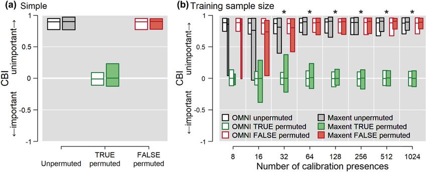
same as the generative model used to create the species’ prob-       Experiment 2: training sample size
ability of occurrence (Meynard et al. 2019). We evaluated the
OMNI model with the same set of test data used to evalu-             Next, we examined how the number of occurrences used in
ate the SDMs. To generate predictions from permuted vari-            the training sample affects estimates of variable importance.
ables, for a given level of a factor, data iteration and SDM         We used the same landscape and probability of occurrence
algorithm, we created 30 permutations of each variable, cal-         as in Experiment 1. The number of training occurrences was
culated test statistics (CBI, AUC and COR) for each, then            varied across the doubling series 8, 16, 32, …, 1024, but the
took the average test statistic value across these 30 sets. Since    number of test sites was kept the same (200 occurrences and
OMNI does not use training data, variation in test statistics is     either 10 000 background sites or 200 absences).
due solely to stochastic differences in test sites and permuta-
tions between iterations.                                            Experiment 3: prevalence
    We know a priori that levels of a factor are different, so our
                                                                     We then explored the effects of prevalence (mean probabil-
interest is in the effect size of each factor level (White et al.
                                                                     ity of occurrence). The species responded to TRUE as per a
2014), which can be discerned by eye. For a given test sta-
                                                                     logistic function,
tistic (CBI, AUC or COR), we assessed the capacity of the
permute-after-calibration test to assess discrimination (quali-
tative differences between variables with different influence)                        exp ( b1 ´ ( TRUE - b2 ))
and calibration (how well the distribution of the SDM’s test         Pr ( occ ) =                                                (2)
                                                                                    1 + exp ( b1 ´ ( TRUE - b2 ) )
statistic matches that of the test statistic generated using the
unbiased OMNI model). We designated a test as having
‘reliable discrimination’ if there is complete lack of overlap       where non-zero values of the offset parameter β2 shift the
between the inner 95% of the distribution of the test statistic      range across the landscape, thereby altering prevalence
between the permuted and unpermuted predictions across               (Supplementary material Appendix 2 Fig. A2). This allows
the 100 iterations. We designated a test as having ‘reliable         us to manipulate prevalence while not changing study region
calibration’ by comparing the distribution of the test statis-       extent, which is almost impossible in real-world situations.
tic between the SDM and OMNI: the range of the SDM’s                 We set β1 equal to 2 and chose values of β2 that varied preva-
inner 95% of values across data iterations are within ±10%           lence in 9 steps from 0.05 to 0.95.
of OMNI’s range, and the SDM’s median value is within the
40th and 60th percentile of OMNI’s median value. Under
this definition, neither CBI, CORpa, nor CORbg were ever             Experiment 4: study region extent
well-calibrated, although in a few cases AUCpa and AUCbg
yielded well-calibrated outcomes (Supplementary material             In real-world situations enlarging a study region typically
Appendix 5–6). Hence, hereafter we focus on discrimination           decreases prevalence (Anderson and Raza 2010) while also
accuracy.                                                            increasing the range of variability in environmental variables
                                                                     (VanDerWal et al. 2009). In this experiment we isolate the
Experiment 1: simple scenario                                        effect of increasing the extent of the study region on the range
                                                                     of environmental variation in the TRUE variable. Landscape
In the simplest scenario we assumed the species’ probability         size was varied along the doubling series 128, 256, 512, …,
of occurrence is determined by a logistic generative function        8192 cells on a side, each matched with an increasing range
of a single TRUE variable:                                           of the TRUE variable from (−0.125, 0.125) for the smallest
                                                                     landscape to (−8, 8) for the largest (Supplementary material
                                                                     Appendix 2 Fig. A3). FALSE was spatially randomly distrib-
                exp (b ´ TRUE )
Pr ( occ ) =                                                  (1)    uted and had the range (−1, 1). The species responded to
               1 + exp (b ´ TRUE )                                   TRUE as per a logistic function (Eq. 1). As a result, increas-
                                                                     ing extent did not change prevalence.
where β represents the strength of the response. We set β = 2
which produced a moderate gradient in the probability of             Experiment 5: spatial resolution and autocorrelation
presence across the landscape. The TRUE variable has a linear        of environmental data
gradient in geographic space ranging from −1 to 1 across a
square landscape 1024 cells on a side (Supplementary mate-           In this experiment we explored the effects of spatial autocor-
rial Appendix 2 Fig. A1). As a result, the species’ probability      relation and spatial resolution (grain size) of environmental
of occurrence is symmetrically distributed with an inflection        data on estimates of variable importance. We began with a
point midway across the landscape. For each of the 100 data          linear TRUE and random FALSE variable distributed across
iterations, SDMs were trained using values of TRUE plus              a landscape with 1024 cells on a side. When unperturbed,
values of a spatially random FALSE variable with the range           the linear gradient of the TRUE variable has a high degree
(−1, 1). The FALSE variable represents a variable ‘mistakenly’       of spatial autocorrelation because cells close to one another
assumed to influence the species’ distribution.                      have similar values. To manipulate spatial autocorrelation,

                                                                                                                                1803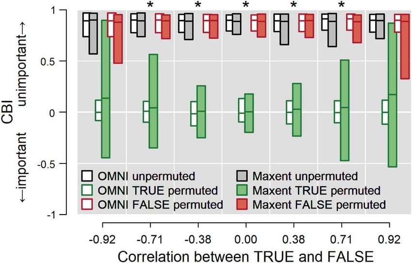
we randomly swapped values of a set proportion of cell val- 1
ues (no cells, or one third, two thirds, or all of the cells). Pr (occ ) =
Swapping values reduces spatial autocorrelation in the TRUE 2ps1s2 1 − r 2
variable because cells with dissimilar values are more likely to (3)
T 12 T 1 ×T 2 T 22
be close to one another (Supplementary material Appendix 2 exp − 2 + −
( ) ( ) ( )
r
Fig. A4). FALSE had a level of spatial autocorrelation no dif- 2s1 1 − r 2 s1s2 1 − r 2 2s22 1 − r 2
ferent from random, regardless of swapping.
We assumed the species responded to the environment at
the ‘native’ 1/1024th scale of the landscape. Probability of Niche breadth in T1 and T2 is determined by σ1 and σ2.
occupancy was modeled with Eq. 1, and training and test Importantly, decreasing σi increases the degree to which a
sites were sampled at this ‘native’ resolution. In some of the variable restricts distribution, meaning that σi and variable
simulations we changed the spatial resolution of the envi- importance are inversely related. Parameter ρ determines the
ronmental data presented to the SDMs by resampling the degree of ‘niche covariance,’ or interaction between variables
environmental rasters to a finer resolution with 16 384 cells in shaping the niche.
or to a coarser resolution with 64 cells on a side using bilin- In Experiment 7 we examined the effects of niche breadth
ear interpolation (sample size was kept the same regardless of by varying σ1 and σ2 across all combinations of 0.1, 0.3 and
resolution). In summary, we created a landscape, (possibly) 0.5. We set niche covariance ρ = 0 and kept T1 and T2 uncor-
swapped cells, modeled the species’ distribution and located related on the landscape. In Experiment 8 we investigated the
training and test sites at the ‘native’ scale, then assigned envi- effects of niche covariance by varying ρ from −0.75 to 0 to
ronmental values to sites based on the landscape at the (pos- 0.75. We used intermediate niche breadth (σ1 and σ2 = 0.3)
sibly) resampled resolution. This recreates a realistic situation and kept T1 and T2 uncorrelated on the landscape. Finally, in
where occurrences represent the scale of the true response but Experiment 9 we explored all combinations of niche breadth
environmental data used to predict the response are available (varying σ1 and σ2 across 0.1, 0.3, and 0.5), niche covari-
at a (potentially) different resolution. We explored all com- ance (varying ρ across −0.5, 0, and 0.5) and collinearity
binations of grain size (cell size of 1/16 384th, 1/1024th and between T1 and T2 on the landscape (varying r across −0.71,
1/64th of the landscape’s linear dimension) and spatial auto- 0, and 0.71).
correlation (swapping no cells, or one third, two thirds or all
of the cells; Supplementary material Appendix 2 Fig. A4). Reproducibility
Experiment 6: collinearity between environmental We created the R (R Core Team) package ‘enmSdmPre-
variables dImport’ (Smith 2019) for generating virtual species and
assessing variable importance. Code for the experiments
Next, we explored the effects collinearity (correlation) and figures in this article is available at . The pack-
had a logistic response (Eq. 1) to TRUE, which has a linear age and code for the experiments depend primarily on the
gradient across the landscape. In contrast to previous experi- ‘dismo’ (Hijmans et al. 2017), ‘raster’ (Hijmans 2019) and
ments, FALSE also has a linear trend which is rotated relative ‘enmSdm’ (Smith 2020) packages for R.
to the gradient in TRUE to alter the correlation between the
variables. We used a circular landscape to ensure no change
in the univariate frequencies of the variables with rotation. Results
The two variables are uncorrelated when their relative rota-
tion is 90°, and positive or negative if less than or more than In each experiment we assessed six metrics (Box 1). Results
90°, respectively (Supplementary material Appendix 2 Fig. from OMNI serve as a benchmark for the SDM because
A5). We used rotations of FALSE relative to TRUE from they represent the best an SDM could be expected to do
22.5 to 157.5° in steps of 22.5°, which produced correlations given only variation in test data. Thus, when unpermuted
between the two variables ranging from r = −0.91 to 0.91. predictions from OMNI have poor predictive accuracy, or
Both variables had values in the range (−1, 1). when OMNI with permuted predictions fails to discriminate
between variables, the SDM should also fail. Importantly,
Experiments 7, 8 and 9: two influential variables results for a given level of a manipulation represent out-
comes across multiple data iterations, each of which typi-
In the final experiments the species’ niche was shaped by two cally spanned a much smaller range (during permutation)
influential variables, T1 and T2, which both have linear gra- than the full set of models. Modelers typically have just one
dients on a circular landscape and values in the range (−1, set of data for a species, so variation for a single data instance
1). The species responds to both T1 and T2 as per a Gaussian will underestimate the uncertainty inherent in the data sam-
bivariate function: pling process.
1804
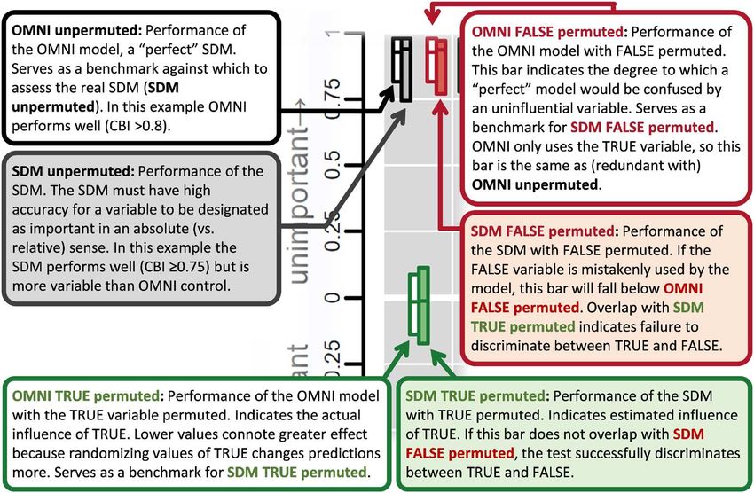
Box 1 Interpreting the permute-after-calibration test of variable importance
  Bars represent the inner 95% of values of CBI across 100 data iterations. Horizontal lines within each bar represent median CBI across
  the 100 data iterations.

Experiment 1: simple scenario                                          and unpermuted CBI was greater at high prevalence than in
                                                                       OMNI (Fig. 2a).
OMNI with unpermuted variables had high predictive accu-
racy (Fig. 1a). OMNI TRUE and FALSE permuted did not
overlap, meaning that the variables could be successfully dif-         Experiment 4: study region extent
ferentiated. Maxent performed similarly, although with more            Increasing landscape extent (the range of the TRUE variable)
variation around TRUE permuted compared to OMNI                        caused predictive accuracy of OMNI unpermuted to peak at
TRUE permuted.                                                         intermediate extents where the range of TRUE was from 2 to 4
                                                                       (i.e. landscapes of 1024–2048 cells on a side; Fig. 2b). OMNI
Experiment 2: training sample size                                     failed to reliably discriminate between TRUE and FALSE on
OMNI does not use training data, so always correctly dis-              the smallest landscapes (range of TRUE ≤ 0.5). Maxent was
criminated TRUE from FALSE regardless of training sample               less robust to small extents, failing when the range of TRUE
size (Fig. 1b). Maxent performed as well as OMNI unper-                was ≤ 1 (Fig. 2b). The worsening performance of OMNI
muted when sample size was ≥ 64, but below this Maxent                 unpermuted at large extents might be due to the sensitivity
had much greater variability than OMNI and was unable                  of CBI to test presences that are located in areas with a very
to reliably discriminate between TRUE and FALSE at n <                 low probability of presence and to potential underfitting of
32. At the smallest sample size (n = 8), Maxent often yielded          Maxent (Supplementary material Appendix 10).
intercept-only models that could not be used to calculate
CBI, which requires variation in predictions for calculation.          Experiment 5: spatial resolution and autocorrelation
                                                                       of environmental data
Experiment 3: prevalence
                                                                       In this experiment, the ‘true’ importance of TRUE and
Increasing prevalence (mean probability of occurrence)                 FALSE is indicated by OMNI at the ‘native’ resolution of
reduced unpermuted OMNI’s predictive accuracy and                      1/1024 (middle column of subpanels in Fig. 2c). Results for
increased variability. As a result, OMNI often performed no            OMNI at the other resolutions represent the outcome that
better than random when prevalence was ≥ 0.85 (Fig. 2a) and            would be obtained if a modeler had perfect knowledge of
could not discriminate between TRUE and FALSE. Maxent                  the species’ response to the environment but only had envi-
was qualitatively the same, although variation in permuted             ronmental data available at finer or coarser resolutions than

                                                                                                                                     1805
Figure 1. (a) Experiment 1: simple scenario. The species’ range is influenced solely by a TRUE variable, but data on an uninfluential FALSE
variable is also ‘mistakenly’ presented to models. Maxent successfully discriminates between the two variables (no overlap between green and
red bars). See Box 1 for further interpretation. (b) Experiment 2: sample size. Maxent cannot differentiate between TRUE and FALSE at n
< 32. Asterisks indicate cases where OMNI and Maxent reliably discriminate between TRUE and FALSE. Bar width is proportional to the
number of Maxent models that are more than intercept-only models (typically n = 100; CBI cannot be calculated if there is no variation the
response). See Box 1 for further guidance on interpretation.
the scale of the true response. Both OMNI and Maxent reli- covariance, no correlation). In cases where both variables had
ably discriminated between TRUE and FALSE at the ‘native’ equal influence on the niche (σ1 = σ2), OMNI unpermuted
1/1024th resolution and at the finer 1/6384th resolution, had high predictive accuracy across all combinations of niche
plus also at the coarser 1/64th resolution when spatial auto- breadth in T1 and T2 (median CBI ranging from 0.89 to
correlation was high. However, when the environmental 0.93; Fig. 4a). Maxent unpermuted also had high predictive
data was coarse (1/64th scale) and spatial autocorrelation accuracy. Permuting a variable for which niche breadth is nar-
low (proportion swapped two–thirds or 1), both OMNI row should reduce CBI more than when it is broad, which is
and Maxent unpermuted overlapped or nearly overlapped 0, what we observed with OMNI. For example, changing niche
indicating some models performed no better than random. breadth from broad (σ1 = σ2 = 0.5) to medium (σ1 = σ2 = 0.3)
Neither model could reliably discriminate between TRUE to narrow (σ1 = σ2 = 0.1) reduced median CBI for OMNI
and FALSE in these cases (cf. Meynard et al. 2019). from 0.68 to 0.63 to 0.46, respectively (similar values were
achieved for T2). However, Maxent did not show a mono-
Experiment 6: collinearity between environmental tonic decline; respective values were 0.68, 0.76 and 0.64
variables (Fig. 4a). (Permuting T2 yielded similar anomalies). Thus,
Maxent always underestimated the importance of T1 and T2
OMNI completely ignores the FALSE variable and thus had when niche breadth was moderate or narrow and variables
high performance regardless of the magnitude of correla- acted equally.
tion between TRUE and FALSE (Fig. 3). Although Maxent In cases where variables had asymmetrical influence (σ1
unpermuted was slightly more variable than OMNI, Maxent ≠ σ2), OMNI unpermuted had high predictive accuracy,
had fairly high predictive accuracy across the entire range of and permuting T1 or T2 caused CBI to decrease monotoni-
correlation between TRUE and FALSE. Maxent failed to cally with decreasing niche breadth in the respective variable
discriminate between TRUE and FALSE when collinear- (Fig. 4a). Maxent always reliably discriminated between T1
ity was high (|r| > 0.71). Even at lower levels of correlation, and T2 (i.e. no overlap between distributions of permuted
where Maxent could reliably discriminate between variables, CBI for T1 and T2). However, Maxent tended to overestimate
Maxent TRUE permuted had notably more variation than the importance of the more influential variable. Estimates of
OMNI TRUE permuted. The increasing range of Maxent importance for the less influential variable tended to be more
FALSE permuted at high magnitudes of correlation indicate uncertain compared to the more influential variable.
that Maxent sometimes used information in the FALSE vari-
able (Fig. 3).
Experiment 8: two influential, interacting variables
Experiment 7: two influential variables
In the next experiment we altered niche covariance (inter-
In this experiment we manipulated niche breadth of two influ- action between variables) but kept niche breadth and cor-
ential variables while keeping all other factors ‘off’ (no niche relation between variables fixed. Increasing the magnitude of
1806Figure 2. (a) Experiment 3: prevalence – effect of prevalence on inferential power. Neither Maxent nor OMNI reliably discriminate when
prevalence is > 0.75. (b) Experiment 4: study region extent – Maxent measures variable importance most reliably when the study region is
large enough to encompass sufficient environmental variation. Study region extent is indicated by the range of the TRUE variable which is
proportional to the size of the landscape. (c) Experiment 5: spatial resolution and autocorrelation – the species perceives the environment
at a ‘native’ resolution such that cells are 1/1024th of the linear dimension of the landscape. Environmental data were downscaled to cells
1/16 384th on a side or upscaled to 1/64th on a side. Spatial autocorrelation was decreased by randomly swapping cell values of 1/3, 2/3 or
all of the cells. Maxent fails when resolution is coarse and autocorrelation low. In all panels asterisks indicate both OMNI and Maxent reli-
ably discriminate between TRUE and FALSE. See Box 1 for further guidance on interpretation.
covariance increased the actual and estimated importance of tests are summarized in Supplementary material Appendix 3
the variables even though niche breadth was held constant and presented in detail in Supplementary material
(σ1 = σ2 = 0.3; Fig. 4b). On average, Maxent underestimated Appendices 4–9, so are only recapitulated here. We found
the importance of the variables at all levels of covariance. notable interactions between model algorithm and the met-
ric used by the permute-after-calibration test. For example,
Experiment 9: two influential, interacting correlated GAMs were capable of discriminating between TRUE and
variables FALSE at training sample sizes as low as 8 (though few mod-
els converged) when using COR (either variant) or CBI, but
In the last experiment we examined all possible combi- required 128 or more occurrences when using AUC (either
nations of niche breadth and covariance and correlation variant). However, results using AUC using GAMs were well-
between variables. Results were qualitatively similar to calibrated at large sample sizes. Across all experiments, there
the preceding two experiments (Supplementary material was no best test statistic, although AUC was much less vari-
Appendix 4 Fig. A9). able than CBI, and COR was much more variable. Maximum
values of AUC for unpermuted OMNI models were always
Results using AUC and COR, algorithm-specific tests substantially < 1.
and different algorithms Although Maxent and GAMs performed differently in
most experiments, neither consistently outperformed the
Results using the permute-after-calibration test paired with other across experiments. GAMs tended to show less varia-
AUCpa, AUCbg, CORpa and CORbg and algorithm-specific tion in simple cases with one TRUE and one FALSE variable
1807Figure 3. Experiment 6: collinearity. The species’ range is determined by a single TRUE variable, but Maxent is presented data on this vari- able plus a correlated FALSE variable. FALSE is increasingly used by Maxent as the magnitude of correlation increases. Asterisks indicate both OMNI and Maxent reliably discriminate between TRUE and FALSE. See Box 1 for further guidance on interpretation. (Experiments 1–6) but more in complex cases with two permutation or contribution tests, and just 32 when using TRUE variables (Experiments 7–9). In all experiments BRTs CBI or AUC. had much greater variation and thus less reliable discrimina- tion than the other two algorithms. In general, algorithm-specific tests were less reliable Discussion than the permute-after calibration-test. For example, Maxent’s change-in-gain test was only able to discriminate Our objective was to delineate the minimal necessary condi- between TRUE and FALSE when sample size was ≥ 128 tions under which species distribution models and ecological (Supplementary material Appendix 9 Fig. A2), but mini- niche models can be used to infer variable importance. We mum necessary sample size was 64 using COR or Maxent’s found that the permute-after-calibration test was capable of Figure 4. (a) Experiment 7: niche breadth. Each subpanel represents results from modeling a species on a landscape with two influential variables, T1 and T2, with niche breadth set by σ1 and σ2. Narrower niche breadth increases limitation by that variable so should yield lower CBI when the variable is permuted. The y-axis on each subpanel represents CBI. The case shown here is for a landscape with no correlation between variables (r = 0) and no niche covariance (ρ = 0). Asterisks indicate both OMNI and Maxent reliably discriminate between T1 and T2. (b) Experiment 8: niche covariance. Variables interact to define the niche. The case shown here is for a landscape with no correlation (r = 0) with moderate, equal niche breadth in both variables (σ1 = σ2 = 0.3). See Box 1 for further interpretation. 1808
Table 1. Summary of results across the nine simulation experiments for the permute-after-calibration test. Discrimination refers to the ability
to differentiate between two variables with different influence. Few tests met our quantitative standard for reliable calibration, so here ‘good
calibration’ refers to a subjective comparison between the tests result and the results using an ‘omniscient’ model (i.e. OMNI). Asterisks
indicate the algorithm sometimes had convergence issues or yielded intercept-only models which disallowed calculation of test statistics.
Results in this table are particular to using the permute-after-calibration test paired with CBI. Conditions necessary for successful inference
using other metrics or algorithm-specific tests (summarized in Supplementary material Appendix 3) were sometimes different, but recom-
mendations remain unchanged.
Experiment                     OMNI                     GAMs                    Maxent                 BRTs             Recommendations
1 Simple             No issues.                 Reliable             Reliable                   Reliable       Assess robustness of
                                                  discrimination.      discrimination.            discrimination.estimates of variable
                                                  Mediocre             Mediocre                   Worst          importance using
                                                  calibration.         calibration.               calibration.   multiple algorithms.
2 Sample size        No issues.                 Reliable             Unreliable                 Unreliable     Sample size necessary for
                                                  discrimination at    discrimination at          discrimination reliable inference may
                                                  all n, poor          n < 32, poor               at n < 64, poorbe larger than
                                                  calibration at       calibration at             calibration at necessary for reliable
                                                  n < 32.*             n < 128.*                  all n.*        prediction.
3 Prevalence         Increasing prevalence      Unreliable           Unreliable                 Unreliable     Ensure species occupy
                       decreases predictive       discrimination and   discrimination             discrimination < 60–70% (preferably
                       accuracy, especially       poor calibration at  and poor                   at prevalence  < 50%) of the region
                       at prevalence > 0.5.       prevalence > 0.75.   calibration at             > 0.62. Poor   from which training
                       Poor discrimination                             prevalence >               calibration at background sites are
                       when > 0.75.                                    0.75.                      > 0.15.*       drawn.
4 Extent             Unimodal relationship      Unreliable           Unreliable                 Unreliable     Use study regions that
                       between predictive        discrimination at     discrimination at          discrimination encompass sufficient
                       accuracy and extent.      small extents.        small extents.             at small extents.
                                                                                                                 amount of variation in
                       Poor discrimination       Unimodal              More poorly                Calibration    predictors. If unsure,
                       at small extents.         relationship          calibrated at small        always poor    err in direction of using
                                                 between calibration   extents than               and worst at   larger regions and
                                                 and extent.*          GAMs.*                     small extents.*variables with
                                                                                                                 sufficient variation.
5 Spatial resolution Poor predictive          Unreliable discrimination and calibration when resolution is Use environmental data
  and                  accuracy and              coarse relative to scale of perception and environmental        at spatial resolutions
  autocorrelation      discrimination when       autocorrelation low.                                            that match or are finer
                       resolution is coarse                                                                      than the scale of
                       and autocorrelation                                                                       habitat selection of the
                       low.                                                                                      species. If only coarse
                                                                                                                 data is available,
                                                                                                                 ensure spatial
                                                                                                                 autocorrelation is high
                                                                                                                 to reduce effects of
                                                                                                                 scale disparity.
6 Collinearity       No issues.              Unreliable               Unreliable            Unreliable         Use variables with
                                               discrimination and       discrimination        discrimination     demonstrated effects
                                               poor calibration         when |r| > 0.71.      when r < −0.71     on fitness, physiology,
                                               when |r| > 0.71.         Poor calibration      or r > 0.38.       and/or population
                                                                        for all r.            Worst              growth. Ensure variable
                                                                                              calibration for    pairwise correlation
                                                                                              all r.             between variables is
                                                                                                                 such that |r| < 0.7.
                                                                                                                 High model
                                                                                                                 performance does not
                                                                                                                 connote reliable
                                                                                                                 inference.
7 Niche breadth      No issues.              When variables act equally, inaccurate calibration between        Interpret only qualitative
                                               estimated and actual importance. When variables act               (rank) differences, not
                                               unequally, stronger variable overestimated. Reliable              quantitative
                                               discrimination in all cases. Maxent has better calibration than   differences, between
                                               GAMs and BRTs.                                                    variables.
8 Niche covariance Increasing magnitude      As OMNI but              As GAMs but better As GAMs but           Compare models with/
                       of covariance           underestimates           calibration.          worse              out interaction terms to
                       increases importance.   importance relative                            calibration.       estimate effect of
                                               to OMNI.                                                          covariance.
9 Collinearity,                                       Qualitatively the same as Experiments 7 and 8.
  niche breadth,
  covariance

                                                                                                                                          1809
discriminating between variables under many situations, but interpretation. Namely, tests of variable importance can only
results typically differed from expectations established by an reliably indicate differences between variables if the original
‘omniscient’ model. Notably, high predictive accuracy did model (i.e. with unpermuted predictions) has high predictive
not necessarily connote high inferential capacity. However, accuracy (Meinshausen and Bühlmann 2010). Neither AUC
situations that are challenging for generating SDMs with nor COR are capable metrics in this respect. In particular,
high predictive accuracy were also challenging for estimating maximum AUC (either variant) is typically depressed well
variable importance (results summarized in Table 1): small below 1 (Jiménez-Valverde et al. 2013, Smith 2013a). This is
sample size, high prevalence, low spatial extent (low environ- evident even in our simplest scenario (Experiment 1) where
mental variability), high collinearity, and using environmen- median unpermuted AUCbg and AUCpa for the OMNI model
tal data that is coarser than the perceptual scale of the species was only ~0.78 and ~0.64, respectively. Likewise, COR does
when spatial autocorrelation is low. When more than one not indicate the predictive capacity of a model. Given these
variable shaped a species’ distribution, SDMs were able to considerations, we recommend 1) employing multiple mod-
discriminate between two variables with different influence, eling algorithms that can be compared using 2) algorithm-
but mis-calibrated importance when variables acted equally. independent tests like the permute-after-calibration test; and
Surprisingly, interactions between variables in how they 3) using metrics that can be objectively interpreted as mea-
shaped the niche had little effect on discriminatory power. sures of predictive accuracy and that are not known to be
In general, factors that shape inference can be classified into influenced by study-specific aspects like prevalence or sample
those that are extrinsic to the species (e.g. choice of model- size (Jiménez-Valverde et al. 2013, Smith 2013a, Jiménez-
ing algorithm, sample size) and those that are intrinsic to the Valverde 2020).
species (e.g. niche breadth). Extrinsic factors are often at least
nominally under the control of the modeler and thus offer Sample size
the potential for amelioration, whereas confounding intrin-
sic factors likely require development of new techniques and We found that inferential power was compromised when
robust data to control for their influence. We structure the training sample size was between 8 and 128, depending on
discussion around what modelers typically can control and the algorithm and test. Although new techniques amenable to
what they cannot. modeling rare species (Lomba et al. 2010, Breiner et al. 2015)
might be able to lower the threshold sample size necessary for
Model algorithm and inferential method predictive accuracy, small samples can still induce spurious
correlations between predictors (Ashcroft et al. 2011) and
The reliability of tests of variable importance depended on the may not adequately capture the full extent of species’ envi-
algorithm, type of test and metric used to evaluate the test. We ronmental tolerances (Feeley and Silman 2011). Moreover,
found GAMs and Maxent had much less variability and thus our simulations assumed other conditions were optimal (e.g.
greater discriminatory capacity than BRTs, despite extensive no dispersal, perfect detection). On these bases, we expect
efforts to tune BRTs (Supplementary material Appendix 1). that minimal sample size for reliable inference will be several
Choice of modeling algorithm is one of the largest contribu- times larger than sample size necessary for generating models
tors to variation in predictive capacity (Dormann et al. 2008, with high predictive accuracy.
Barbet-Massin et al. 2012, Rapacciuolo et al. 2012), with
no one algorithm necessarily best for all species (Qiao et al. Spatial scale: extent, prevalence, resolution and
2015). Our results show that model choice also affects infer- autocorrelation
ential power and thus underscores the importance of evaluat-
ing variable importance using multiple algorithms. We found inferential power declined rapidly when prevalence
We also found inferential capacity varied by the nature of was > 0.5 (Fig. 2a) and when the study region extent was
the test (permute-after-calibration test versus algorithm-spe- too small to encompass sufficient environmental variation to
cific tests) and associated test metric (e.g. CBI, AUC, change distinguish occurrences from non-occurrences (Fig. 2b). In
in Maxent’s gain). Depending on the situation and algo- real-world situations, decisions regarding spatial extent of the
rithm, the choice of test metric (CBI, AUC, COR) affected study region typically affect prevalence, the range of environ-
the reliability of the permute-after-calibration test, but no mental variability in training data, and degree of spatial auto-
one metric consistently out-performed the others in discrimi- correlation and collinearity between predictors (Seo et al.
nation capacity. AUC was occasionally better-calibrated than 2008, VanDerWal et al. 2009, Lauzeral et al. 2013). Thus,
CBI and COR, especially when paired with GAMs, but also there are likely interactions and cascading effects of decisions
had less reliable discrimination in these same circumstances. about scale that are not apparent in our results. For example,
In contrast, algorithm-specific tests were less robust than the extent of a study region can interact with spatial auto-
the permute-after-calibration test (Supplementary material correlation to affect the variables that appear important in a
Appendix 3). model (VanDerWal et al. 2009, Connor et al. 2017).
Despite the better performance of the permute-after- We also found that inference was compromised when spa-
calibration test, care should be taken to ensure the met- tial resolution was coarser than the species’ scale of perception
ric with which the test is paired provides unconfounded and spatial autocorrelation was low (Fig. 2c). Best practices
1810recommend using environmental data at a resolution match- Petitpierre et al. 2017) then average variables’ importance
ing the scale of species’ response to the environment (Mertes across them.
and Jetz 2018, Araújo et al. 2019), although scale mismatch
can be ameliorated when spatial autocorrelation is high Qualities of the niche
(Fig. 2c; Moudrý and Šímová 2012, Mertes and Jetz 2018).
Currently, the finest resolution climate data with global-scale Niche breadth and interactions between variables in shaping
coverage has a resolution on the order of ~1 km (Fick and the niche are inherent to species and thus not under control
Hijmans 2017, Karger et al. 2017), which is much larger by the modeler. Niche breadth has the most obvious rela-
than the scale of perception of the environment of most ses- tionship to variable importance since narrower environmen-
sile and many mobile organisms. Hence, scale mismatch will tal tolerance should translate into increased sensitivity of a
likely remain a problem for many studies. model to changes in that variable. Surprisingly, we found that
Based on our results, we recommend at the minimum when two variables act to shape the niche equally, reducing
ensuring the region from which background sites are drawn niche breadth does not lead to a monotonic increase in esti-
is large enough to encompass sufficient environmental varia- mated importance of the variables (Fig. 4a). Likewise, when
tion and defining the study region’s extent such that the spe- two variables acted unequally to influence the niche, SDMs
cies occupies less than about half the landscape. Likewise, overestimated the importance of the more important vari-
when fine-scale environmental data is not available, we rec- able. As a result, the relative difference between the permuted
ommend at least measuring spatial autocorrelation to assess and unpermuted values of a test statistic should not be inter-
the degree to which scale mismatch could confound infer- preted as a measure of the absolute importance of a variable.
ence (Naimi et al. 2014). Modelers must be aware that the Rather, we recommend interpreting only qualitative (rank)
results of an inferential study will be dependent on all aspects importance (Barbet-Massin and Jetz 2014).
of scale and that these aspects can interact to affect inference Niche covariance occurs when, for example, negative
in ways not explored here (VanDerWal et al. 2009, Hanberry effects of high temperature on a species’ fitness can be offset
2013, Connor et al. 2017). As a result, comparisons between by high values of precipitation (Smith 2013b). Interaction
inferential studies that vary in aspects of scale need to be between niche dimensions rotates the orientation of the
made with these complications in mind. niche in environmental space, thereby changing the range of
environments occupied (Supplementary material Appendix
Collinearity 2 Fig. A7). As a result, the importance of niche covariance
is not always obvious from examination of univariate niche
Our results indicate that inferential power is low when the breadth (Smith 2013b). We found that increasing the mag-
magnitude of pairwise correlation is > 0.7 (Fig. 3). Alarmingly, nitude of niche covariance (ρ ≠ 0) increased actual and esti-
unpermuted predictions often had high predictive accuracy mated importance compared to cases where variables acted
even when high collinearity caused them to mistakenly use independently (ρ = 0), but importance was still miscalibrated
information in the FALSE variable. This is surprising but compared to an omniscient model (Fig. 4b). We did not
supported by other work that finds using predictors with no find strong interactions between niche breadth, niche covari-
actual relationship to a species’ occurrence can yield models ance and collinearity for the range of each investigated here,
as accurate when using ‘real’ variables (Buklin et al. 2015, although the simplicity of our simulations does not preclude
Fourcade et al. 2018). Thus, the predictive accuracy of a different outcomes in real-world situations.
model is not a reliable indicator of its inferential capacity.
Of all of our findings, the inability of models to differenti- Variable and model selection
ate between influential and uninfluential correlated variables,
yet produce seemingly accurate predictions is the most trou- Our work calls into question the common practice of using
bling (Warren et al. 2020). Environmental variables are often automated methods for variable and model selection (Barbet-
collinear (Jiménez-Valverde et al. 2009), so this is likely a very Massin and Jetz 2014, Gobeyn et al. 2017, Guisande et al.
frequent challenge to successful inference. However, model- 2017, Cobos et al. 2019). We found SDMs using uninfluen-
ers have some means to modulate collinearity. The simplest tial variables could still yield measures of predictive accuracy
solution is to simply select variables that have low pairwise- that qualified them as ‘good’ models (Fig. 3; Buklin et al.
correlations (Dormann et al. 2013). Unfortunately, discard- 2015, Fourcade et al. 2018). As a result, we echo others’
ing correlated variables inherently assumes dropped variables recommendations to use expert-based selection of variables
have zero influence with absolute uncertainty. Another before conducting algorithmic-based screening of variables
solution is to employ modeling algorithms with regulariza- (Mod et al. 2016, Gardener et al. 2019).
tion or regularization-like-behavior, but the methods used
here already do that (e.g. Maxent LASSO; Tibshirani 1996, Future directions
Phillips et al. 2006) and were not entirely robust to collinear-
ity (see also Dormann et al. 2013). A third potential solution The simplified nature of our scenarios likely means that con-
may be to construct multiple models with different sets of rel- ditions we identify for reliable inference (Table 1) represent
atively uncorrelated variables (Barbet-Massin and Jetz 2014, the minimum circumstances under which these tests perform
1811robustly. Real-world applications will surely require larger References
sample sizes, less collinearity, smaller disparities in scale, et
cetera, to be reliable. Given the many ecological questions Anderson, R. P. and Raza, A. 2010. The effect of the extent of the
informed by measures of variable importance, understanding study region on GIS models of species geographic distributions
the domain in which inferential tests can be trusted is a press- and estimates of niche evolution: preliminary tests with mon-
ing priority. To this end, many questions must be addressed: tane rodents (genus Nephelomys) in Venezuela. – J. Biogeogr.
37: 1378–1393.
How do tests of variable importance fare against real-world Angert, A. L. et al. 2018. Testing range-limit hypotheses using range-
ecological factors like biotic interactions, local adaptation, dis- wide habitat suitability and occupancy for the scarlet monkey-
turbance, dispersal, bias in sampling, realistic environmental flower (Erythranthe cardinanis). – Am. Nat. 191: E76–E89.
variation and so on? How does high-dimensional niche space Araújo, M. B. et al. 2019. Standards for distribution models in
affect inference? How do other tests of importance compare biodiversity assessments. – Sci. Adv. 5: eaat4858.
to the ones evaluated here? How does data type (presence/ Ashcroft, M. B. et al. 2011. An evaluation of environmental factors
background versus presence/absence versus abundance) affect affecting species distributions. – Ecol. Model. 222: 524–531.
inference (Gábor et al. 2020)? Answering these questions will Barbet-Massin, M. and Jetz, W. 2014. A 40-year, continent-wide,
require expanding beyond the reductionist approach used in multispecies assessment of relevant climate predictors for spe-
this work. One alternative is to simulate niches or distribu- cies distribution modeling. – Divers. Distrib. 20: 1285–1295.
Barbet-Massin, M. et al. 2012. Selecting pseudo-absences for spe-
tions as realistically as possible, including realistically-struc-
cies distribution models: how, where and how many? – Methods
tured landscapes, biotic interactions, dispersal limitation and Ecol. Evol. 3: 327–338.
other ecological processes (Zurell et al. 2016, Warren et al. Boyce, M. S. et al. 2002. Evaluating resource selection functions.
2020), then apply a battery of procedures to identify situ- – Ecol. Model. 157: 281–300.
ations that are conducive to measuring variable importance Bradie, J. and Leung, B. 2017. A quantitative synthesis of the
accurately (Groves and Lempert 2007 describe an analo- importance of variables used in MaxEnt species distribution
gous approach in policy analysis). Alternatively, the small models. – J. Biogeogr. 44: 1344–1361.
subset of Earth’s species for which there is extensive field- Breiman, L. 2001. Random forests. – Mach. Learn. 45: 5–32.
based knowledge of range-shaping factors could be used to Breiner, F. T. et al. 2015. Overcoming limitations of modeling rare
validate model-based inferences of variable importance species by using ensembles of small models. – Methods Ecol.
(Angert et al. 2018). Evol. 6: 1210–1218.
Buklin, D. N. et al. 2015. Comparing species distribution models
constructed with different subsets of environmental predictors.
Conclusions – Divers. Distrib. 21: 23–35.
Burnham, K. P. and Anderson, D. R. 2002. Model selection and
Our work represents the first systematic assessment of condi- multimodel inference: a practical information-theoretic
tions under which SDMs can reliably estimate variable impor- approach, 2nd ed. – Springer, New York.
tance. The good news is that SDMs were able to discriminate Cobos, M. E. et al. 2019. An exhaustive analysis of heuristic meth-
between variables under conditions conducive to generating ods for variable selection in ecological niche modeling and spe-
models with high predictive accuracy. The bad news is that cies distribution modeling. – Ecol. Informatics 53: 100983.
high predictive accuracy did not necessarily connote reliable Connor, T. et al. 2017. Effects of grain size and niche breadth on
inference (cf. Warren et al. 2020). Factors extrinsic to spe- species distribution modeling. – Ecography 41: 1270–1282.
cies that can be influenced by modelers and factors intrinsic Dormann, C. F. et al. 2008. Components of uncertainty in the
to species affect the ability to measure variable importance. species distribution analysis: a case study of the great gray
Given the ubiquity with which these models are used to mea- shrike. – Ecology 89: 3371–3386.
Dormann, C. F. et al. 2013. Collinearity: a review of methods to
sure the importance of environmental factors in shaping spe- deal with it and a simulation study evaluating their perfor-
cies’ distributions and niches (Bradie and Leung 2017), we mance. – Ecography 36: 27–46.
see a great opportunity and a great need for further research Elith, J. et al. 2006. Novel methods improve prediction of species’
in this area. distributions from occurrence data. – Ecography 29: 129–151.
Elith, J. et al. 2008. A working guide to boosted regression trees.
– J. Anim. Ecol. 77: 802–813.
Data availability statement Feeley, K. J. and Silman, M. R. 2011. Keep collecting: accurate
species distribution modeling requires more collections than
Code for the experiments and figures in this arti- previously thought. – Divers. Distrib. 17: 1132–1140.
cle is available at . tial resolution climate surfaces for global land areas. – Int. J.
Climatol. 37: 4302–4315.
Fourcade, Y. et al. 2018. Paintings predict the distribution of spe-
Acknowledgements – We wish to thank three anonymous reviewers cies, or the challenge of selecting environmental predictors and
and the subject editor who dedicated the unreimbursed time and evaluation statistics. Global Ecol. Biogeogr. 27: 245–256.
attention to improve the manuscript. Gábor, L. et al. 2020. The effect of positional error on fine scale
Funding – This work was supported by the Alan Graham Fund in species distribution models increases for specialist species.
Global Change to ABS. – Ecography 43: 256–269.
1812You can also read