Gradient Tree Boosting-Based Positioning Method for Monolithic Scintillator Crystals in Positron Emission Tomography
←
→
Page content transcription
If your browser does not render page correctly, please read the page content below
IEEE TRANSACTIONS ON RADIATION AND PLASMA MEDICAL SCIENCES, VOL. 2, NO. 5, SEPTEMBER 2018                                                            411

  Gradient Tree Boosting-Based Positioning Method
   for Monolithic Scintillator Crystals in Positron
               Emission Tomography
                     Florian Müller , David Schug , Patrick Hallen, Jan Grahe, and Volkmar Schulz

   Abstract—Monolithic crystals are considered as an alternative              MR-compatible preclinical PET insert employing segmented
for complex segmented scintillator arrays in positron emission                crystal arrays read out by digital SiPM (dSiPM) [1]. To
tomography systems. Monoliths provide high sensitivity, good                  improve the spatial resolution (SR) and to allow the deter-
timing, and energy resolution while being cheaper than highly
segmented arrays. Furthermore, monoliths enable intrinsic depth               mination of depth of interaction (DOI), one possibility is to
of interaction capabilities and good spatial resolutions (SRs)                reduce the pitch size and introduce multiple layers of seg-
mostly based on statistical calibrations. To widely translate mono-           mented crystal elements separated by thin insensitive material
liths into clinical applications, a time-efficient calibration method         significantly increasing the costs by a factor of 3–6.
and a positioning algorithm implementable in system architecture                 Monolithic crystals are widely considered an alternative
such as field-programmable gate arrays (FPGAs) are required.
We present a novel positioning algorithm based on gradient                    in research [2]–[7]. Monoliths are easier to fabricate than
tree boosting (GTB) and a fast fan beam calibration requiring                 segmented arrays and have a higher sensitivity due to the
less than 1 h per detector block. GTB is a supervised machine                 reduction of insensitive material required for the segmenta-
learning technique building a set of sequential binary decisions              tion. Several studies have shown good coincidence resolving
(decision trees). The algorithm handles different sets of input               times [3] and energy resolutions [2]. Furthermore, monoliths
features, their combinations and partially missing data. GTB
models are strongly adaptable influencing both the positioning                provide a SR better than 2 mm FWHM [2] and DOI can be
performance and the memory requirement of trained positioning                 directly derived from the light distribution [8]–[10].
models. For an FPGA-implementation, the memory requirement                       However, monoliths are not yet widely employed in clini-
is the limiting aspect. We demonstrate a general optimization                 cal systems due to different reasons described in the following.
and propose two different optimization scenarios: one without                 To achieve high SR, mostly statistical positioning models are
compromising on positioning performance and one optimizing
the positioning performance for a given memory restriction. For               employed. The detector is illuminated with a parallel hole col-
a 12 mm high LYSO-block, we achieve an SR better than 1.4 mm                  limated gamma beam at known positions and the response is
FWHM.                                                                         measured to create reliable positioning models. A wide range
   Index Terms—Field-programmable gate array (FPGA), gra-                     of positioning algorithms including maximum likelihood (ML)
dient tree boosting, machine learning, monolithic scintillator,               estimation [11], neural networks [12], [13], support vector
positron emission tomography (PET).                                           machines [4], and k nearest neighbor searches (kNN) [9], [14]
                                                                              have been proposed. However, methods based on parallel
                                                                              hole collimated data require calibration times of days up to
                         I. I NTRODUCTION                                     weeks [9]. Such calibration times seem unlikely to be feasi-
     OSITRON emission tomography (PET) is a functional                        ble when calibrating a whole PET ring. One possible solution
P    imaging technique with high sensitivity manifoldly uti-
lized in preclinical and clinical applications. To detect the
                                                                              to reduce the calibration time to hours is the utilization of a
                                                                              fan beam collimator [9]. Until now, this calibration method is
two 511 keV gamma particles originating from a positron-                      experimentally validated only for the kNN algorithm on the
electron annihilation, these gamma particles are converted                    level of single detector blocks [15].
into optical photons by scintillation crystals. The optical pho-                 The feasibility to implement the positioning algorithm in
tons are registered by photomultiplier tubes, avalanche diodes                a system architecture for a large number of detector stacks
or silicon photomultipliers (SiPM). Our group presented an                    is another important point to translate monoliths into clinical
                                                                              systems. An implementation of the positioning algorithm in
   Manuscript received February 27, 2018; revised April 13, 2018; accepted    an field-programmable gate array (FPGA) is advantageous to
May 11, 2018. Date of publication May 17, 2018; date of current ver-
sion August 31, 2018. This work was supported by the European Union’s         reduce the amount of data which has to be transferred out
Horizon 2020 Research and Innovation Programme under Grant 667211.            of the PET system to a control PC. The kNN algorithm is
(Corresponding author: Florian Müller.)                                       computing-intensive as a distance metric for each event under
   The authors are with the Department of Physics of Molecular
Imaging Systems, Institute for Experimental Molecular Imaging,                test with all training events is calculated. Assuming m training
RWTH Aachen University, 52074 Aachen, Germany (e-mail:                        events of dimension c, the complexity is O(mc) for calculating
florian.mueller@pmi.rwth-aachen.de).                                          the distance metrices. The found distances need to be sorted
   Color versions of one or more of the figures in this paper are available
online at http://ieeexplore.ieee.org.                                         to find the kNNs requiring additionally O(mk) which leads
   Digital Object Identifier 10.1109/TRPMS.2018.2837738                       to O(mc + mk) in total. The memory requirement is O(mc).
     This work is licensed under a Creative Commons Attribution 3.0 License. For more information, see http://creativecommons.org/licenses/by/3.0/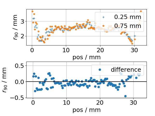
412                                        IEEE TRANSACTIONS ON RADIATION AND PLASMA MEDICAL SCIENCES, VOL. 2, NO. 5, SEPTEMBER 2018

The kNN algorithm can be speeded up by prepositioning                The sensor applies a configurable two-level trigger scheme to
events and searching the nearest neighbors only in a subset          detect and validate gamma particle interactions. Applying trig-
of the reference data [2]. However, the memory requirement           ger scheme 2, 2.33 detected photons are required on average
governed by the number of training events remain. Based on           to generate a trigger signal [20]. Then, a validation interval
the data given in [2], we estimate a memory requirement of           starts within which the second threshold has to be fulfilled.
more than 800 MB for a single detector stack of scintillator-        On average 17 photons need to be detected (validation set-
dimensions of 32 mm × 32 mm × 22 mm. Although it may                 ting 0x55:OR) to validate a trigger and start the integration
be possible to reduce the memory requirement for scintilla-          time [20]. If one pixel validates, all four pixels of the cor-
tors of smaller height, this memory requirement is impractical       responding DPC are read out. The information of one DPC
for currently available FPGAs. Adding external memory would          are referred to as hit. As stated before, every DPC is inde-
overcome this, but would add further complexity in the system        pendent. Subsequently, not all 16 DPCs of the tile necessarily
design at higher costs, requires additional space and increases      trigger and validate the trigger generating hits, especially for
the power consumption. The increased power consumption and           low photon densities. The tile offers a neighbor logic feature
the space requirements are especially critical for highly inte-      to force a read-out of the whole tile [21]. Neighbor logic is
grated PET and PET/MR systems. Thus, it is of high interest          not applied to reduce dead time of the whole tile caused by
to find computationally efficient positioning algorithms with        inappropriate validations. More details of the sensor tile can
low memory requirements.                                             be found in [22].
   In this paper, we present a calibration method capa-
ble to utilize both parallel hole and fan beam collimated            B. Scintillator Crystals and Wrappings
data. Employing the fan beam collimator, a full calibration
                                                                        A monolithic LYSO crystal (Epic Crystals, Kunshan,
for planar positioning requires less than 1 h. We demon-
                                                                     Jiangsu, China) with a ground plane of 32 mm × 32 mm
strate a positioning method based on gradient tree boosting
                                                                     matching the active sensor tile area and 12 mm height was
(GTB) regression. GTB is a supervised machine learning
                                                                     studied. The crystal was wrapped with highly reflective Teflon
method building predictive models organized as an indepen-
                                                                     tape (Klinger, Idstein, Germany). The monolith was coupled to
dently evaluable set of chains of binary decisions (decision
                                                                     the tile with the two-component dielectric silicon gel Sylgard
trees). Thus, determining the position of an event is fully
                                                                     527 (Dow Corning, Midland, MI, USA). As coincidence detec-
parallelizable and computational efficient because only sim-
                                                                     tor, we used a 12 mm high pixelated array with a pitch of 1 mm
ple comparisons with two possible outcomes are evaluated.
                                                                     as employed in [23] and [24].
The positioning performance and memory requirement of the
trained models can be influenced during the training process.
An FPGA implementation is already shown while the memory             C. Collimator Setup
requirement of the models is the limiting factor to fit the avail-      The whole setup was placed in a light-tight temperature
able memory of the FPGA [16], [17]. We present two different         chamber. Small fans additionally cooled the photodetectors
optimization scenarios: one optimized for a high positioning         to 5 ◦ C. In a PET, respectively, PET/MR system, the cho-
performance and one to find the best positioning performance         sen temperature can be achieved with a liquid cooling system
for given memory restrictions.                                       as demonstrated for the Hyperion IID insert [1]. The detector
                                                                     under study was placed on the electrically driven two-axis
                        II. M ATERIALS                               translation stage LIMES 90 (OWIS, Staufen im Breisgau,
                                                                     Germany). The translation stage sends its position by a feed-
   We used the technology evaluation kit (TEK) of Philips
                                                                     back loop to a control PC. The maximum position repetition
Digital Photon Counting (PDPC) as a coincidence setup to
                                                                     error is specified as 2 µm by the manufacturer. Up to two 22 Na
read out two sensor tiles built up from DPC 3200-22 digital
                                                                     sources with an active diameter of 0.5 mm and an activity
photon counters. As exchangeable collimators, a parallel hole
                                                                     of approximately 10 MBq each were used with both colli-
as well as a fan beam collimator were utilized. A monolithic
                                                                     mators. The radioactive sodium salt is backed in epoxy and
LYSO crystal of 12 mm height was studied. For detecting coin-
                                                                     encapsulated in an acrylic cylinder of 25.4 mm diameter and
cidences, a pixelated array was chosen. The complete setup
                                                                     6 mm height. The coincidence setup was operated with two
was placed in a light-tight temperature chamber.
                                                                     exchangeable collimators.
                                                                        1) Parallel Hole Collimator: The parallel hole collimator
A. Photodetectors                                                    has a length of 51 mm and bore diameter of 0.5 mm. An
   We used an array, also referred to as tile, of 16 independent     additional lead shielding enclosing the collimator and sources
dSiPM DPC 3200-22 of dimensions of 32.6 mm × 32.6 mm                 suppresses random coincidences and scattered coincidences.
from PDPC [18]. Each DPC consists of four pixels resulting in        A detailed description and characterization of the parallel hole
a photosensor with 64 pixels and a pixel pitch of 4 mm. Each         collimator is given in [25].
pixel contains 3200 single photon avalanche diodes (SPAD)               2) Fan Beam Collimator: We present a newly developed
on an active area of 3.2 mm × 3.88 mm. Every SPAD is                 fan beam collimator with an adaptable beam width. The work-
connected to an individual logic circuit for charging and read-      ing principle is based on a bottom shielding and two shielding
out. We deactivated 10% of the noisiest SPADs to reduce the          cakes as shown in Fig. 1. The distance between shielding cakes
overall dark counts based on a dark count measurement [19].          and bottom shielding defines the beam width. To prevent a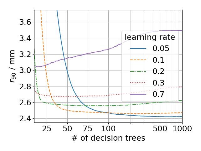
MÜLLER et al.: GTB-BASED POSITIONING METHOD FOR MONOLITHIC SCINTILLATOR CRYSTALS IN PET                                                        413

                                                                                detector position x. The beam profile b(x) is the derivative of
                                                                                the measured rate m(x). With discrete measurement points xi ,
                                                                                discrete derivation of the count rate m(x) leads to
                                                                                                                    m(xi+i ) − m(xi )
                                                                                          bi := b((xi + xi+1 )/2) =                   .
                                                                                                                       xi+i − xi
                                                                                   The obtained beam profile is described using a Gaussian fit.
                                                                                At the maximum of the beam profile, half of the beam covers
                                                                                the crystal. This point was assigned as the edge of the crystal.
                                                                                Using this method, the coordinate system of the stepper motor
                                                                                was aligned with a crystal coordinate system.
Fig. 1. Principle of the fan beam collimator. Side view: the distance between
bottom shielding and shielding cakes defines the beam width. Top view: the
geometrical shape of the shielding cakes restrict the span of the fan beam.     B. Data Acquisition and Preprocessing
The coincidence detector determines the area of the coincident beam inside         All measurements were conducted at a tile temperature
the fan beam.
                                                                                of 5 ◦ C. The data acquisition process depends on the uti-
                                                                                lized collimator. In all cases, the edges of the crystal were
                                                                                determined by the method explained in the previous section.
                                                                                For the parallel hole collimator, the crystal was irradiated at
                                                                                defined positions on a 2-D equidistant and perpendicular grid
                                                                                of 0.75 mm pitch. Thus, the calibration included 1849 points
                                                                                over the crystal surface. Using the fan beam collimator, parallel
                                                                                lines of 0.25 mm pitch were irradiated. Then, the crystal was
                                                                                rotated by 90◦ and the calibration was repeated. This results
                                                                                in a total of 256 line measurements. For a pitch of 0.75 mm,
                                                                                only 86 line measurements are required.
                                                                                   For later analysis, the recorded data was preprocessed as
                                                                                described in the following employing a tool developed in this
                                                                                group by Schug et al. [23]. For both detectors, a gamma
Fig. 2. Mechanical realization of the fan beam collimator as three-quarter
section view. Four screws maintain the distance between bottom shielding and
                                                                                interaction generates up to 16 hits. The hits related to one
each shielding cake. An additional top shielding reduces scatter events and     gamma interaction are merged and called a cluster. The
shields the sources. The source alignment tool hosts the radioactive sources    assigned timestamp of the cluster is the timestamp of the ear-
inside the collimator.
                                                                                liest hit. We used a cluster window of 40 ns to merge the
                                                                                hits. The TEK setup allows to apply a coincidence window
loss of coincident gammas by unintended absorptions, a larger                   on the DPC hits during the measurement. We applied a coin-
beam width was preventively chosen for the coincidence detec-                   cidence window of 40 ns for the hits in the TEK setup to
tor. The maximal span of the fan beam of 5 cm when exiting                      account for the cluster window needed afterward. Then, coin-
the lead block is defined by the geometrical shape of the                       cident clusters were searched employing a sliding coincidence
shielding cakes.                                                                window of 20 ns. To distinguish pixels missing in a cluster
   The mechanical realization additionally contains a top                       from a zero photoncount, missing pixels are marked with a
shielding and a source alignment tool (see Fig. 2). The source                  negative value. Missing pixels can be identified because the
alignment tool aligns the active area of the sources to one line                corresponding DPCs do not generate a hit and are not present
parallel to the slit and changes the height of this line in the                 while merging to clusters.
beam slit. To maintain the distance, each cake is equipped with                    We discarded clusters with a total photoncount below a
four screws with a metric fine pitch thread of 0.5 mm/turn. The                 threshold of 700 photons to reject noise. Based on the obtained
excess length of the screws can be varied between 0 mm and                      photon distribution, this equals an energy threshold of approx-
14 mm. A dial indicator of 0.01 mm precision was used to                        imately 290 keV. On average, 10% of all clusters with the
determine the excess length. In order to minimize scattering,                   lowest photoncount were ignored. Qualified clusters are called
the screws are positioned outside of the direct beam path.                      events. No further quality cuts were applied.
                                                                                   The recorded data was separated in three data sets: 1) train-
                                                                                ing data to train GTB models; 2) validation data to tune the
                            III. M ETHODS
                                                                                hyperparameters of GTB models (validation); and 3) test data
A. Beam Characterization                                                        to finally determine the positioning performance of trained
   We determined the beam profile as described by                               GTB models (evaluation). The number of events per irradiation
Ritzer et al. [25] as well as the coincidence rate: while mov-                  position and the pitch of irradiation positions of the training
ing the target detector step-wise into the beam, the coincidence                data were varied in the following (see Section III-D1). At max-
count rate of the setup is measured. The integral flux across                   imum, 10 000 events per irradiation position for the fan beam
the part of the beam profile already illuminating the scintil-                  collimator and 1000 events per irradiation position for the par-
lator is described by the measured coincidence rate m(x) at                     allel hole collimator were used. In all cases, validation and test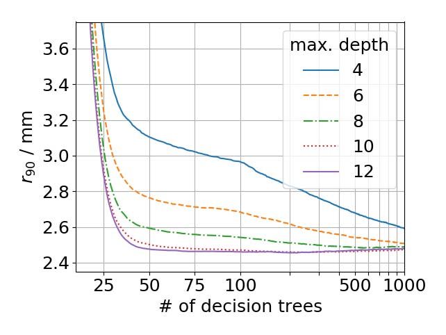
414                                         IEEE TRANSACTIONS ON RADIATION AND PLASMA MEDICAL SCIENCES, VOL. 2, NO. 5, SEPTEMBER 2018

                              TABLE I
    I NPUT C OMBINATIONS AND T HEIR I NCLUDED F EATURES . T HE CF      1) Bias Vector: The bias vector represents the mean posi-
  I NCLUDE COG, M AIN D IE , M AIN P IXEL , ROW AND C OLUMN S UMS         tioning error at a given position. In general, the distribu-
                                                                          tion of the bias vector magnitude follows no Gaussian
                                                                          profile due to edge effects. Thus, we report the median
                                                                          and the 90th percentile of the bias vector magnitude dis-
                                                                          tribution probing the central region and the tails of the
                                                                          distribution, respectively.
                                                                       2) SR: The SR is defined as the full width at half maxi-
                                                                          mum of the projected PSF or LSF. The fitting procedure
                                                                          was performed in accordance to the NEMA NU 4-2008
data contained events of the finest measured grid of 0.25 mm.             standard [29]. The SR is not sensitive to bias vector
Both validation and test data set consisted of 1250 events per            effects.
irradiation position for the fan beam collimator and 125 events        3) Intrinsic Spatial Resolution (SR*): The SR* is an esti-
per irradiation position for the parallel hole collimator.                mate for the intrinsic detector resolution. We corrected
   As described in more detail later on, GTB is able to han-              the SR by quadratically subtracting the finite beam
dle arbitrary input features and to recognize their respective            diameter determined as described in Section III-A.
information content. Hence, we tested the influence of sev-            4) Percentile Radius rx : The percentile radius rx is the
eral input features based on the raw data of the DPCs as well             radius enclosing the given percentile x of all assigned
as physically motivated features calculated from the raw DPC              events around the true irradiation position. Thus, the
data and their combination on the positioning performance (see            percentile radius is sensitive to the bias vector. For per-
Table I).                                                                 centile radii based on PSF, the Euclidean distance is
   In some cases and system designs, it can be beneficial to              employed with no projection needed. As for the bias
reduce the number of input features as demonstrated and dis-              vector distribution, we report the r50 and the r90 .
cussed in [26]. We used principal component analysis (PCA) to          5) Score of Radius 1.5 mm: The score value is the fraction
reduce the 64 pixel counts to 16 values. On average, these 16             of correctly assigned events. An event is called correctly
values represented 80% of the total information for our data.             assigned if it is found within the given radius of 1.5 mm
Details on PCA and the used scikit-learn implementation can               around the collimator position. As the percentile radius,
be found in [27] and [28].                                                the score value is sensitive to the bias vector.
   Statistical positioning algorithms have no information about
the physical properties of the given problem. For example,           D. Gradient Tree Boosting Position Estimation
the center of gravity (COG) is strongly correlated with the
interaction position of the gamma particle. Using such fea-             As a supervised machine learning technique, GTB employs
tures or adding them to the raw data can be beneficial for the       training data with known irradiation positions to build
positioning performance of the GTB models. We defined a set          predictive regression models. In the following, the main
of features referred to as calculated features (CF) in the fol-      aspects of the algorithm are described using a toy model of a
lowing. The CF contained index numbers of DPC and pixel              1-D crystal coupled to a four-channel photosensor made up of
with the highest photon count (main DPC and main pixel),             two 1-D DPCs with two channels each [see Fig. 3(a)]. Detailed
the COG position as well as the row and column sums. It is           reviews of decision trees and gradient boosting can be found
emphasized that all CF can directly be calculated on base of         in [30] and [31]. A mathematical description of the employed
the raw data, no further information are required. Missing DPC       XGBoost implementation is given in [32].
hit information in an event influences both the CFs and PCA             Like many other machine learning algorithms, GTB tends
leading to an uncertainty or jitter. The GTB needs to detect         to a phenomenon called overfitting; the residual variation as
this uncertainty and to adapt it during the training process.        it was part of the underlying set of training data is introduced
                                                                     into the model, decreasing the performance of the predictions
                                                                     on unknown data [33]. To avoid overfitting effects, the hyper-
C. Performance Parameters                                            parameters of the GTB models introduced in the following
   We used several parameters to test and characterize the           were tuned with the validation data test. The final evaluation of
performance of the positioning models. Using the parallel hole       the positioning performance was based on the test data set not
collimator, the performance parameters are based on the point        invoked either in training nor in validation of the GTB mod-
spread function (PSF) of the detector response. The PSF is           els. Both validation and evaluation employed the performance
defined as the 2-D distribution of the positioning errors in         parameters described before.
both x- and y-direction. Using a fan beam collimator, only              Trained GTB models are ensembles of so-called decision
one of the spatial coordinates is known from the collimator          trees [see Fig. 3(b)]. The ensemble is trained in an additive
position. Thus, performance parameters are calculated based          manner: the first decision tree is based on the given irradiation
on the line spread function (LSF) of the detector defined as         position. Every following decision tree is trained on the resid-
the 1-D positioning error distribution. The known collimator         uals of the previous ensemble (irradiation position–estimated
position defines the true position of an event. The following        position). Thus, every newly added decision tree corrects the
performance parameters are employed.                                 results of the previous ensemble. We use an additional factor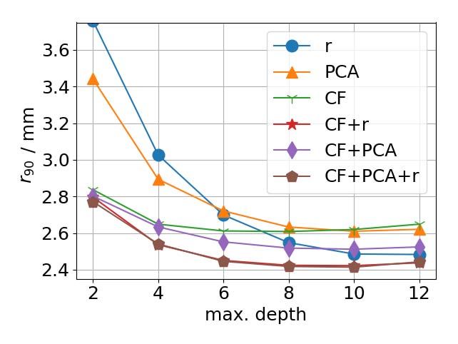
MÜLLER et al.: GTB-BASED POSITIONING METHOD FOR MONOLITHIC SCINTILLATOR CRYSTALS IN PET                                                                         415

                         (a)                                                                (b)

                                                 (c)                                                                                (d)

Fig. 3. Illustration of gradient tree boosting. (a) A 1-D crystal is coupled to a four-channel photosensor. Each two pixels are grouped to one DPC in this
example. The listed input features are used to train a GTB model with the interaction position as output. (b) The trained GTB models contain two decision
trees. Every decision tree is a sequential chain of binary decisions leading to a prediction. The second decision tree corrects the prediction of the first one. (c)
Two evaluation examples are shown and the results employing the GTB model in (b). Both decision trees can be evaluated in parallel. The final prediction is
the sum of all predictions of the ensemble. (d) Estimation of the memory requirement of a node and a leaf employing C standard library data types.

(< 1) called learning rate scaling the residuals and thereby                       information content from the provided set of input features.
the references for the next training. A smaller learning rate                      Features with low information content, for example, caused by
reduces the influence of a single tree leaving space for fur-                      uncertainty or jitter as mentioned before, are less likely to be
ther optimization. Decreasing the learning rates improves the                      considered. In our example, the main DPC is used earlier than
performance of trained models at the cost of needing a larger                      single photon counts due to the higher information content.
number of decision trees [34].                                                        GTB handles missing features in both training models and
   Every single decision tree is a sequential model combining                      prediction of events. Thus, nearly all data including partially
a chain of binary decisions (node) leading to a prediction [leaf,                  read out clusters can be used for calibration and position-
see Fig. 3(b)]. A single node evaluates one input variable with                    ing reducing the required calibration times. In case of sensors
a single split value. The maximum number of binary decisions                       which are self-triggering and validating on pixel level, a trig-
in a single decision tree is called maximum depth d. While                         ger caused by dark counts leads to a validation phase. During
the training is an additive process, the final decision trees can                  this validation phase, triggers of a real gamma interaction can-
be completely independently evaluated in parallel to find the                      not be detected causing a dead time. This reduces the rate of
position of an event under test. The final prediction is the sum                   events with information of all pixels present. Using a position-
of all predictions of the ensemble [see evaluation examples                        ing algorithm able to handle such events opens up the potential
in Fig. 3(c)]. Due to the additive training based on residuals,                    to reduce dead-time effects and to increase the sensitivity of a
the corrections get smaller for decision trees of higher order.                    system compared to algorithms requiring complete data such
In the given example, the decision trees output a prediction                       as standard kNN-implementations.
for the interaction position of the gamma based on the input                          As motivated before, the future goal is an implementation
features such as the photon counts and the COG.                                    of trained GTB in FPGAs. The feasibility of an implementa-
   Comparable to the ensemble, every single decision tree is                       tion is already shown while the memory requirement of the
trained in an additive manner as well. The algorithm starts with                   models is the limiting factor to fit the available memory of
the first node and greedily adds these new nodes improving                         the FPGA [16], [17]. C data types of the standard library are
the objective loss function of current decision tree most. The                     used to estimate the memory requirement. Further optimization
root mean squared error (RMSE) is employed as objective loss                       might be possible when using optimized data types for an
function. No further nodes are added if the maximum depth                          FPGA implementation. A single node object requires a total
is reached or the improvement is not justified compared to                         of 11 B and a leaf object 6 B [see Fig. 3(d)]. The number
the higher complexity penalized by a loss function. In this                        of nodes is less than or equal to 2d − 1. At maximum, 2d
way, GTB automatically chooses the features with the highest                       leaves are present. Thus, the total memory requirement MR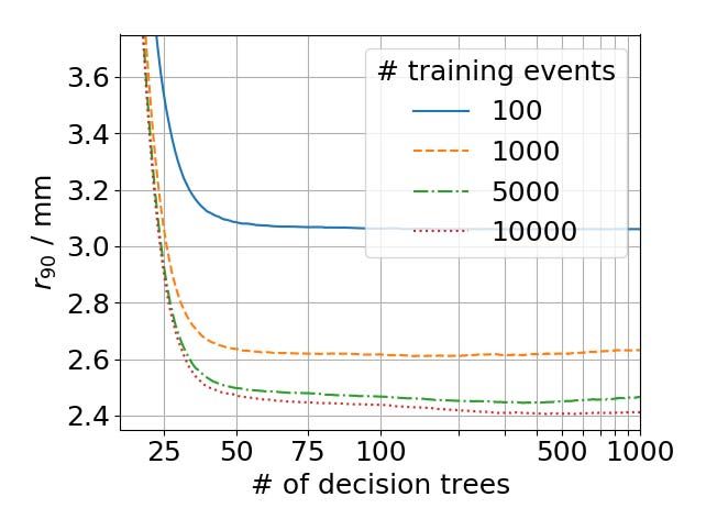
416                                        IEEE TRANSACTIONS ON RADIATION AND PLASMA MEDICAL SCIENCES, VOL. 2, NO. 5, SEPTEMBER 2018

                                                                                                  TABLE II
of a single decision tree is                                                   U SED B EAM W IDTHS AND C OINCIDENCE R ATES OF
                                                                               PARALLEL H OLE AND FAN B EAM C OLLIMATOR
            MR(d) = 2d − 1 · 11 B + 2d · 6 B.                  (1)

   The training and output of one GTB model is strictly 1-D
and completely independent for every direction. Therefore,
two separate models for x- and y-direction are needed.
Subsequently, both positioning steps are parallelizable in a
system architecture. The separation of both positioning direc-
tions enables the use of a fan beam collimator.
   The introduced hyperparameters, number of decision trees,
maximum depth, learning rate, and the input features directly         1-D functions. The course of all performance parameters was
influence the performance and the memory requirement of               discretely derived with respect to the number of decision trees.
GTB models. In the following, their effect is discussed and two       The first intersections with the ordinate axis were searched for
optimization scenarios are described: 1) a high-performance           every performance parameter excluding the SR (see Section V)
optimization without considering the memory requirements              leading to a list of numbers of decision trees. Then, starting for
and 2) an optimization process to find the best performing            the highest number of decision trees, the other parameters were
models fulfilling given memory-requirement restrictions.              tested for overfitting effects. A performance parameter was
   1) General Optimization Process: We developed a proto-             assumed to be overfitting if the derivative was positive (nega-
col to study the influence of several parameters which can be         tive for the score value). In case one parameter was overfitting,
divided up into three areas: 1) the measurement process (bin-         the next highest number of decision trees was tested repeating
ning of the calibration grid, number of events per calibration        the procedure. The final evaluation of the GTB models was
point); 2) the algorithm hyperparameters (number of decision          performed using the test data.
trees, maximum depth, learning rate); and 3) the input parame-           3) Memory-Requirement-Performance Optimization: The
ters (as defined in Table I). Trained models were verified based      limiting factor for an FPGA implementation is the memory
on all defined performance parameters with the validation data        requirement of trained models as described before. Thus, it is
to avoid overfitting. First, we randomly tested different com-        of high interest to find the best performing models for given
binations of the given parameters to find a suitable start point      memory resources. Employing the same set of parameters as
for the following process. The parameter ranges for the initial       listed above (see Section III-D2), we trained models for dif-
search were adapted to suggestions found in [31]. The course          ferent learning rates and maximum depths. In contrast to the
off all performance parameters as well as the objective loss          high-performance-optimization, an empirically suitable con-
function of the GTB models were plotted against the num-              vergence criterion based on the r90 determined the number of
ber of decision trees to check the dependencies between the           decision trees in the ensemble: the number of decision trees
single parameters. Second, always one of the listed parame-           was fixed if the newly added decision tree improved the aver-
ters was varied keeping all other parameters constant. For all        aged r90 less than 0.01 mm. The r90 and the SR were plotted
parameters regarding the measurement process and the algo-            for all found models against the memory requirement allowing
rithm parameters, GTB models for up to 1000 decision trees            to find the best suitable models.
were trained. For the different input features, GTB models of a
fixed number of decision trees were trained varying the maxi-                                  IV. R ESULTS
mum depths. Based on the variation of the maximum depth, an           A. Beam Characterization
ensemble size of 100 decision trees was selected. We chose to            The results of the beam characterization are summarized
present the averaged 90th percentile radius as validation met-        in Table II. The parallel hole collimator reached a coinci-
ric to include bias effects and to be sensitive to the tails of the   dence rate of 24s−1 and the fan beam collimator of 199s−1
LSF or PSF, respectively.                                             for a significant narrower beam width which equals a factor
   2) High-Performance Optimization: Based on the results of          of about 8.
the general optimization process (see Section V), the binning
of the calibration grid was set to 0.75 mm, the number of             B. Data Acquisition
training events to 5000 for the fan beam collimator (250 for
the parallel hole collimator) per irradiation position and the           Taking all irradiation positions into account, the photopeak
input set to CFs and raw data (CF+r). Then, we conducted              position calculated based on the total photonsum was found
an exhaustive search validating all possible combinations of          for 1240 photons with an FWHM of 396 photons which
the algorithm hyperparameters: The discrete hyperparameters,          equals an energy resolution of approximately 32 %. Fig. 4
number of decision trees and maximum depth, were varied               shows obtained read-out characteristics with a Gaussian fit.
ranging from 1 to 1000 and from 4 to 12 by steps of 1, respec-        The Gaussian distribution describes the data well.
tively. The continuous learning rate was probed for the values
[0.05, 0.1, 0.2, 0.3, 0.4, 0.7].                                      C. General Optimization Process
   To select the GTB models of the best positioning                     The randomized parameter search lead to a maximum depth
performance, we adapted the classical optimization problem of         of 10, a learning rate of 0.1 and raw data of 5000 training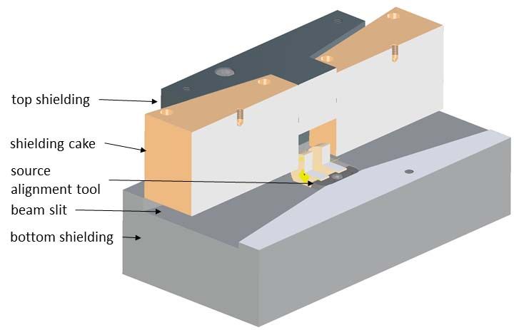
MÜLLER et al.: GTB-BASED POSITIONING METHOD FOR MONOLITHIC SCINTILLATOR CRYSTALS IN PET 417
respective optima. Fig. 6(b) displays the r90 as a function of
the irradiation position for the coarse and the fine calibration
grid. In the upper plot, both distributions are showing a very
similar course. Their characteristics are the same in general
including the behavior at the edges. A significant improve-
ment of the r90 is observed close to 3 mm and 29 mm for both
pitches of the calibration grid. The lower plot displays the dif-
ference between the corresponding r90 distributions fluctuating
unsystematically around 0.
In case the number of training data is increased, the model
performance improves until a sufficient amount of data is given
[see Fig. 6(c)]. After this point, just small improvements can
Fig. 4. Histogram and Gaussian fit (dashed line) of read out DPCs for events be observed if further training data are added. As an example,
acquired by a homogeneous illumination of the crystal surface.
doubling the training events from 5000 to 10 000 per calibra-
tion point boosts the r90 by less than 1.5% evaluated at their
respective optima.
The positioning performance of the models increases for
larger maximum depths [see Fig. 6(d)]. Increasing step-wise
the maximum depth, the performance-boost gets less toward a
maximum depth of 10. For even higher maximum depths, no
further gain of the positioning performance is observed. The
positioning performance of the GTB models converges to a
global optimum point for a large number of decision trees as
visible toward 1000 decision tress.
For higher learning rates, the best positioning performance
of the respective GTB models is reached for a smaller num-
ber of decision trees [see Fig. 6(e)]. However, the positioning
performance deteriorates compared with the models employing
a smaller learning rate. This is clearly visible for the learn-
ing rate of 0.7. Less than 10 decision trees are needed to
reach the optimum point. However, the maximum performance
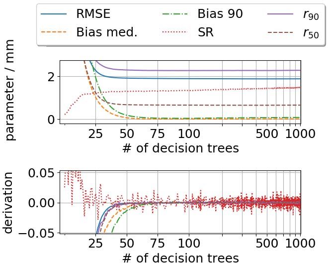
Fig. 5. Performance parameters and the objective loss function (RMSE) of
the GTB models (top) and their discrete derivative (down) against the number is reduced about 20% compared to a learning rate of 0.05
of decision trees. The abscissa is plotted linear up to 100 decision trees and evaluated at their respective optima.
logarithmic afterward. A maximum depth of 10 and a learning rate of 0.1 In general, the performance increases for all evaluated com-
were applied with raw data as input. The course of all shown performance
parameters is strongly correlated. The SR increases with a higher number binations of input features except CF increasing the maximum
of decision trees. The derivative of the SR has the highest fluctuation of all depth up to 10 [see Fig. 6(f)]. For a depth of 12, only raw
performance parameters. data as input lead to a slightly better performance. The other
input combinations do not improve or slightly deteriorate.
For maximum depths up to 6, all input combinations includ-
events acquired every 0.75 mm as start point for the training ing CF lead to better results than raw data. For maximum
process. The GTB objective loss function RSME is strongly depths larger than 6, models trained with raw data increase
correlated with all performance parameters (see Fig. 5). All their performance compared to CF, PCA and combination
performance parameters except the SR continuously decrease CF+PCA. Combination CF+r and combination CF+PCA+r
until their optimum is reached. Their derivatives tends to 0 have almost the same characteristics.
with a decreasing slope for a higher number of decision trees.
After their optimum, the performance parameters fluctuate or
worsen again. The SR increases adding more decision trees
especially up to about 25 decision trees. The derivative of the D. High-Performance Optimization
SR is neither continuous nor monotonous. The best positioning performance was found for GTB mod-
Results of the general optimization process of the fan els of maximum depth 10, learning rate 0.1 and 71 to 77
beam calibration along one direction are exemplarily shown in decision trees requiring in total around 2 MB of memory
Fig. 6. We used the found start point for the training process for both planar directions. 2-D spatial distributions of the
if not stated otherwise. bias vector and r50 are shown for the parallel hole cali-
The GTB models show a very similar course of the r90 for bration in Fig. 7. The bias vector is randomly distributed
all studied pitches ranging from 0.25 mm to 0.75 mm of the in the central region of the crystal. At the edges, a bias
calibration grid [see Fig. 6(a)]. The performance increases less toward the center is observed. The r50 is homogeneously dis-
than 2% for those models trained with the finest available irra- tributed in the central region and deteriorates toward the crystal
diation pitch compared to the coarsest one evaluated at their edges.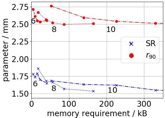
418                                                IEEE TRANSACTIONS ON RADIATION AND PLASMA MEDICAL SCIENCES, VOL. 2, NO. 5, SEPTEMBER 2018

                             (a)                                                 (b)                                                (c)

                             (d)                                                 (e)                                                (f)

Fig. 6. Exemplary optimization process for data measured with the fan beam collimator. Unless stated otherwise, ensembles of maximum depth 10 and
learning rate 0.1 are trained on raw data of 5000 training events per position on a calibration grid of 0.75 mm pitch. The test data have a pitch of 0.25 mm. In
case the number of decision trees is shown on the abscissa, a linear scale is chosen up to 100 decision trees and a logarithmic scale afterward. (a) Averaged
r90 against the number of decision trees varied for the pitch of the calibration grid. (b) Spatial r90 -distributions for models trained with calibration grids
of 0.25 mm and 0.75 mm, respectively. Top: both r90 -distributions as overlay. Down: difference of the distributions. (c) Averaged r90 against the number
of decision trees varied for the number of training events per position. (d) Averaged r90 against number of decision trees for different maximum depths.
(e) Averaged r90 against number of decision trees for different learning rates. (f) Averaged r90 against the maximum depth for different input combinations
(see Table I). All models consist of 70 decision trees.

                                            (a)                                                                 (b)

Fig. 7. Exemplary spatial distribution of the parallel hole collimator calibration based on the GTB models of the best positioning performance. (a) Bias
vector distribution. The color scale represents the bias vector magnitude. (b) r50 distribution.

   Table III shows the performance parameters for calibrations                   E. Memory-Requirement-Performance Optimization
of both parallel hole and fan beam collimator. In general, the                      Fig. 8 exemplarily shows the SR and r90 for possible GTB
performance parameters of both calibration methods probing                       models against the memory requirement for the calibration
the central area of the LSF lead to very similar results. The                    in y-direction of the crystal. Every chosen maximum depth
r90 is around 6% better for the fan beam calibration. For both                   (denoted next to each line) is probed for several learning rates
calibrations method, an SR* of 1.40 mm FWHM or better is                         resulting in a specific number of decision trees defined by the
achieved.                                                                        convergence criterion and plotted as one line. For more clarity,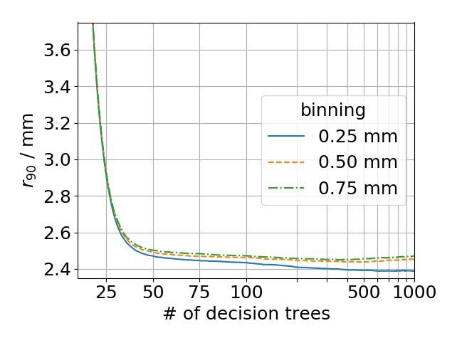
MÜLLER et al.: GTB-BASED POSITIONING METHOD FOR MONOLITHIC SCINTILLATOR CRYSTALS IN PET                                                        419

                           TABLE III
 OVERVIEW OF THE B EST ACHIEVED P OSITIONING P ERFORMANCE FOR                     The photon densities in the employed monolith are too low
    PARALLEL H OLE AND FAN B EAM C OLLIMATED C ALIBRATION .                    to generate a significant amount of events with hits of all
      F OR THE PARALLEL H OLE C ALIBRATION , P ERFORMANCE                      16 DPCs present (see Fig. 4). In only 0.038% of all cases,
        PARAMETERS BASED ON THE PSF A RE G IVEN A S T OT
                                                                               the events include hits of all 16 DPCs. This emphasizes the
                                                                               need for a calibration and positioning algorithm that is able to
                                                                               handle missing data.
                                                                                  The general optimization process shows the connections
                                                                               between the performance parameters and the influence of the
                                                                               algorithm parameters. The course of the SR is not as stable as
                                                                               these of the other defined performance parameters (see Fig. 5).
                                                                               As the determination procedure of the SR includes a projec-
                                                                               tion and a binning process, the SR can be affected by binning
                                                                               artifacts. Thus, the SR is not suitable for determination of the
                                                                               GTB models with the best positioning performance. In the
                                                                               region of a small number of decision trees (up to about 25
                                                                               decision trees in the shown example), the SR has very small
                                                                               values and worsens for increasing model ensembles. At the
                                                                               beginning of the training process, the possible predictions of
                                                                               GTB models are limited to the number of leafs. Subsequently,
                                                                               the predictions are discrete which is beneficial for the SR.
                                                                               Increasing the number of decision trees, more predictions are
                                                                               possible increasing the general positioning performance of the
                                                                               model while deteriorating the SR.
                                                                                  Fig. 6(a) and (b) demonstrates that the GTB algorithm
                                                                               builds reliable regression models. Thus, the number of cal-
Fig. 8. Planar positioning performance calibrated in the y-direction of the    ibration points and the calibration time needed can be
crystal against memory requirement. The numbers next to the lines denote the   reduced without compromising too much on the positioning
maximum depth of the models.
                                                                               performance. Therefore, a pitch of 0.75 mm of the calibration
                                                                               grid is employed for the training data. Most other calibra-
                                                                               tion methods found in literature employ a calibration grid of
the results of selected maximum depths are shown. For a
                                                                               0.25 mm [2], [4], [9], [15]. Thus, GTB allows to reduce the
given amount of memory, multiple combinations of maximum
                                                                               calibration time by a factor of 3 for the fan beam collimator
depth and learning rate fulfill possible memory restrictions.
                                                                               keeping the number of training events per irradiation position
For maximum depths of 6 and 8, the r90 deteriorates while
                                                                               constant. The course of the r90 toward the scintillator surfaces
the SR still improves. GTB models of maximum depth 8
                                                                               is based on two effects: very close to the surfaces, the bias
obtain a similar positioning performance compared to GTB
                                                                               vector dominates the r90 and leads to a deterioration. Near the
models of maximum depth 10 with significantly less memory
                                                                               positions of 3 mm and 29 mm, the bias vector has vanished
requirements.
                                                                               while the photon pattern is still affected by the reflections
                                                                               of the scintillator surfaces. These reflections have a higher
                           V. D ISCUSSION                                      flux compared to reflections at the surfaces caused by gamma
   The used method for beam characterization works well and                    interactions at central irradiation positions due to geometri-
allows a reliable determination of the crystal edges. The beam                 cal aspects. Thus, the reflections of gamma interactions close
widths are larger than the bore diameter and the slit width,                   to the surfaces are not part of a uniform background. This
respectively. The beam spreads as a function of the distance                   leads to more distinct photon patterns compared to central
between collimator and detector caused by geometrical effects                  positions of the crystal which is beneficial for the position-
and Compton-scatter of gamma particles with the collimator.                    ing performance of GTB models. Furthermore, the maximum
   The given characteristics of the photon distribution indicate               width of the r90 distribution is geometrically limited by the
that no photopeak events are excluded for training and testing                 scintillator surfaces. This effect is also beneficial for the r90 .
the GTB models. Due to missing hit information in events,                         Beside the number of irradiation positions, the number of
the total photonsum is no stable energy criterion. Thus, the                   training events is directly proportional to the measurement
obtained photon distribution is not suitable for an energy cali-               time. As shown in Fig. 6(c), no significant increase in the
bration leading to good energy resolutions. A dedicated energy                 positioning performance for more than 5000 training events
calibration needs to account for the missing hit information.                  is observed for the fan beam calibration. The GTB algorithm
Furthermore, the scintillator should be divided up into voxels                 finds all causal connections in the data within this data set size.
with their own energy calibration to include spatial variations                We set the number of training events per irradiation position
in the characteristics of the detector. Currently, we are investi-             to 5000 for the fan beam calibration and to 250 for the parallel
gating a dedicated energy calibration which is not in the scope                hole calibration. This leads to a calibration time of less than
of this paper.                                                                 1 h for both planar directions for the fan beam calibration and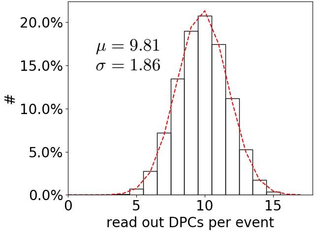
420                                       IEEE TRANSACTIONS ON RADIATION AND PLASMA MEDICAL SCIENCES, VOL. 2, NO. 5, SEPTEMBER 2018

1 d for the parallel hole collimator. The GTB algorithm offers      the adaptability of the GTB algorithm. The memory require-
the possibility to further reduce the measurement time while        ment can be adjusted by modifying the discussed parameters.
still providing reliable positioning models.                        The memory requirement of the models is orders of magnitude
    Maximum depths larger than 10 are not reasonable for the        lower compared to our estimates of 4 MB of an ML or 800 MB
presented geometry as they do not lead to a further improved        of a kNN implementation based on data of [2] and [11].
accuracy [see Fig. 6(d)]. For an FPGA implementation, the           For example, employing the shown model of maximum depth
maximum depth is the most critical parameter because the            6 and 16 kB memory requirement (32 kB for both directions),
memory requirement is O(n2d ) with d the maximum depth              the SR is around 1.7 mm which outperforms most pixelated
and n the number of decision trees.                                 clinical detector blocks used in whole-body PET [35].
    A high learning rate can be used to create well-performing
positioning models with a low memory requirement. GTB
                                                                                              VI. C ONCLUSION
models with a large learning rate tend faster to overfitting
effects and perform worse compared to those models trained             The presented GTB-based positioning algorithm allows a
with small learning rates.                                          time-efficient calibration and is able to create positioning mod-
    All models containing CF as input features show a signif-       els suitable to be implemented on an FPGA. Compared to a
icant increased performance compared to input combinations          parallel hole collimator, the developed fan beam collimator
without them. The GTB algorithm efficiently utilizes the phys-      accelerates the full planar positioning calibration by a factor
ical information provided by the chosen set of CF and also          of 20 to less than 1 h. Our developed positioning algorithm
accounts for the uncertainties caused by missing hit infor-         flexibly handles different input features and their combinations
mation. Especially for models of a small maximum depth,             including PCA transformed data. Calibrations with parallel
the CF are easier to interpret. For higher maximum depths,          hole and fan beam collimator lead to equivalent results. GTB
the GTB model has “learned” causal connections between the          accepts missing features for training and prediction which
raw data and is able to outperform the CF. However, adding          is beneficial for sensitivity in PET systems. Additional fea-
CF to the raw data as input still improves the performance          tures based on physical properties such as the first moment
due to additional information content. Input combinations PCA       (COG) significantly improve the positioning performance. The
and PCA+r perform worse than those input combinations con-          flexibility of handling all kind of input features enables pos-
taining raw data due to the information loss of the PCA. As         sibly future optimizations. We trained GTB models for two
mentioned before, 80% of the information are preserved in the       scenarios demonstrating the versatility of the algorithm: one
first 16 PCA components. However, this demonstrates that the        without compromising on positioning performance and one
GTB models are able to handle PCA transformed input fea-            optimizing the positioning performance for a given memory
tures. Input combinations CF+PCA+r shows no performance             restriction. For a 12 mm high monolithic block, we achieved
boost compared to CF+r because the PCA does not add                 an SR of 1.24 mm FHWM and 1.40 mm FWHM for y- and
additional information to the training process.                     x-direction corrected for the finite beam size. Future work will
    GTB models show a homogeneous positioning performance           evaluate the applicability and performance of the algorithm to
over the whole central crystal region with the typical bias         DOI positioning as well as for different scintillator geome-
effects at the edges (see Fig. 7) found in monolithic scin-         tries. Furthermore, the aim of an FPGA implementation will
tillators. The r50 deteriorates at the crystal edges because this   be realized.
performance parameter is sensitive to bias vector effects.
    Calibrations based on parallel hole and fan beam instrumen-                                   R EFERENCES
tations work well and lead to very similar results. This is due
                                                                     [1] B. Weissler et al., “A digital preclinical PET/MRI insert and initial
to the fact that the used GTB models are only 1-D. A 2-D                 results,” IEEE Trans. Med. Imag., vol. 34, no. 11, pp. 2258–2270,
implementation might benefit from point data in the sense                Nov. 2015, doi: 10.1109/TMI.2015.2427993.
of a more efficient memory requirement. Small deviations             [2] G. Borghi, V. Tabacchini, and D. R. Schaart, “Towards monolithic
                                                                         scintillator based TOF-PET systems: Practical methods for detector cali-
in single performance parameters such as the r90 can origin              bration and operation,” Phys. Med. Biol., vol. 61, no. 13, pp. 4904–4928,
from the influence of the different size of the gamma beams.             Jul. 2016, doi: 10.1088/0031-9155/61/13/4904.
Furthermore, the rate of scattered gamma particles in the colli-     [3] H. T. Van Dam, G. Borghi, S. Seifert, and D. R. Schaart,
                                                                         “Sub-200 ps CRT in monolithic scintillator PET detectors using
mator may differ for both instrumentations. Considering these            digital SiPM arrays and maximum likelihood interaction time esti-
aspects, both calibration processes lead to nearly equivalent            mation,” Phys. Med. Biol., vol. 58, no. 10, pp. 3243–3257, 2013,
performances.                                                            doi: 10.1088/0031-9155/58/10/3243.
    Comparing the positioning performance in x- and y-               [4] P. Bruyndonckx et al., “Evaluation of machine learning algorithms for
                                                                         localization of photons in undivided scintillator blocks for PET detec-
direction (see Table III), the GTB models perform equivalently           tors,” IEEE Trans. Nucl. Sci., vol. 55, no. 3, pp. 918–924, Jun. 2008,
along both directions. Small deviations may occur due to                 doi: 10.1109/TNS.2008.922811.
statistical effects.                                                 [5] R. Marcinkowski, P. Mollet, R. Van Holen, and S. Vandenberghe, “Sub-
                                                                         millimetre DOI detector based on monolithic LYSO and digital SiPM
    Fig. 8 helps to select the best training and model param-            for a dedicated small-animal PET system,” Phys. Med. Biol., vol. 61,
eters for a given memory restriction. Taking both displayed              no. 5, pp. 2196–2212, 2016, doi: 10.1088/0031-9155/61/5/2196.
performance parameters into account, an optimum point for            [6] A. J. Gonzalez et al., “The MINDView brain PET detector, feasibility
                                                                         study based on SiPM arrays,” Nucl. Instrum. Methods Phys. Res. Section
every maximum depth can be chosen before overfitting effects             A Accelerators Spectrometers Detectors Assoc. Equipment, vol. 818,
occur. This optimization scenario demonstrates the potential of          pp. 82–90, May 2016, doi: 10.1016/j.nima.2016.02.046.
MÜLLER et al.: GTB-BASED POSITIONING METHOD FOR MONOLITHIC SCINTILLATOR CRYSTALS IN PET 421
[7] A. González-Montoro et al., “Detector block performance [19] T. Frach, G. Prescher, C. Degenhardt, and B. Zwaans, “The digital sili-
based on a monolithic LYSO crystal using a novel signal con photomultiplier—System architecture and performance evaluation,”
multiplexing method,” Nucl. Instrum. Methods Phys. Res. Section in Proc. IEEE Nucl. Sci. Symp. Med. Imag. Conf., IEEE, Oct. 2010,
A Accelerators Spectrometers Detectors Assoc. Equipment, Feb. 2018, pp. 1722–1727, doi: 10.1109/NSSMIC.2010.5874069.
doi: 10.1016/j.nima.2017.10.098. [20] V. Tabacchini, V. Westerwoudt, G. Borghi, S. Seifert, and D. R. Schaart,
[8] X. Li, C. Lockhart, T. K. Lewellen, and R. S. Miyaoka, “A high “Probabilities of triggering and validation in a digital silicon photo-
resolution, monolithic crystal, PET/MRI detector with DOI position- multiplier,” J. Instrum., vol. 9, no. 6, pp. P06016–P06016, Jun. 2014,
ing capability,” in Proc. Annu. Int. Conf. IEEE Eng. Med. Biol. Soc., doi: 10.1088/1748-0221/9/06/P06016.
vol. 2008. 2008, pp. 2287–2290, doi: 10.1109/IEMBS.2008.4649654. [21] D. Schug et al., “First evaluations of the neighbor logic of the digital
[9] H. T. Van Dam et al., “Improved nearest neighbor methods for gamma SiPM tile,” in Proc. IEEE Nucl. Sci. Symp. Med. Imag. Conf. Rec., IEEE,
photon interaction position determination in monolithic scintillator PET Oct. 2012, pp. 2817–2819, doi: 10.1109/NSSMIC.2012.6551642.
detectors,” IEEE Trans. Nucl. Sci., vol. 58, no. 5, pp. 2139–2147, [22] R. Marcinkowski, S. Espana, R. Van Holen, and S. Vandenberghe,
Oct. 2011, doi: 10.1109/TNS.2011.2150762. “Effects of dark counts on digital silicon photomultipliers performance,”
[10] A. González-Montoro et al., “Performance study of a large monolithic in Proc. IEEE Nucl. Sci. Symp. Med. Imag. Conf. (NSS/MIC), IEEE,
LYSO PET detector with accurate photon DOI using retroreflector lay- Oct. 2013, pp. 1–6, doi: 10.1109/NSSMIC.2013.6829323.
ers,” IEEE Trans. Radiat. Plasma Med. Sci., vol. 1, no. 3, pp. 229–237, [23] D. Schug et al., “Data processing for a high resolution preclinical PET
May 2017, doi: 10.1109/TRPMS.2017.2692819. detector based on philips DPC digital SiPMs,” IEEE Trans. Nucl. Sci.,
[11] S. España, R. Marcinkowski, V. Keereman, S. Vandenberghe, vol. 62, no. 3, pp. 669–678, Jun. 2015, doi: 10.1109/TNS.2015.2420578.
and R. Van Holen, “DigiPET: Sub-millimeter spatial resolution [24] N. Gross-Weege, D. Schug, P. Hallen, and V. Schulz, “Maximum like-
small-animal PET imaging using thin monolithic scintilla- lihood positioning algorithm for high-resolution PET scanners,” Med.
tors,” Phys. Med. Biol., vol. 59, no. 13, pp. 3405–3420, 2014, Phys., vol. 43, no. 6, pp. 3049–3061, 2016, doi: 10.1118/1.4950719.
doi: 10.1088/0031-9155/59/13/3405. [25] C. Ritzer, P. Hallen, D. Schug, and V. Schulz, “Intercrystal scat-
[12] P. Conde et al., “Determination of the interaction position of gamma ter rejection for pixelated PET detectors,” IEEE Trans. Radiat.
photons in monolithic scintillators using neural network fitting,” Plasma Med. Sci., vol. 1, no. 2, pp. 191–200, Mar. 2017,
IEEE Trans. Nucl. Sci., vol. 63, no. 1, pp. 30–36, Feb. 2016, doi: 10.1109/TNS.2017.2664921.
doi: 10.1109/TNS.2016.2515163. [26] L. A. Pierce et al., “Multiplexing strategies for monolithic crystal PET
[13] Y. Wang, W. Zhu, X. Cheng, and D. Li, “3D position estimation detector modules,” Phys. Med. Biol., vol. 59, no. 18, pp. 5347–5360,
using an artificial neural network for a continuous scintillator PET Sep. 2014, doi: 10.1088/0031-9155/59/18/5347.
detector,” Phys. Med. Biol., vol. 58, no. 5, pp. 1375–1390, Mar. 2013, [27] K. Pearson, “LIII. On lines and planes of closest fit to systems of points
doi: 10.1088/0031-9155/58/5/1375. in space,” London Edinburgh Dublin Philos. Mag. J. Sci., vol. 2, no. 11,
[14] G. Borghi, B. J. Peet, V. Tabacchini, and D. R. Schaart, “A 32 mm x pp. 559–572, 1901.
32 mm x 22 mm monolithic LYSO: Ce detector with dual-sided digital [28] F. Pedregosa et al., “Scikit-learn: Machine learning in python,” J. Mach.
photon counter readout for ultrahigh-performance TOF-PET and TOF- Learn. Res., vol. 12, pp. 2825–2830, Oct. 2011.
PET/MRI,” Phys. Med. Biol., vol. 61, no. 13, pp. 4929–4949, Jun. 2016, [29] Performance Measurements of Small Animal Positron Emission
doi: 10.1088/0031-9155/61/13/4929. Tomographs, NEMA Standard NU 4-2008, 2008.
[15] G. Borghi, V. Tabacchini, S. Seifert, and D. R. Schaart, “Experimental [30] S. B. Kotsiantis, “Decision trees: A recent overview,” Artif. Intell. Rev.,
validation of an efficient fan-beam calibration procedure for K- vol. 39, no. 4, pp. 261–283, 2013, doi: 10.1007/s10462-011-9272-4.
nearest neighbor position estimation in monolithic scintillator detec- [31] A. Natekin, A. Knoll, M.-O. Gewaltig, and O. Michel, “Gradient boost-
tors,” IEEE Trans. Nucl. Sci., vol. 62, no. 1, pp. 57–67, Feb. 2015, ing machines, a tutorial,” Front. Neurorobot., vol. 7, p. 21, Dec. 2013,
doi: 10.1109/TNS.2014.2375557. doi: 10.3389/fnbot.2013.00021.
[16] R. Kułaga and M. Gorgoń, “FPGA implementation of decision [32] T. Chen and C. Guestrin, “XGBoost: A scalable tree boosting system,”
trees and tree ensembles for character recognition in vivado HLS,” in Proc. 22nd ACM SIGKDD Int. Conf. Knowl. Disc. Data Min. (KDD),
Image Process. Commun., vol. 19, nos. 2–3, pp. 71–82, 2014, 2016, pp. 785–794, doi: 10.1145/2939672.2939785.
doi: 10.1515/ipc-2015-0012. [33] T. Dietterich, “Overfitting and undercomputing in machine learning,”
[17] B. Van Essen, C. Macaraeg, M. Gokhale, and R. Prenger, “Accelerating ACM Comput. Surveys, vol. 27, no. 3, pp. 326–327, 1995.
a random forest classifier: Multi-core, GP-GPU, or FPGA?” in Proc. [34] J. H. Friedman, “Greedy function approximation: A gradient
IEEE 20th Int. Symp. Field Program. Custom Comput. Mach., IEEE, boosting machine,” Ann. Stat., vol. 29, no. 5, pp. 1189–1232,
Apr. 2012, pp. 232–239, doi: 10.1109/FCCM.2012.47. 2001.
[18] C. Degenhardt et al., “The digital silicon photomultiplier—A novel sen- [35] G. B. Saha, Basics of PET Imaging: Physics, Chemistry,
sor for the detection of scintillation light,” in Proc. IEEE Nucl. Sci. Symp. and Regulations. Cham, Switzerland: Springer Int., 2015,
Conf. Rec., 2009, pp. 2383–2386, doi: 10.1109/NSSMIC.2009.5402190. doi: 10.1007/978-3-319-16423-6.You can also read