LAPACK Working Note #224 QR Factorization of Tall and Skinny Matrices in a Grid Computing Environment
←
→
Page content transcription
If your browser does not render page correctly, please read the page content below
LAPACK Working Note #224
QR Factorization of Tall and Skinny Matrices in a
         Grid Computing Environment
                         Emmanuel Agullo ∗ , Camille Coti † , Jack Dongarra ∗ ,
                               Thomas Herault ‡ , Julien Langou §
             ∗  Dpt of Electrical Engineering and Computer Science, University of Tennessee,
                 1122 Volunteer Blvd, Claxton Building, Knoxville, TN 37996-3450, USA
                           † INRIA Saclay-Île de France, F-91893 Orsay, France
                           ‡ Univ Paris Sud, University of Tennesse, LRI, INRIA
              § Dpt of Mathematical and Statistical Sciences, University of Colorado Denver,

                 Campus Box 170, P.O. Box 173364, Denver, Colorado 80217-3364, USA
                        eagullo@eecs.utk.edu, coti@lri.fr, dongarra@eecs.utk.edu,
                                 herault@lri.fr, julien.langou@ucdenver.edu

                                                           Abstract
           Previous studies have reported that common dense linear algebra operations do not achieve speed up by
      using multiple geographical sites of a computational grid. Because such operations are the building blocks
      of most scientific applications, conventional supercomputers are still strongly predominant in high-performance
      computing and the use of grids for speeding up large-scale scientific problems is limited to applications exhibiting
      parallelism at a higher level. We have identified two performance bottlenecks in the distributed memory algorithms
      implemented in ScaLAPACK, a state-of-the-art dense linear algebra library. First, because ScaLAPACK assumes
      a homogeneous communication network, the implementations of ScaLAPACK algorithms lack locality in their
      communication pattern. Second, the number of messages sent in the ScaLAPACK algorithms is significantly
      greater than other algorithms that trade flops for communication. In this paper, we present a new approach for
      computing a QR factorization – one of the main dense linear algebra kernels – of tall and skinny matrices in a grid
      computing environment that overcomes these two bottlenecks. Our contribution is to articulate a recently proposed
      algorithm (Communication Avoiding QR) with a topology-aware middleware (QCG-OMPI) in order to confine
      intensive communications (ScaLAPACK calls) within the different geographical sites. An experimental study
      conducted on the Grid’5000 platform shows that the resulting performance increases linearly with the number
      of geographical sites on large-scale problems (and is in particular consistently higher than ScaLAPACK’s).

                                            I. I NTRODUCTION
   Grid computing [20] as a utility has reached the mainstream. Many large-scale scientific problems have
been successfully solved thanks to the use of computational grids (or, simply, grids). These problems
cover a wide range of scientific disciplines including biology (protein folding [31]), medicine (cure
muscular dystrophy [9]), financial modeling, earthquake simulation, and climate/weather modeling.
Such scientific breakthroughs have relied on the tremendous processing power provided by grid in-
frastructures. For example, the Berkeley Open Infrastructure for Network Computing (BOINC) [3]
gathers the processing power of personal computers provided by people volunteering all over the
world. This processing power is then made available to researchers through different projects such as
Climateprediction.net [2], Rosetta@home [16] and World Community Grid (WCG)1 . As of September
2009, 18, BOINC had 566,000 active computers (hosts) worldwide for an average total processing power
  1
    This work was partly supported by the EC grant for the QosCosGrid project (grant # FP6-2005-IST-5 033883), and NSF-CCF (grant
#881520).
  1
    http://www.worldcommunitygrid.org
of 2.4 Pflop/s2 . Furthermore, following the supercomputing trends, grid computing infrastructures have
successfully exploited the emerging hardware technologies. The Folding@Home project [7] – which
aims at understanding protein folding, misfolding, and related diseases – achieves 7.9 Pflop/s thanks
to grid exploiting specialized hardware such as graphics processing units (GPUs), multicore chips and
IBM Cell processors.
However, conventional supercomputers are strongly predominant in high-performance computing
(HPC) because different limiting factors prevent the use of grids for solving large-scale scientific
problems. First of all, security requirements for grids are not completely met in spite of the important
efforts in that direction [28]. Second, contrary to their original purpose (the term grid itself is a
metaphor for making computer power as easy to access as an electric power grid [20]), grids have
not been historically very user-friendly. Third, not all the grid infrastructures are dimensioned for HPC,
which is only one of the aims of grid computing. Even recent commercial offerings such as Amazon
Elastic Compute Cloud (EC2)3 are not considered mature yet for HPC because of under-calibrated
components [41]. Furthermore, other aspects are still the focus of intensive research, such as service
discovery [11], scheduling [4], etc.
But, above all, the major limiting factor to a wider usage of grids by computational scientists to solve
large-scale problems is the fact that common dense linear algebra operations do not achieve perfor-
mance speed up by using multiple geographical sites of a computational grid, as reported in previous
studies [33], [34]. Because those operations are the building blocks of most scientific applications, the
immense processing power delivered by grids vanishes. Unless the application presents parallelism at
a higher level (most of the applications running on BOINC are actually embarrassingly parallel, i.e.,
loosely coupled), its performance becomes limited by the processing power of a single geographical
site of the grid infrastructure, ruining the ambition to compete against conventional supercomputers.
We have identified two performance bottlenecks in the distributed memory algorithms implemented in
ScaLAPACK [12], a state-of-the-art dense linear algebra library. First, because ScaLAPACK assumes a
homogeneous communication network, the implementations of the ScaLAPACK algorithms lack locality
in their communication pattern. Second, the number of messages sent in the ScaLAPACK algorithms is
significantly greater than other algorithms that trade flops for communication. In this paper, we present
a new approach for factorizing a dense matrix – one of the most important operations in dense linear
algebra – in a grid computing environment that overcomes these two bottlenecks. Our approach consists
of articulating a recently proposed algorithm (Communication Avoiding algorithm [17]) with a topology-
aware middleware (QCG-OMPI[15]) in order to confine intensive communications (ScaLAPACK calls)
within the different geographical sites.
In this study, we focus on the QR factorization [23] of a tall and skinny (TS) dense matrix into an
orthogonal matrix Q and an upper triangular matrix R and we discuss how our approach generalizes to
all one-sided factorizations (QR, LU and Cholesky) of a general dense matrix (Section IV). Furthermore,
we focus on the computation of the triangular factor R and do not explicitly form the orthogonal matrix
Q. However, we show that the performance behavior would be similar if we compute Q or not.
The paper is organized as follows. We present the related work and define the scope of our paper
in Section II. In Section III, we present the implementation of a QR factorization of TS matrices
that confines intensive communications within the different geographical sites. Section IV discusses a
performance model that allows us to understand the basic trends observed in our experimental study
(Section V). We conclude and present the future work in Section VI.
II. BACKGROUND
We present here the related work. We first describe previous experimental studies of the behavior
of dense linear algebra operations in a grid computing environment (Section II-A). We then succinctly
2
http://boincstats.com/
3
http://aws.amazon.com/ec2/present the operation we focus on in this paper, the QR factorization, as it is implemented in ScaLA- PACK, a state-of-the-art dense linear algebra library for distributed memory machines (Section II-B). We continue with the introduction of a recently proposed algorithm trading flops for communication (Section II-C). To take advantage in a grid computing environment of the limited amount of communi- cation induced by such an algorithm, we need to articulate it with the topology of the grid. We present in Section II-D a middleware enabling this articulation by (i) retrieving the system topology to the application and even (ii) allowing the application to reserve suitable resources. Such an articulation of the algorithms with the topology is critical in an environment built on top of heterogeneous networks such as a grid. We conclude this review by discussing the scope of this paper (Section II-E). A. Dense linear algebra on the grid The idea of performing dense linear algebra operations on the grid is not new; however, success stories are rare in the related bibliography. Libraries that have an MPI [19] interface for handling the communication layer, such as ScaLAPACK or HP Linpack, can be run on a grid by linking them to a grid- enabled implementation of the MPI standard such as MPICH-G2 [29], PACX-MPI [22] or GridMPI4 . MPI has become the de facto language for programming parallel applications on distributed memory architectures such as clusters. Programmers have gained experience using this programming paradigm throughout the past decade; scientific libraries have been developed and optimized using MPI. As a consequence, it is natural to consider it as a first-choice candidate for programming parallel applications on the grid in order to benefit from this experience and to be able to port existing applications for the grid. The GrADS5 project had the purpose of simplifying distributed, heterogeneous computing and making grid application development as well as performance tuning for real applications an everyday practice. Among other accomplishments, large matrices could be factorized thanks to the use of a grid whereas it was impossible to process them on a single cluster because of memory constraints [34], [40]. The resource allocation (number of clusters, etc.) was automatically chosen in order to maximize the performance. However, for matrices that could fit in the (distributed) memory of the nodes of a cluster, the experiments (conducted with ScaLAPACK) showed that the use of a single cluster was optimal [34]. In other words, using multiple geographical sites led to a slow down of the factorization. Indeed, the overhead due to the high cost of inter-cluster communications was not balanced by the benefits of a higher processing power. For the same reason, the EC2 cloud has recently been shown to be inadequate for dense linear algebra [33]. In this latter study, the authors address the question whether cloud computing can reach the Top5006 , i.e., the ranked list of the fastest computing systems in the world. Based on experiments conducted with the parallel LU factorization [23] implemented in the HP Linpack Benchmark [18], not only did they observe a slow down when using multiple clusters, but they also showed that the financial cost (in dollars) of performance (number of floating-point operations per second, in Gflop/s) increases exponentially with the number of computing cores used, much in contrast to existing scalable HPC systems such as supercomputers. The HeteroScaLAPACK project7 aims at developing a parallel dense linear algebra package for heterogeneous architectures on top of ScaLAPACK. This approach is orthogonal (and complementary) to ours since it focuses on the heterogeneity of the processors [37], whereas we presently aim at mapping the implementation of the algorithm to the heterogeneity of the network (topology) through QCG-OMPI. In our present work, we do not consider the heterogeneity of the processors. Another fundamental difference with HeteroScaLAPACK is that we are using TSQR, an algorithm that is not available in ScaLAPACK. 4 http://www.gridmpi.org 5 Software Support for High-Level Grid Application Development http://www.hipersoft.rice.edu/grads/ 6 http://www.top500.org 7 http://hcl.ucd.ie/project/HeteroScaLAPACK
B. ScaLAPACK’s QR factorization
   The QR factorization of an M × N real matrix A has the form A = QR, where Q is an M × M
real orthogonal matrix and R is an M × N real upper triangular matrix. Provided A is nonsingular,
this factorization is essentially unique, that is, it is unique if we impose the diagonal entries of R to
be positive. There is a variety of algorithms to obtain a QR factorization from a given matrix, the
most well-known arguably being the Gram-Schmidt algorithm. Dense linear algebra libraries have been
traditionally focusing on algorithms based on unitary transformations (Givens rotations or Householder
reflections) because they are unconditionally backward stable [23]. Givens rotations are advantageous
when zeroing out a few elements of a matrix whereas Householder transformations are advantageous
when zeroing out a vector of a matrix. Therefore, for dense matrices, we consider the QR factorization
algorithm based on Householder reflections. The algorithm consists of applying successive elementary
Householder transformations of the form H = I − τ vv T where I is the identity matrix, v is a column
reflector and τ is a scaling factor [23].
   To achieve high performance on modern computers with different levels of cache, the application of
the Householder reflections is blocked [39]. In ScaLAPACK [8], b elementary Householder matrices are
accumulated within a panel (a block-column) V consisting of b reflectors. The consecutive applications of
these b reflectors (H1 H2 ...Hb ) is then constructed all at once using the matrix equality H1 H2 ...Hb = I −
V T V T (T is a b × b upper triangular matrix). However, this blocking incurs an additional computational
overhead. The overhead is negligible when there is a large number of columns to be updated but
is significant when there are only a few columns to be updated. Default values in the ScaLAPACK
PDGEQRF subroutine are NB=64 and NX=128, where NB is the block size, b, and NX is the cross-
over point; blocking is not to be used if there is less than NX columns are to be updated. PDGEQRF
uses PDGEQR2 to perform the panel factorizations. Due to the panel factorization, the algorithm in
ScaLAPACK requires one allreduce operation for each column of the initial matrix. In other words,
ScaLAPACK uses at least N log2 (P ) messages to factor an M -by–N matrix.
C. Communication Avoiding QR (CAQR) factorization
   In this paper we propose an implementation of the so-called “Communication Avoiding QR” (CAQR)
algorithm originally proposed by Demmel et al. [17]. CAQR belongs to the class of the (factor panel)
/ (update trailing matrix) algorithms. For all algorithms in this class, the update phase is entirely
dictated by the panel factorization step and is easily parallelizable. Therefore, we only discuss the panel
factorization step. The panel factorization in CAQR is based on the “Tall and Skinny QR” factoriza-
tion algorithm (TSQR) [17]. In contrast to the ScaLAPACK panel factorization algorithm (subroutine
PDGEQR2), which requires one allreduce operation per column, TSQR requires one allreduce operation
per b columns where b is an arbitrary block size. The number of communications is therefore divided
by b. The volume of communication stays the same. The number of operations on the critical path is
increased in TSQR by an additional O(log2 (P )N 3 ) term. TSQR effectively trades communication for
flops.
   As explained in [17], TSQR is a single complex allreduce operation. The TS matrix is split in P
block-rows, called domains; the factorization of a domain is the operation performed on the leaves of
the binary tree associated to the reduction. The basic operation then used in this allreduce operation is as
follows: from two input triangular matrices R1 and R2 , stack R1 on top of R2 to form [R1 ; R2 ], perform
the QR factorization of [R1 ; R2 ], the output R is given by the R-factor of [R1 ; R2 ]. One can show that
this operation is binary and associative. It is also commutative if one imposes the diagonal of each
computed R-factor to have nonnegative entries. As for any reduce operation, the shape of the optimal
tree depends on the dimension of the data and the underlying hardware. CAQR with a binary tree has
been studied in the parallel distributed context [17] and CAQR with a flat tree has been implemented
in the context of out-of-core QR factorization [26]. We note that CAQR with a flat tree also delivers
wide parallelism and, for this reason, has been used in the multicore context [10], [30], [36].
Previous implementations of CAQR have used either a flat tree or a binary tree. One key originality
of our present work lies in the fact that our reduction tree is neither binary nor flat. It is tuned for
the targeted computational grid, as illustrated in Fig. 2. First we reduce with a binary tree on each
cluster. Then we reduce with a second binary tree the result of each cluster at the grid level. The binary
tree used by ScaLAPACK PDGEQR2 (Fig. 1) minimizes the sum of the inter-cluster messages and the
intra-cluster messages. Our tree is designed to minimize the total number of inter-cluster messages.
   We now give a brief history of related algorithmic work in contrast to the reference work of Demmel
et al. [17]. The parallelization of the Givens rotations based and Householder reflections based QR
factorization algorithms is a well-studied area in Numerical Linear Algebra. The development of the
algorithms has followed architectural trends. In the late 1970s / early 1980s [27], [32], [38], the research
was focusing on algorithms based on Givens rotations. The focus was on extracting as much parallelism
as possible. We can interpret these sequences of algorithms as scalar implementations using a flat tree
of the algorithm in Demmel et al. [17]. In the late 1980s, the research shifted gears and presented
algorithms based on Householder reflections [35], [14]. The motivation was to use vector computer
capabilities. We can interpret all these algorithms as vector implementations using a flat tree and/or a
binary tree of the algorithm in Demmel et al. [17]. All these algorithms require a number of messages
greater than n, the number of columns of the initial matrix A, as in ScaLAPACK. The algorithm in
Demmel et al. [17] is a generalization with multiple blocks of columns with a nontrivial reduction
operation, which enables one to divide the number of messages of these previous algorithms by the
block size, b. Demmel et al. proved that TSQR and CAQR algorithms induce a minimum amount of
communication (under certain conditions, see Section 17 of [17] for more details) and are numerically
as stable as the Householder QR factorization.

Fig. 1.     Illustration of the ScaLAPACK panel factorization
routine on a M -by-3 matrix. It involves one reduction per        Fig. 2. Illustration of the TSQR panel factorization routine
column for the normalization and one reduction per column         on a M -by-3 matrix. It involves only one reduction tree.
for the update. (No update for the last column.) The reduction    Moreover the reduction tree is tuned for the grid architecture.
tree used by ScaLAPACK is a binary tree. It In this example,      We only have two inter-cluster messages. This number (two)
we have 25 inter-cluster messages (10 for all columns but the     is independent of the number of columns. This number is
last, 5 for the last). A tuned reduction tree would have given    obviously optimal. One can not expect less than two inter-
10 inter-cluster messages (4 per column but the last, 2 for the   cluster communications when data is spread on the three
last). We note that if process ranks are randomly distributed,    clusters.
the figure can be worse.

D. Topology-aware MPI middleware for the grid: QCG-OMPI
   Programming efficient applications for grids built by federating clusters is challenging, mostly because
of the difference of performance between the various networks the application has to use. As seen in
the table of Figure 3(a) we can observe two orders of magnitude between inter and intra-cluster latency
on a dedicated, nation-wide network, and the difference can reach three or four orders of magnitude
on an international, shared network such as the Internet. As a consequence, the application must be
adapted to the intrinsically hierarchical topology of the grid. In other words, the communication and
computation patterns of the application must match the physical topology of the hardware resources it
is executed on.
Latency (ms) Orsay Toulouse Bordeaux Sophia
Orsay 0.07 7.97 6.98 6.12
Toulouse 0.03 9.03 8.18
Bordeaux 0.05 7.18
Sophia 0.06 Orsay
Throughput (Mb/s) Orsay Toulouse Bordeaux Sophia
Orsay 890 78 90 102
Toulouse 890 77 90
Bordeaux
Bordeaux 890 83 Sophia-
Sophia 890 Antipolis
Toulouse
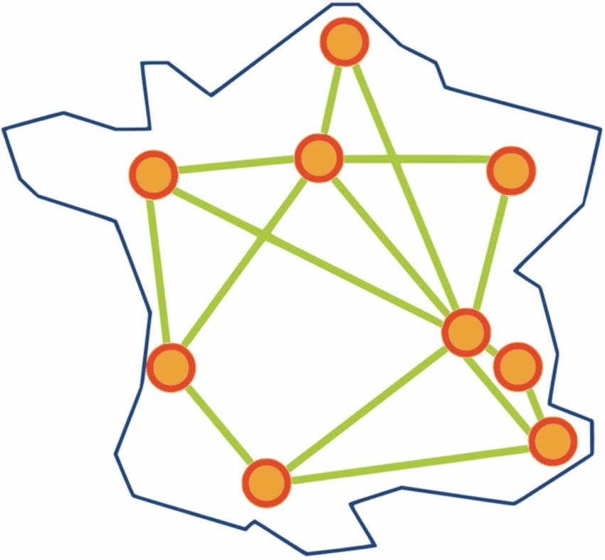
(a) Communications performance on Grid’5000 (b) Grid’5000: a nation-wide experimental testbed.
Fig. 3. Grid’5000 communication characteristics.
ScaLAPACK, and many of the linear algebra libraries for scientific computing, are programmed in
MPI. MPI is fit for homogeneous supercomputers: processes are mostly indistinguishable one from
another, and the standard does not specify anything about process / node placement.
As a consequence, to efficiently program a parallel application on top of a non-uniform network,
typically on top of a hierarchical network like a grid, MPI must be extended to help programmers adapt
the communications of the application to the machine. MPICH-G2 [29] introduced the concept of colors
to describe the available topology to the application at runtime. Colors can be used directly by MPI
routines in order to build topology-aware communicators (the abstraction in MPI that is used to group
processors together). However, the application is fully responsible to adapt itself to the topology that is
discovered at runtime. This adaptation, and the load-balancing that it implies, may be a hard task for
the application.
The QosCosGrid system8 offers a resource-aware grid meta-scheduler that gives the possibility to allo-
cate resources that match requirements expressed in a companion file called the application’s JobProfile
that describe the future communications of the application [6]. The JobProfile defines process groups
and requirements on the hardware specifications of the resources that have to be allocated for these
processes such as amount of memory, CPU speed, and network properties between groups of processes,
such as latency and bandwidth.
As a consequence, the application will always be executed on an appropriate resource topology. It
can therefore be developed for a specific topology in mind, for example, under the assumption that a
set of processes will be located on the same cluster or on the same multi-core machine. Of course, the
more flexibility the programmer gives to the JobProfile and the application, the more chances he gets
to let the meta-scheduler find a suitable hardware setup.
The QosCosGrid system features QCG-OMPI, an MPI implementation based on OpenMPI [21] and
targeted to computational grids. Besides grid-specific communication features that enable communicating
throughout the grid described in [15], QCG-OMPI has the possibility to retrieve topology information
provided to the scheduler in the JobProfile at run-time. We explain in Section III how we have
implemented and articulated TSQR with QCG-OMPI in order to take advantage of the topology.
8
Quasi-Opportunistic Supercomputing for Complex Systems in Grid Environments, http://www.qoscosgrid.euE. Scope
The QR factorization of TS matrices is directly used as a kernel in several important applications of
linear algebra. For instance, block-iterative methods need to regularly perform this operation in order to
obtain an orthogonal basis for a set of vectors; this step is of particular importance for block eigensolvers
(BLOPEX, SLEPc, PRIMME). Currently these packages rely on unstable orthogonalization schemes to
avoid too many communications. TSQR is a stable algorithm that enables the same total number of
messages. TSQR can also be used to perform the panel factorization of an algorithm handling general
matrices (CAQR). Thanks to simulations, Demmel et al. [17] anticipated that the benefits obtained with
TSQR should get transposed to CAQR. Said differently, this present study can be viewed as a first step
towards the factorization of general matrices on the grid.
Grids aggregate computing power from any kind of resource. However, in some typical grid projects,
such as Superlink@Technion, the Lattice project, EdGES, and the Condor pool at Univ. of Wisconsin-
Madison, a significant part of the power comes from a few institutions featuring environments with a
cluster-like setup. In this first work, we focus our study on clusters of clusters, to enable evaluation in a
stable and reproducible environment. Porting the work to a general desktop grid remains a future work.
Finally, we emphasize that the objective of this paper is to show that we can achieve a performance
speed up over the grid with common dense linear algebra operations. To illustrate our claim, we compare
our approach against a state-of-the-art library for distributed memory architectures, ScaLAPACK. In
order to highlight the differences, we chose to base our approach on ScaLAPACK (see Section III).
III. QCG-TSQR: A RTICULATION OF TSQR WITH QCG-OMPI
We explain in this section how we articulate the TSQR algorithm with QCG-OMPI in order to confine
intensive communications within the different geographical sites of the computational grid. The first
difference from the TSQR algorithm as presented in Section II-C is that a domain is processed by a
call to ScaLAPACK (but not LAPACK as in [17]). By doing so, we may attribute a domain to a group
of processes (instead of a single process) jointly performing its factorization. The particular case of
one domain per process corresponds to the original TSQR (calls to LAPACK). At the other end of the
spectrum, we may associate one domain per geographical site of the computational grid. The choice
of the number of domains impacts performance, as we will illustrate in Section V-D. In all cases, we
call our algorithm TSQR (or QCG-TSQR), since it is a single reduce operation based on a binary tree,
similarly to the algorithm presented in Section II-C.
As explained in Section II-D, the first task of developing a QCG-OMPI application consists of defining
the kind of topologies expected by the application in a JobProfile. To get enough flexibility, we request
that processes are split into groups of equivalent computing power, with good network connectivity
inside each group (low latency, high bandwidth) and we accept a lower network connectivity between
the groups. This corresponds to the classical cluster of clusters approach, with a constraint on the relative
size of the clusters to facilitate load balancing.
The meta-scheduler will allocate resources in the physical grid that matches these requirements. To
enable us to complete an exhaustive study on the different kind of topologies we can get, we also
introduced more constraints in the reservation mechanism, depending on the experiment we ran. For
each experiment, the set of machines that are allocated to the job are passed to the MPI middleware,
which exposes those groups using two-dimensional arrays of group identifiers (the group identifiers are
defined in the JobProfile by the developer). After the initialization, the application retrieves these group
identifiers from the system (using a specific MPI attribute) and then creates one MPI communicator per
group, using the MPI Comm split routine. Once this is done, the TSQR algorithm has knowledge of
the topology that allows it to adapt to the physical setup of the grid.
The choice to introduce a requirement of similar computing power between the groups however
introduces constraints on the reservation mechanism. For example, in some experiments discussed later
(Section V), only half the cores of some of the machines were allocated in order to fit this requirement.# msg vol. data exchanged # FLOPs
ScaLAPACK QR2 2N log2 (P ) log2 (P )(N 2 /2) (2M N 2 − 2/3N 3 )/P
TSQR log2 (P ) log2 (P )(N 2 /2) (2M N 2 − 2/3N 3 )/P + 2/3 log2 (P)N3
TABLE I
C OMMUNICATION AND COMPUTATION BREAKDOWN WHEN ONLY THE R- FACTOR IS NEEDED .
Another possibility would have been to handle load balancing issues at the algorithmic level (and not
at the middleware level) in order to relieve this constraint on the JobProfile and thus increase the
number of physical setups that would match our needs. In the particular case of TSQR, this is a natural
extension; we would only have to adapt the number of rows attributed to each domain as a function of
the processing power dedicated to a domain. This alternative approach is future work.
IV. P ERFORMANCE MODEL
In Tables I and II, we give the amount of communication and computation required for ScaLAPACK
QR2 and TSQR in two different scenarios: first, when only the R-factor is requested (Table I) and,
second, when both the R-factor and the Q-factor are requested (Table II). In this model, we assume that
a binary tree is used for the reductions and a homegeneous network. We recall that the input matrix A
is M –by–N and that P is the number of domains. The number of FLOPS is the number of FLOPS on
the critical path per domain.
Assuming a homogeneous network, the total time of the factorization is then approximated by the
formula:
time = β ∗ (# msg) + α ∗ (vol. data exchanged) + γ ∗ (# FLOPs) , (1)
where α is the inverse of the bandwidth, β the latency, and γ the inverse of the floating point rate of
a domain. Although this model is simplistic, it enables us to forecast the basic trends. Note that in the
case of TS matrices, we have M ≫ N .
First we observe that the cost to compute both the Q and the R factors is exactly twice the cost for
computing R only. Moreover, further theoretical and experimental analysis of the algorithm (see [17])
reveal that the structure of the computation is the same in both cases and the time to obtain Q is
twice the time to obtain R. This leads to Property 1. For brevity, we mainly focus our study on the
computation of R only.
Property 1: The time to compute both Q and R is about twice the cost for computing R only.
One of the building blocks of the ScaLAPACK PDGEQR2 implementation and of our TSQR algorithm
is the domanial QR factorization of a TS matrix. The domain can be processed by a core, a node or
a group of nodes. We can not expect performance from our parallel distributed algorithms to be better
than the one of its domanial kernels. This leads to Property 2. In practice, the performance of the
QR factorization of TS matrices obtained from LAPACK/ScaLAPACK on a domain (core, node, small
number of nodes) is a small fraction of the peak. (Term γ of Equation 1 is likely to be small.)
Property 2: The performance of the factorization of TS matrices is limited by the domanial perfor-
mance of the QR factorization of TS matrices.
We see that the number of operations is proportional to m while all the communication terms (latency
and bandwidth) are independent of m. Therefore when m increases, the communication time stays
constant whereas the domanial computation time increases. This leads to increased performance.
Property 3: The performance of the factorization of TS matrices increases with M .
The number of operations is proportional to N 2 while the number of messages is proportional to N .
Therefore when N increases, the latency term is hidden by the computation term. This leads to better
performance. We also note that increasing N enables better performance of the domanial kernel since
it can use Level 3 BLAS when the number of columns is greater than, perhaps, 100. This is Property 4.
Property 4: The performance of the factorization of TS matrices increases with N .
Finally, we see that the latency term is 2 log2 (P ) for TSQR while it is 2N log2 (P ) for ScaLAPACK
QR2. On the other hand, the FLOPs term has a non parallelizable additional 2/3 log2 (P)N3 term for# msg vol. data exchanged # FLOPs
ScaLAPACK QR2 4N log2 (P ) 2 log2 (P )(N 2 /2) (4M N 2 − 4/3N 3 )/P
TSQR 2 log2 (P ) 2 log2 (P )(N 2 /2) (4M N 2 − 4/3N 3 )/P + 4/3 log2 (P)N3
TABLE II
C OMMUNICATION AND COMPUTATION BREAKDOWN WHEN BOTH THE Q- FACTOR AND THE R- FACTOR ARE NEEDED .
the TSQR algorithm. We see that TSQR effectively trades messages for flops. We expect TSQR to be
faster than ScaLAPACK QR2 for N in the mid-range (perhaps between five and a few hundreds). For
larger N , TSQR will become slower because of the additional flops. This is Property 5. (We note that
for large N , one should stop using TSQR and switch to CAQR.)
Property 5: The performance of TSQR is better than ScaLAPACK for N in the mid range. When
N gets too large, the performance of TSQR deteriorates and ScaLAPACK becomes better.
V. E XPERIMENTAL STUDY
A. Experimental environment
We present an experimental study of the performance of the QR factorization of TS matrices in a
grid computing environment. We conducted our experiments on Grid’5000. This platform is a dedicated,
reconfigurable and controllable experimental grid of 13 clusters distributed over 9 cities in France. Each
cluster is itself composed of 58 to 342 nodes. The clusters are inter-connected through dedicated black
fiber. In total, Grid’5000 roughly gathers 5, 000 CPU cores featuring multiple architectures.
For the experiments presented in this study, we chose four clusters based on relatively homogeneous
dual-processor nodes, ranging from AMD Opteron 246 (2 GHz/1MB L2 cache) for the slowest ones
to AMD Opteron 2218 (2.6 GHz/2MB L2 cache) for the fastest ones, which leads to theoretical peaks
ranging from 8.0 to 10.4 Gflop/s per processor. These four clusters are the 93-node cluster in Bordeaux,
the 312-node cluster in Orsay, a 80-node cluster in Toulouse, and a 56-node cluster in Sophia-Antipolis.
Because these clusters are located in different cities, we will indistinctly use the terms cluster and
geographical site (or site) in the following. Nodes are interconnected with a Gigabit Ethernet switch;
on each node, the network controller is shared by both processors. On each cluster, we reserved a
subset of 32 dual-processor nodes, leading to a theoretical peak of 512.0 to 665.6 Gflop/s per node. Our
algorithm being synchronous, to evaluate the proportion of theoretical peak achieved in an heterogeneous
environment, we consider the efficiency of the slowest component as a base for the evaluation. Therefore,
the theoretical peak of our grid is equal to 2, 048 Gflop/s. A consequence of the constraints on the
topology expressed by our implementation in QCG-OMPI (see Section II-D) is that in some experiments,
machines with dual 2-cores processors were booked with the ability to use 2 cores (over 4) only.
The performance of the inter and intra-cluster communications is shown in Table 3(a). Within a
cluster, nodes are connected with a GigaEthernet network. Clusters are interconnected with 10 Gb/s
dark fibers. The intra-cluster throughput is consistently equal to 890 Mb/s but varies from 61 to 860
Mb/s between clusters. Inter-cluster latency is roughly greater than intra-cluster latency by two orders
of magnitude. Between two processors of a same node, OpenMPI uses a driver optimized for shared-
memory architectures, leading to a 17 µs latency and a 5 Gb/s throughput.
One major feature of the Grid5000 project is the ability of the user to boot her own environment
(including the operating system, distribution, libraries, etc.) on all the computing nodes booked for her
job. All the nodes were booted under Linux 2.6.30. The tests and benchmarks were compiled with GCC
4.0.3 (flag -O3) and run in dedicated mode (no other user can access the machines). ScaLAPACK 1.8.0
and GotoBLAS 1.26 libraries were used. Finally we recall that we focus on the factorization of TS
dense large-scale matrices in real double precision, corresponding to up to 16 GB of memory (e.g. a
33, 554, 432 × 64 matrix in double precision).B. Tuning of the applications To achieve high performance across platforms, dense linear algebra applications rely on Basic Linear Algebra Subprograms (BLAS) [13] to perform basic operations such as vector and matrix multiplication. This design by layers allows one to only focus on the optimization of these basic operations while keeping underlying numerical algorithms common to all machines. From the performance of BLAS operations – and in particular the matrix multiplication (DGEMM) – thus depends the behavior of the overall application. The Automatically Tuned Linear Algebra Software (ATLAS) [42] library is, for instance, a widely used implementation of BLAS achieving high performance thanks to autotuning methods. It is furthermore possible to take advantage of dual-processor nodes thanks to a multi-threaded implementation of BLAS such as GotoBLAS [24]. We have compared the performance of serial and multi-threaded GotoBLAS DGEMM against ATLAS. Both configurations of GotoBLAS outperformed ATLAS; we thus selected GotoBLAS to conduct our experiments. Another possibility to take advantage of dual-processor nodes is simply to create two processes per node at the application level. For both ScaLAPACK and TSQR, that latter configuration consistently achieved a higher performance. We therefore used two processes per node together with the serial version of GotoBLAS’s DGEMM in all the experiments reported in this study. With DGEMM being the fastest kernel (on top of which other BLAS operations are usually built), we obtain a rough practical performance upper bound for our computational grid of about 940 Gflop/s (the ideal case where 256 processors would achieve the performance of DGEMM, i.e., about 3.67 Gflop/s each) out of the 2, 048 Gflop/s theoretical peak. SCALAPACK implements block-partitioned algorithms. Its performance depends on the partitioning of the matrix into blocks. Preliminary experiments (not reported here) showed that a column-wise 1D- cyclic partition is optimum for processing TS matrices in our environment. We furthermore chose a block size consistently equal to 64 (a better tuning of this parameter as a function of the matrix characteristics would have occasionally improved the performance but we considered that the possible gain was not worth the degree of complexity introduced in the analysis of the results.). C. ScaLAPACK performance Figure 4 reports ScaLAPACK performance. In accordance with Property 2, the overall performance of the QR factorization of TS matrices is low (consistently lower than 90 Gflop/s) compared to the practical upper bound of our grid (940 Gflop/s). Even on a single cluster, this ratio is low since the performance at one site is consistently lower than 70 Gflop/s out of a practical upper bound of 235 Gflop/s. As expected too (properties 3 and 4), the performance increases with the dimensions of the matrix. For matrices of small to moderate height (M ≤ 5, 000, 000), the fastest execution is consistently the one conducted on a single site. In other words, for those matrices, the use of a grid (two or four sites) induces a drop in performance, confirming previous studies [34], [33], [41]. For very tall matrices (M > 5, 000, 000), the proportion of computation relative to the amount of communication becomes high enough so that the use of multiple sites eventually speeds up the performance (right-most part of the graphs and Property 3). This speed up however hardly surpasses a value of 2.0 while using four sites (Figure 4(b)). D. QCG-TSQR performance The performance of TSQR (articulated with QCG-OMPI as described in Section III) depends on the number of domains used. In Figure 5, we report the TSQR performance for the optimum number of domains and we will return later to the effect of the number of domains. In accordance with Property 2, the overall performance is again only a fraction of the practical upper bound of our grid (940 Gflop/s). But, compared to ScaLAPACK, this ratio is significantly higher since the factorization of a 8, 388, 608× 512 matrix achieves 256 Gflop/s (Figure 5(d)). Again, in accordance with properties 3 and 4, the overall performance increases with the dimensions of the matrix. Thanks to its better performance (Property 5), TSQR also achieves a speed up on the grid on matrices of moderate size. Indeed, for almost all matrices of moderate to great height (M ≥ 500, 000), the fastest execution is the one conducted on all four sites.
35                                                              60
                4 sites (128 nodes)                                             4 sites (128 nodes)
          30     2 sites (64 nodes)                                              2 sites (64 nodes)
                  1 site (32 nodes)                                       50
                                                                                  1 site (32 nodes)
          25
                                                                          40
Gflop/s

                                                                Gflop/s
          20
                                                                          30
          15
          10                                                              20

           5                                                              10

           0                                                               0
          100000         1e+06           1e+07          1e+08             100000         1e+06         1e+07      1e+08
                        Number of rows (M)                                              Number of rows (M)
                         (a) N = 64                                                     (b) N = 128

          60                                                              90
                4 sites (128 nodes)                                           4 sites (128 nodes)
          50     2 sites (64 nodes)                                       80   2 sites (64 nodes)
                  1 site (32 nodes)                                       70    1 site (32 nodes)
          40                                                              60
Gflop/s

                                                                Gflop/s
                                                                          50
          30
                                                                          40
          20                                                              30
                                                                          20
          10
                                                                          10
           0                                                               0
          100000                 1e+06                  1e+07             100000              1e+06               1e+07
                        Number of rows (M)                                              Number of rows (M)
                        (c) N = 256                                                     (d) N = 512

                                           Fig. 4.   ScaLAPACK performance.

          100                                                             140
              4 sites (128 nodes)                                                4 sites (128 nodes)
               2 sites (64 nodes)                                         120     2 sites (64 nodes)
           80   1 site (32 nodes)                                                  1 site (32 nodes)
                                                                          100
Gflop/s

                                                                Gflop/s

           60                                                              80

           40                                                              60
                                                                           40
           20
                                                                           20
            0                                                               0
           100000         1e+06           1e+07         1e+08              100000         1e+06           1e+07   1e+08
                        Number of rows (M)                                               Number of rows (M)
                        (a) N = 64                                                       (b) N = 128

          180                                                             300
                                                                                 4 sites (128 nodes)
          160 4 sites (128 nodes)                                                 2 sites (64 nodes)
               2 sites (64 nodes)                                         250
          140   1 site (32 nodes)                                                  1 site (32 nodes)
                                                                          200
          120
Gflop/s

                                                                Gflop/s

          100                                                             150
           80
                                                                          100
           60
                                                                           50
           40
           20                                                               0
           100000                 1e+06                 1e+07              100000                 1e+06           1e+07
                        Number of rows (M)                                               Number of rows (M)
                        (c) N = 256                                                      (d) N = 512

                                              Fig. 5.    TSQR Performance.
Furthermore, for very tall matrices (M ≥ 5, 000, 000), TSQR performance scales almost linearly with
the number of sites (a speed up of almost 4.0 is obtained on four sites). This result is the central
statement of this paper and validates the thesis that computational grids are a valid infrastructure for
solving large-scale problems relying on the QR factorization of TS matrices.
Figure 6 now illustrates the effect of the number of domains per cluster on TSQR performance.
Globally, the performance increases with the number of domains. For very tall matrices (M =
160
100 M = 33 554 432 M = 33 554 432
M = 4 194 304 140 M = 4 194 304
M = 524 288 120 M = 524 288
80 M = 131 072 M = 262 144
100
Gflop/s
Gflop/s
60
80
40 60
40
20
20
0 0
1 2 4 8 16 32 64 1 2 4 8 16 32 64
Number of domains per cluster Number of domains per cluster
(a) N = 64 (b) N = 128
250
M = 8 388 608 350 M = 8 388 608
M = 2 097 152 M = 2 097 152
200 M = 524 288 300 M = 524 288
M = 262 144 250 M = 262 144
Gflop/s
Gflop/s
150
200
100 150
100
50
50
0 0
1 2 4 8 16 32 64 1 2 4 8 16 32 64
Number of domains per cluster Number of domains per cluster
(c) N = 256 (d) N = 512
Fig. 6. Effect of the number of domains on the performance of TSQR executed on all four sites.
40 100
M = 8 388 608 M = 2 097 152
35 M = 1 048 576 M = 1 048 576
80 M = 131 072
30 M = 131 072 M = 65 536
25 M = 65 536
Gflop/s
Gflop/s
60
20
15 40
10
20
5
0 0
1 2 4 8 16 32 64 1 2 4 8 16 32 64
Number of domains Number of domains
(a) N = 64 (b) N = 512
Fig. 7. Effect of the number of domains on the performance of TSQR executed on a single site.
33, 554, 432), the impact is limited (but not negligible) since there is enough computation to almost
mask the effect of communications (Property 3). For very skinny matrices (N = 64), the optimum
number of domains for executing TSQR on a single cluster is 64 (Figure 7(a)), corresponding to a
configuration with one domain per processor. This optimum selection of the number of domains is
translated to executions on multiple clusters where 64 domains per cluster is optimum too (Figure 6(a)).
For the widest matrices studied (N = 512), the optimum number of domains for executing TSQR
on a single cluster is 32 (Figure 7(b)), corresponding to a configuration with one domain per node.For those matrices, trading flops for intra-node communications is not worthwhile. This behavior is
again transposable to executions on multiple sites (Figure 6(d)) where the optimum configuration also
corresponds to 32 domains per cluster. This observation illustrates the fact that one should use CAQR
and not TSQR for large N , as discussed in Section IV.
E. QCG-TSQR vs ScaLAPACK
Figure 8 compares TSQR performance (still articulated with QCG-OMPI) against ScaLAPACK’s. We
90 TSQR (best) 120 TSQR (best)
80 ScaLAPACK (best) ScaLAPACK (best)
70 100
60 80
Gflop/s
Gflop/s
50
60
40
30 40
20
20
10
0 0
100000 1e+06 1e+07 1e+08 100000 1e+06 1e+07 1e+08
Number of rows (M) Number of rows (M)
(a) N = 64 (b) N = 128
180 300
160 TSQR (best) Gflop/s 250 TSQR (best)
ScaLAPACK (best) ScaLAPACK (best)
140
200
120
Gflop/s
100 150
80 100
60
50
40
20 0
100000 1e+06 1e+07 100000 1e+06 1e+07
Number of rows (M) Number of rows (M)
(c) N = 256 (d) N = 512
Fig. 8. TSQR vs ScaLAPACK. For each algorithm, the performance of the optimum configuration (one, two or four sites) is reported.
report the maximum performance out of executions on one, two or four sites. For instance, the graph
of TSQR in Figure 8(a) is thus the convex hull of the three graphs from Figure 5(a). In accordance
with Property 5, TSQR consistently achieves a higher performance than ScaLAPACK. For matrices of
limited height (M = 131, 072), TSQR is optimum when executed on one site (Figure 5(a)). In this
case, its superiority over ScaLAPACK comes from better performance within a cluster (Figure 7(a)).
For matrices with a larger number of rows (M = 4, 194, 304), the impact of the number of domains per
cluster is less sensitive (Figure 7(a) and Property 3). On the other hand, the matrix is large enough to
allow a speed up of TSQR over the grid (Figure 5(a) and Property 3 (again)) but not of ScaLAPACK
(Figure 4(a) and Property 5), hence the superiority of TSQR over ScaLAPACK for that type of matrix.
For very tall matrices (M = 33, 554, 432), the impact of the number of domains per cluster becomes
negligible (Figure 7(a) and Property 3). But (i) TSQR achieves a speed up of almost 4.0 on four sites
(Figure 5(a)) whereas (ii) ScaLAPACK does not achieve yet such an ideal speed up (Figure 4(a)).
Finally, on all the range of matrix shapes considered, and for different reasons, we have seen that
TSQR consistently achieves a significantly higher performance than ScaLAPACK. For not so tall and
not so skinny matrices (left-most part of Figure 8(d)), the gap between the performance of TSQR and
ScaLAPACK reduces (Property 5).
One may have observed that the time spent in intra-node, then intra-cluster and finally inter-cluster
communications becomes negligible while the dimensions of the matrices increase. For larger matrices
(which would not hold in the memory of our machines), we may thus even expect that communicationsover the grid for ScaLAPACK would become negligible and thus that TSQR and ScaLAPACK would
eventually achieve a similar (scalable) performance (Property 5).
VI. C ONCLUSION AND PERSPECTIVES
This paper has revisited the performance behavior of common dense linear algebra operations in
a grid computing environment. Contrary to past studies, we have shown that they can achieve a
performance speed up by using multiple geographical sites of a computational grid. To do so, we have
articulated a recently proposed algorithm (CAQR) with a topology-aware middleware (QCG-OMPI) in
order to confine intensive communications (ScaLAPACK calls) within the different geographical sites.
Our experimental study, conducted on the experimental Grid’5000 platform, focused on a particular
operation, the QR factorization of TS matrices. We showed that its performance increases linearly with
the number of geographical sites on large-scale problems (and is in particular consistently higher than
ScaLAPACK’s).
We have proved theoretically through our models and experimentally that TSQR is a scalable al-
gorithm on the grid. TSQR is an important algorithm in itself since, given a set of vectors, TSQR is
a stable way to generate an orthogonal basis for it. TSQR will come handy as an orthogonalization
scheme for sparse iterative methods (eigensolvers or linear solves). TSQR is also the panel factorization
of CAQR. A natural question is whether CAQR scales as well on the grid. From models, there is no
doubt that CAQR should scale. However we will need to perform the experiment to confirm this claim.
We note that the work and conclusion we have reached here for TSQR/CAQR can be (trivially) extended
to TSLU/CALU ([25]) and Cholesky factorization [5].
Our approach is based on ScaLAPACK. However, recent algorithms that better fit emerging archi-
tectures would have certainly improved the performance obtained on each cluster and in fine the global
performance. For instance, recursive factorizations have been shown to achieve a higher performance
on distributed memory machines [17]. Other codes benefit from multicore architectures [1].
If, as discussed in the introduction, the barriers for computational grids to compete against supercom-
puters are multiple, this study shows that the performance of large-scale dense linear algebra applications
can scale with the number of geographical sites. We plan to extend this work to the QR factorization of
general matrices and then to other one-sided factorizations (Cholesky, LU). Load balancing to take into
account heterogeneity of clusters is another direction to investigate. The use of recursive algorithms to
achieve higher performance is to be studied too.
T HANKS
The authors thank Laura Grigori for her constructive suggestions.
R EFERENCES
[1] E. Agullo, B. Hadri, H. Ltaief, and J. Dongarra. Comparative study of one-sided factorizations with multiple software packages on
multi-core hardware. In SC, 2009.
[2] Bruce Allen, Carl Christensen, Neil Massey, Tolu Aina, and Miguel Angel Marquina. Network computing with einstein@home and
climateprediction.net. Technical report, CERN, Geneva, Jul 2005. CERN, Geneva, 11 Jul 2005.
[3] David P. Anderson. BOINC: A system for public-resource computing and storage. In Rajkumar Buyya, editor, GRID, pages 4–10.
IEEE Computer Society, 2004.
[4] R. M. Badia, D. Du, E. Huedo, A. Kokossis, I. M. Llorente, R. S. Montero, M. de Palol, R. Sirvent, and C. Vázquez. Integration of
GRID superscalar and gridway metascheduler with the DRMAA OGF standard. In Proceedings of the 14th International Euro-Par
Conference, volume 5168 of LNCS, pages 445–455. Springer, 2008.
[5] Grey Ballard, James Demmel, Olga Holtz, and Oded Schwartz. Communication-optimal parallel and sequential Cholesky
decomposition: extended abstract. In SPAA, pages 245–252, 2009.
[6] P Bar, C Coti, D Groen, T Herault, V Kravtsov, A Schuster, and Running parallel applications with topology-aware grid middleware.
In 5th IEEE International Conference on e-Science (eScience’09), December 2009. to appear.
[7] A L. Beberg, D L. Ensign, G Jayachandran, S Khaliq, and V S. Pande. Folding@home: Lessons from eight years of volunteer
distributed computing. In 8th IEEE International Workshop on High Performance Computational Biology (HiCOMB 2009).
[8] L. S. Blackford, J. Choi, A. Cleary, E. D’Azevedo, J. Demmel, I. Dhillon, J. Dongarra, S. Hammarling, G. Henry, A. Petitet,
K. Stanley, D. Walker, and R. Whaley. ScaLAPACK Users’ Guide. SIAM, 1997.[9] Raphaël Bolze. Analyse et déploiement de solutions algorithmiques et logicielles pour des applications bioinformatiques à grande
échelle sur la grille. PhD thesis, École Normale Supérieure de Lyon, October 2008.
[10] Alfredo Buttari, Julien Langou, Jakub Kurzak, and Jack Dongarra. A class of parallel tiled linear algebra algorithms for multicore
architectures. Parallel Computing, 35:38–53, 2009.
[11] E Caron, F Desprez, and C Tedeschi. Efficiency of tree-structured peer-to-peer service discovery systems. In IPDPS, pages 1–8,
2008.
[12] J Choi, J Demmel, I S. Dhillon, J Dongarra, S Ostrouchov, A Petitet, K Stanley, D W. Walker, and R. C Whaley. ScaLAPACK: A
portable linear algebra library for distributed memory computers - design issues and performance. In PARA, pages 95–106, 1995.
[13] Jaeyoung Choi, Jack Dongarra, Susan Ostrouchov, Antoine Petitet, David W. Walker, and R. Clinton Whaley. A proposal for a set
of parallel basic linear algebra subprograms. In PARA, pages 107–114, 1995.
[14] E. Chu and A. George. QR factorization of a dense matrix on a hypercube multiprocessor. SIAM J. Sci. Stat. Comput., 11(5):990–
1028, 1990.
[15] C Coti, T Herault, S Peyronnet, A Rezmerita, and F Cappello. Grid services for MPI. In ACM/IEEE, editor, Proceedings of the
8th IEEE International Symposium on Cluster Computing and the Grid (CCGrid’08), pages 417–424, Lyon, France, May 2008.
[16] R Das, B Qian, S Raman, R Vernon, J Thompson, P Bradley, S Khare, M D D. Tyka, D Bhat, D Chivian, David E E. K, W H H.
Sheffler, L Malmström, A M M. Wollacott, C Wang, I Andre, and D Baker. Structure prediction for CASP7 targets using extensive
all-atom refinement with rosetta@home. Proteins, 69(S8):118–128, September 2007.
[17] J Demmel, L Grigori, M Hoemmen, and J Langou. Communication-avoiding parallel and sequential QR factorizations. CoRR,
arixv.org/abs/0806.2159, 2008.
[18] Jack Dongarra, Piotr Luszczek, and Antoine Petitet. The LINPACK benchmark: past, present and future. Concurrency and
Computation: Practice and Experience, 15(9):803–820, 2003.
[19] Message Passing Interface Forum. MPI: A message-passing interface standard. Technical Report UT-CS-94-230, Department of
Computer Science, University of Tennessee, April 1994.
[20] I Foster and C Kesselman. The Grid: Blueprint for a New Computing Infrastructure. Morgan Kaufmann Publishers, 2 edition, 2003.
[21] E Gabriel, G E. Fagg, G Bosilca, T Angskun, J J. Dongarra, J M. Squyres, V Sahay, P Kambadur, B Barrett, A Lumsdaine,
R H. Castain, D J. Daniel, R L. Graham, and T S. Woodall. Open MPI: Goals, concept, and design of a next generation MPI
implementation. In Proceedings, 11th European PVM/MPI Users’ Group Meeting, pages 97–104, Budapest, Hungary, September
2004.
[22] E Gabriel, M M. Resch, T Beisel, and R Keller. Distributed computing in a heterogeneous computing environment. In Proceedings
of the 5th European PVM/MPI Users’ Group Meeting, volume 1497 of LNCS, pages 180–187. Springer, 1998.
[23] G. H. Golub and C. F. Van Loan. Matrix Computations. Johns Hopkins University Press, Baltimore, USA, 2 edition, 1989.
[24] K Goto and R A. van de Geijn. High-performance implementation of the level-3 blas. ACM Trans. Math. Softw., 35(1), 2008.
[25] Laura Grigori, James Demmel, and Hua Xiang. Communication avoiding Gaussian elimination. In SC, page 29, 2008.
[26] B. C. Gunter and R. A. van de Geijn. Parallel out-of-core computation and updating of the QR factorization. ACM Trans. on Math.
Soft., 31(1):60–78, March 2005.
[27] D. Heller. A survey of parallel algorithms in numerical linear algebra. SIAM Rev., (20):740–777, 1978.
[28] Marty Humphrey, Mary Thompson, and Keith Jackson. Security for grids. IEEE, 3:644 – 652, March 2005.
[29] Nicholas T. Karonis, Brian R. Toonen, and Ian T. Foster. MPICH-G2: A grid-enabled implementation of the message passing
interface. CoRR, arxiv.org/cs.DC/0206040, 2002.
[30] J. Kurzak and J. J. Dongarra. QR factorization for the CELL processor. Scientific Programming, Special Issue: High Performance
Computing with the Cell Broadband Engine, 17(1-2):31–42, 2009.
[31] Stefan M. Larson, Christopher D. Snow, Michael Shirts, and Vijay S. Pande. Folding@home and genome@home: Using distributed
computing to tackle previously intractable problems in computational biology. (arxiv.org/abs/arxiv:0901.0866), 2009.
[32] R.E. Lord, J.S. Kowalik, and S.P. Kumar. Solving linear algebraic equations on an MIMD computer. J. ACM, 30(1):103–117, 1983.
[33] Jeff Napper and Paolo Bientinesi. Can cloud computing reach the Top500? Technical Report AICES-2009-5, Aachen Institute for
Computational Engineering Science, RWTH Aachen, February 2009.
[34] A Petitet, S Blackford, J Dongarra, B Ellis, G Fagg, K Roche, and S Vadhiyar. Numerical libraries and the grid: The GrADS
experiments with ScaLAPACK. Technical Report UT-CS-01-460, ICL, U. of Tennessee, April 2001.
[35] A. Pothen and P. Raghavan. Distributed orthogonal factorization: Givens and Householder algorithms. SIAM Journal on Scientific
and Statistical Computing, 10:1113–1134, 1989.
[36] G. Quintana-Ortı́, E. S. Quintana-Ortı́, E. Chan, F. G. Van Zee, and R. A. van de Geijn. Scheduling of QR factorization algorithms
on SMP and multi-core architectures. In Proceedings of PDP’08, 2008. FLAME Working Note #24.
[37] R. Reddy and A. Lastovetsky. HeteroMPI + ScaLAPACK: Towards a ScaLAPACK (Dense Linear Solvers) on heterogeneous networks
of computers. volume 4297, pages 242–253, Bangalore, India, 18-21 Dec 2006 2006. Springer, Springer.
[38] A. Sameh and D. Kuck. On stable parallel linear system solvers. J. ACM, 25(1):81–91, 1978.
[39] R. Schreiber and C. Van Loan. A storage efficient W Y representation for products of Householder transformations. SIAM J. Sci.
Stat. Comput., 10(1):53–57, 1989.
[40] Sathish S. Vadhiyar and Jack J. Dongarra. Self adaptivity in grid computing. Concurrency & Computation: Practice & Experience,
2005.
[41] Edward Walker. Benchmarking amazon EC2 for high-performance scientific computing. USENIX Login, 33(5):18–23, 2008.
[42] R. Clint Whaley, Antoine Petitet, and Jack J. Dongarra. Automated empirical optimization of software and the ATLAS project.
Parallel Comput., 27(1–2):3–25, 2001.You can also read