The interannual variability of Africa's ecosystem productivity: a multi-model analysis
←
→
Page content transcription
If your browser does not render page correctly, please read the page content below
Biogeosciences, 6, 285–295, 2009
www.biogeosciences.net/6/285/2009/                                                                  Biogeosciences
© Author(s) 2009. This work is distributed under
the Creative Commons Attribution 3.0 License.

The interannual variability of Africa’s ecosystem productivity: a
multi-model analysis
U. Weber1,2 , M. Jung2 , M. Reichstein2 , C. Beer2 , M. C. Braakhekke2 , V. Lehsten3 , D. Ghent4 , J. Kaduk4 , N. Viovy5 ,
P. Ciais5 , N. Gobron6 , and C. Rödenbeck2
1 Department  of Forest Science and Environment,University of Tuscia, Viterbo, Italy
2 Max Planck Institute for Biogeochemistry, Jena, Germany
3 GeoBiosphere Science Centre, Lund University, Sweden
4 Department of Geography, University of Leicester, UK
5 Laboratoire des Sciences du Climate et de l’ Environnement, Gif-sur-Yvette, France
6 European Commission – DG Joint Research Centre, Institute for Environment and Sustainability, Global Environment

Monitoring Unit, Ispra (VA), Italy
Received: 4 August 2008 – Published in Biogeosciences Discuss.: 10 October 2008
Revised: 2 February 2009 – Accepted: 17 February 2009 – Published: 25 February 2009

Abstract. We are comparing spatially explicit process-             estimates of surface carbon fluxes are less conclusive at this
model based estimates of the terrestrial carbon balance and        point, implying the need for a denser network of observation
its components over Africa and confront them with remote           stations over Africa.
sensing based proxies of vegetation productivity and atmo-
spheric inversions of land-atmosphere net carbon exchange.
Particular emphasis is on characterizing the patterns of inter-    1   Introduction
annual variability of carbon fluxes and analyzing the factors
and processes responsible for it. For this purpose simula-         Understanding terrestrial sources and sinks of CO2 and its
tions with the terrestrial biosphere models ORCHIDEE, LPJ-         variability is important for understanding the carbon cycle-
DGVM, LPJ-Guess and JULES have been performed using                climate feedback. Extensive research in this field has con-
a standardized modeling protocol and a uniform set of cor-         centrated on the highly developed parts of the world, in par-
rected climate forcing data.                                       ticular North America and Europe with a strong research in-
   While the models differ concerning the absolute magni-          frastructure. In a recent review, Williams et al. (2007) identi-
tude of carbon fluxes, we find several robust patterns of inter-   fied Africa as “one of the weakest links in our understanding
annual variability among the models. Models exhibit largest        of the global carbon cycle.” Africa is the second largest con-
interannual variability in southern and eastern Africa, regions    tinent of the world occupying about 20% of global land mass
which are primarily covered by herbaceous vegetation. In-          and inhabits a large variety of ecosystems ranging from per-
terannual variability of the net carbon balance appears to be      humid tropical forest to semi-arid and arid grass and shrub
more strongly influenced by gross primary production than          communities. Although Africa’s decadal scale mean carbon
by ecosystem respiration. A principal component analysis in-       balance appears to be neutral, the continent contributes about
dicates that moisture is the main driving factor of interannual    half of the interannual variability of the carbon balance on
gross primary production variability for those regions. On         global scale (Williams et al., 2007). This large interannual
the contrary in a large part of the inner tropics radiation ap-    variability results primarily from climatic perturbations re-
pears to be limiting in two models. These patterns are partly      lated to the El Nino phenomenon that directly affects the
corroborated by remotely sensed vegetation properties from         ecosystems’ productivity and due to concomitant biomass
the SeaWiFS satellite sensor. Inverse atmospheric modeling         burning (e.g. Le Page et al., 2007; Anyamba et al., 2002,
                                                                   2003; Myneni et al., 1996; Kogan 2000).
                                                                      Given the scarcity of observation sites for atmospheric
                     Correspondence to: U. Weber                   CO2 concentrations and land – atmosphere CO2 exchange
                     (uweber@bgc-jena.mpg.de)                      the uncertainties of African carbon cycle research remain

Published by Copernicus Publications on behalf of the European Geosciences Union.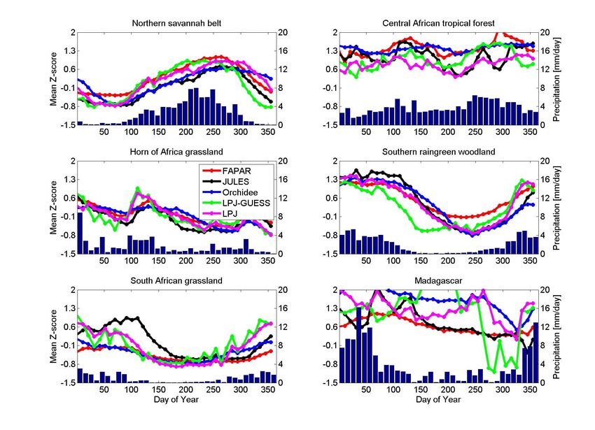
286                                                    U. Weber et al.: Interannual variability of Africas ecosystem productivity

high in particular regarding the spatial localization of hotspot   LPJ-DGVM and LPJ-GUESS are designed as stand-alone
regions of variability and the underlying driving forces. Sim-     models running on a daily time step, ORCHIDEE and
ulations of terrestrial ecosystem models can provide insights      JULES can be coupled to General Circulation Models func-
here; however, these models are also associated with large         tioning as land-surface schemes. Therefore, latter models re-
uncertainties (e.g. McGuire et al., 2001; Friedlingstein et al.,   solve the diurnal cycle with time steps of 30 to 60 min. Usu-
2006) in particular for water limited conditions (e.g. Morales     ally, the LPJ family of models is driven by monthly climatic
et al., 2005; Jung et al., 2007), and in addition have gener-      data which are interpolated to pseudo-daily using a whether
ally not been tested and parameterized specifically for Africa.    generator for precipitation. In this study, the LPJ-DGVM is
Thus, confidence of a single model analysis is limited and a       driven by daily climatic inputs. In doing so, net radiation
multi-model study is warranted to identify coherent and dis-       is approximated from global radiation after Linacre (1969).
similar behavior between different biosphere models.               The LPJ-GUESS has the most advanced representation of
   In this study we assess the interannual variability of          vegetation structure including age with features of a forest-
Africa’s carbon cycle using four different terrestrial carbon      gap model (Shugart, 1984) resolving forest succession. LPJ-
cycle models in conjunction with remotely sensed indicators        DGVM and ORCHIDEE have intermediate complexity ap-
for the state of the vegetation as well as carbon balance esti-    plying the concept of “average individuals” for a whole grid
mates from global atmospheric inversions. We aim to iden-          cell (Sitch et al., 2003) while JULES/TRIFFID employs a
tify (1) regions of largest carbon balance interannual variabil-   heuristic approach to determine the vegetation coverage and
ity, (2) the primary process (photosynthesis or respiration)       carbon allocation to each PFT.
dominating the carbon balance variability, and (3) which cli-
mate variables are driving the ecosystem’s carbon cycle in         2.2   Model drivers
the models.
                                                                   All models are driven by the same climate data, atmospheric
                                                                   CO2 concentration, and soil texture type on a 1◦ grid from
                                                                   1982 to 2006, which has been derived as follows: Meteo-
2     Materials and methods
                                                                   rological forcing (near surface air temperature, specific hu-
2.1    Model descriptions                                          midity, wind speed, radiation, and precipitation) originates
                                                                   from 6-hourly NCEP-DOE Reanalysis-2 (Kanamitsu et al.,
The four ecosystem models ORCHIDEE (Krinner et al.,                2002) that were spatially interpolated to 1◦ from the origi-
2005), LPJ-DGVM (Sitch et al., 2003), LPJ-GUESS (Smith             nal T62 Gaussian grid. Despite substantial improvements of
et al., 2001), and JULES/TRIFFID (Cox et al., 2001; Es-            NCEP R2 over R1 considerable precipitation biases remain
sery et al., 2001; Hughes et al., 2006) applied in this            in comparison to various independent data sets (Fekete et al.,
study are coupled biogeography-biogeochemistry models,             2004). To account for these limitations, precipitation was
i.e. they combine representations of both vegetation dynam-        corrected using more reliable data sets based on observations
ics and land-atmosphere carbon and water exchanges (dy-            from the satellite based Tropical Rainfall Measuring Mission
namic global vegetation models – DGVMs). The concept of            (TRMM 3B43) available from 1998–2006 (Kummerow et
plant functional types (PFT) (Smith et al., 1997) is used to       al., 1998) and from interpolated station data provided by the
discretize differences in physiology and allometry of species      Climate Research Unit (CRU) from 1961–2003 (CRUTR2.1,
including adaptations to climatic conditions and disturbance       Mitchell and Jones, 2005). The general calibration method
regime. PFTs compete for resources like light, and water.          follows Williams et al. (2008), Ngo-Duc et al. (2005) and
Representations of vegetation structure like allometry, and        Sheffield et al. (2006), where the daily values of the origi-
function like phenology, allocation, mortality, and establish-     nal NCEP data for each grid cell are scaled to match in their
ment are essential for this. Gross primary production (GPP)        monthly totals those of the corresponding CRU and TRMM
is calculated based on a coupled photosynthesis-water bal-         data. For the CRU period (1979–1997) precipitation was cor-
ance scheme after (Farquhar et al., 1980; Collatz et al., 1991,    rected following:
1992), where simplifications have been incorporated in the
different models as described in detail in the above refer-                              NCEPy,m,d,h × CRUy,m
ences. Heterotrophic respiration is assumed to be represented      CAl NCEPy,m,d,h =                          ×               (1)
                                                                                                NCEPy,m
by first-order decay of organic material with decay rates for                            P2006
a few pools (Foley, 1995) which depend on temperature and                                  1998 TRMMm
                                                                                          P2006
moisture following (Lloyd and Talor, 1994) or a Q10 formula.                                1998 CRUm
Fire, the main disturbance in the region is simulated follow-
                                                                      For the TRMM period (1998–2006) the calibration used:
ing (Thonicke et al., 2001) within LPJ-DGVM, ORCHIDEE,
and LPJ-GUESS.                                                                                           TRMMy,m
                                                                   CAl NCEPy,m,d,h = NCEPy,m,d,h ×                            (2)
   The applied models differ in the temporal resolution and in                                           NCEPy,m
the resolution of vegetation structure representations. While

Biogeosciences, 6, 285–295, 2009                                                           www.biogeosciences.net/6/285/2009/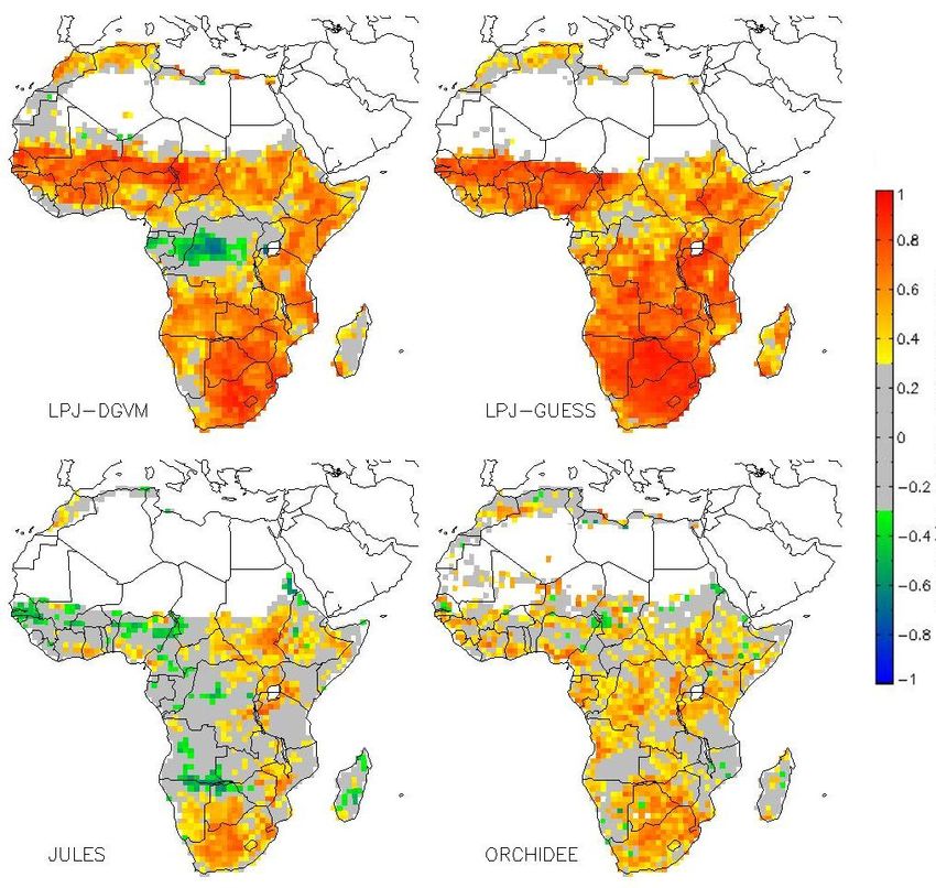
U. Weber et al.: Interannual variability of Africas ecosystem productivity                                                   287

                                                                  Quantification of interannual variability

                                                                     Interannual variability (IAV) is calculated for each pixel
                                                                  and model as the standard deviation of the respective quantity
                                                                  (e.g. GPP) for a yearly time step across all years, resulting in
                                                                  a grid of IAV for each model and variable. For identifying
                                                                  spatial patterns of relatively high and low interannual vari-
                                                                  ability, the IAV grid of each model was z-transformed.

                                                                                 IAVi − IAV
                                                                  z (IAVi ) =
                                                                                    σIAV

                                                                     Where z(IAVI ) is the standardized IAV of grid cell i, IAV
                                                                  and σIAV are the spatial mean and standard deviation of the
                                                                  IAV, respectively. Hence z(IAVI ) measures the degree of
                                                                  variability for each pixel in units of standard deviations, i.e.
                                                                  values larger than 0 refer to above average interannual vari-
                                                                  ability and for example a value of two indicates variability
                                                                  of 2 standard deviations above the mean variability of the
                                                                  continent. Consistent spatial patterns between all models
Fig. 1. African ecoregions                                        are defined as model agreement and are implemented as the
                                                                  sum of models per grid cell which show variability larger
                                                                  than one standard deviation above the mean variability of
   The adjustment yielded an overall reduction of 15.2% pre-      the continent.
cipitation.
   Soil texture is given by the IGBP-DIS map at 1◦ (Tempel et     Principal component analysis
al., 1996). Data on the annual CO2 concentration was taken
from measurements at Mauna Loa (www.esrl.noaa.gov/gmd/
                                                                     To analyze the relationship between meteorological
ccgg/trends/).
                                                                  conditions and simulated carbon fluxes on annual scale we
2.3   Experimental setup                                          follow the approach of Jung et al. (2007). First we reduce
                                                                  the array of several meteorological driver variables to their
The simulation of the terrestrial carbon and water budgets are    principal components and then calculate the correlation
carried out at a spatial resolution of 1◦ ×1◦ for entire conti-   between meteorological principal components and relative
nental Africa for the target period 1982–2006. Spin-up cal-       flux variations for each grid cell. The principal component
culations were performed by repeating the years 1982–1992         analysis (PCA) of the meteorological data reduces the
using the meteorological data sets of the appropriate years       dimensionality of the data set and often extracts major
and a fixed CO2 concentration of 341.13 ppm (Mauna Loa            weather patterns or gradients. We used four annual data
value in 1982) until carbon pools reach equilibrium. After        fields as input to the PCA: precipitation, air temperature,
the spin-up, model simulations start in 1982 with rising CO2      radiation, specific air humidity.
concentration per annum. Potential vegetation distribution
was dynamically simulated by the models.                          Corroboration against satellite data

2.4   Data analysis                                                  We use the fraction of absorbed photosynthetic active radi-
                                                                  ation (FAPAR) product of Gobron et al. (2006) based on the
Definition of regions                                             SeaWiFS satellite sensor as a proxy for vegetation productiv-
                                                                  ity (available at: www.fapar.jrc.it). It has been designed as an
   We define six major regions of sub-saharan Africa based        optimized indicator for the state and health of the vegetation
on the broad distribution of ecosystem types (available from      and overcomes several limitations of the classically used nor-
global land cover maps), and thus implicitly according            malized difference vegetation index (NDVI) (Gobron et al.,
to bioclimatic conditions: Northern Savannah Belt, Cen-           2000). Jung et al. (2008) have shown that the annual sum
tral African tropical forest, Horn of Africa, Southern rain-      of FAPAR growing season values correlates strongly with
green woodlands, South African grasslands, and Madagascar         annual gross primary production from eddy covariance mea-
(Fig. 1). Given that Madagascar is small in comparison to the     surement sites in Europe. At first glance it appears to be more
other regions and very heterogeneous we do not discuss this       consistent to compare simulated FAPAR by the models with
region extensively.                                               the FAPAR satellite retrievals instead of using the FAPAR as

www.biogeosciences.net/6/285/2009/                                                           Biogeosciences, 6, 285–295, 2009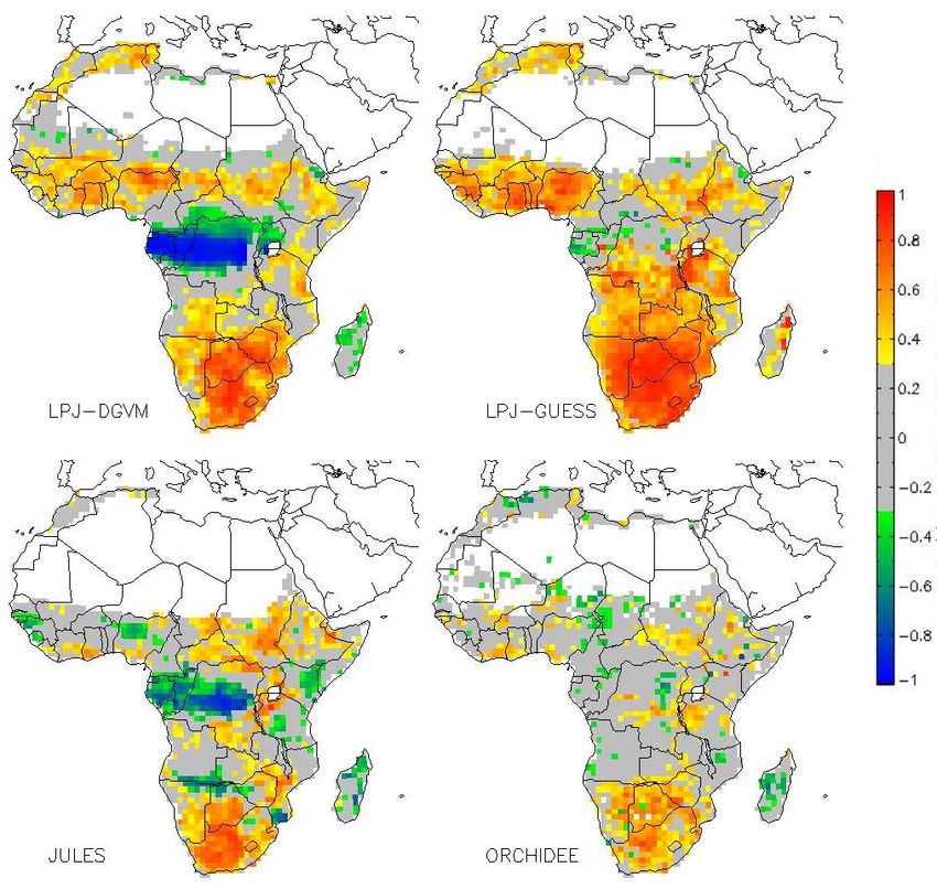
288                                                   U. Weber et al.: Interannual variability of Africas ecosystem productivity

a proxy for GPP. However, there are several reasons why it        Table 1. Continental annual average GPP, NPP per model (temporal
makes more sense to interpret the remotely sensed FAPAR as        standard deviation), all numbers are in Pg C y-1
an indicator for productivity: (1) ecosystem models tend to
capture interannual variability of GPP primarily via interan-               LPJ DGVM       LPJ GUESS      JULES          ORCHIDEE
nual variations of radiation use efficiency and not via changes
                                                                      GPP   39.68 [1.73]   16.58 [1.04]   31.50 [0.91]   29.80 [1.20]
of leaf area (Jung et al., 2007) while the interannual anomaly        NPP   17.28 [1.12]   9.16 [0.67]    12.01 [0.48]   15.38 [0.77]
patterns of the SeaWiFS-FAPAR provide a realistic picture of
the GPP anomalies (Jung et al., 2008; Gobron et al., 2005),
and (2) there are conceptual mismatches between the FAPAR
from the satellite and the FAPAR simulated by models. For         3     Results and discussion
example the response of herbaceous understorey, which is
very sensitive to e.g. water stress, plays likely an important    3.1    Mean annual carbon fluxes
role in the anomaly patterns of the satellite FAPAR by indi-
cating the direction of change of the ecosystem (see in Jung      We use annual sums of GPP and Net Primary Production
et al., 2008 for more discussion). In addition, changes of        (NPP) over the entire study period to investigate the mean
the remotely sensed FAPAR may originate from changes of           annual carbon fluxes at the continental as well as on the re-
leaf colour (e.g. leaf darkening or yellowing), which indi-       gional scale, and compare them to global numbers based on
cates changes of chlorophyll content and thus radiation use       the IPCC Fourth Assessment Report (IPCC 2007). Mod-
efficiency. In contrast, the leaves in the models do not change   elled absolute NEP estimates strongly depend on factors that
their reflective properties; effects of leaf aging on photosyn-   cannot be taken into account (e.g. change in land-use his-
thesis are in some cases captured as Vcmax being a function       tory) and thus are relatively meaningless. Hence, we dis-
of leaf age as in ORCHIDEE.                                       cuss NEP only in terms of interannual variability as previ-
   We calculate mean annual FAPAR as a proxy for GPP              ously done in other contexts (e.g., Ciais et al., 2005; Vet-
after filling gaps of the FAPAR time series as described          ter et al., 2008) (see below). At continental scale annual
in Jung et al. (2008). In addition we compare the mean            GPP estimates range from 16.58 to 39.68 Pg C y-1 (14–33%
seasonal cycles of simulated GPP and remotely sensed              of global GPP (120 Pg C y-1)), and 9.16 to 17.28 Pg C y-1
FAPAR for the defined regions.                                    for NPP (14–27% of global NPP (65 Pg C y-1)) respectively
                                                                  (Table 1). Previous modeling studies indicated mean annual
Comparison with atmospheric inversions                            NPP between 7 and 13 Pg C y-1 (Cramer et al., 1999; Cao et
                                                                  al., 2001; Potter, 2003). Possibly, the too extensive forest
   We compare the simulated variations of the African car-        cover simulated by LPJ-DGVM (17.28 Pg C y-1) and OR-
bon balance in terms of Net Ecosystem Productivity (NEP),         CHIDEE (15.38 Pg C y-1) may have caused an overestima-
and Net Biome Production (NBP) with results from global           tion of continental scale NPP. A realistic representation of
atmospheric inversions from Rödenbeck (2005) (version            savannah ecosystems is still a challenge for dynamic vegeta-
s96 v3.1) covering the period of 1997 to 2006 based on glob-      tion models.
ally 51 stations of atmospheric CO2 records. This way we             The comparison of simulated interannual variations of the
also determine the role of fire on the interannual variability    African carbon balance with atmospheric inversions reveals
of the carbon balance. Simulated NEP is calculated as GPP         a consistent pattern but some discrepancies remain (Fig. 2).
minus Terrestrial Ecosystem Respiration (TER). Modeled            There is agreement of above average net uptake for 1997,
NBP is based on the difference of NEP and model specific          2000, 2001, and 2006 and a below average carbon balance
fire emissions, except JULES which does not include fire.         for 1998, 2002, 2003 and 2005. The general pattern of conti-
The inversions detect carbon emissions from fire. To facili-      nental scale IAV is consistent between NEP and NBP, which
tate comparability between NEP simulations and inversions,        indicates a small contribution of fire emissions on the vari-
we used the Global Fire Emission Database (GFED version           ability of the African carbon balance in the considered pe-
2.1, available at: ftp://daac.ornl.gov/data/global vegetation/    riod. Relatively low interannual variability of fire emissions
fire emissions v2.1) from Randerson et al. (2007) and Van         in Africa is consistent with van der Werf et al. (2006). Some
der Werf et al. (2006) to correct for carbon fire emissions in    of the deviations between the models and the inversions is
the atmospheric inversions.                                       certainly also related to uncertainties of the latter given that
                                                                  the density of atmospheric CO2 measurement stations is low.
                                                                     Differences between models are even more pronounced at
                                                                  regional level (Fig. 3). GPP numbers are similar between
                                                                  JULES, ORCHIDEE, and LPJ-DGVM for the Northern Sa-
                                                                  vannah Belt, the Central Tropical Forest, and the Southern
                                                                  Raingreen Woodland, where LPJ-Guess represents only 50
                                                                  percent of other modeled GPP numbers. GPP estimates for

Biogeosciences, 6, 285–295, 2009                                                            www.biogeosciences.net/6/285/2009/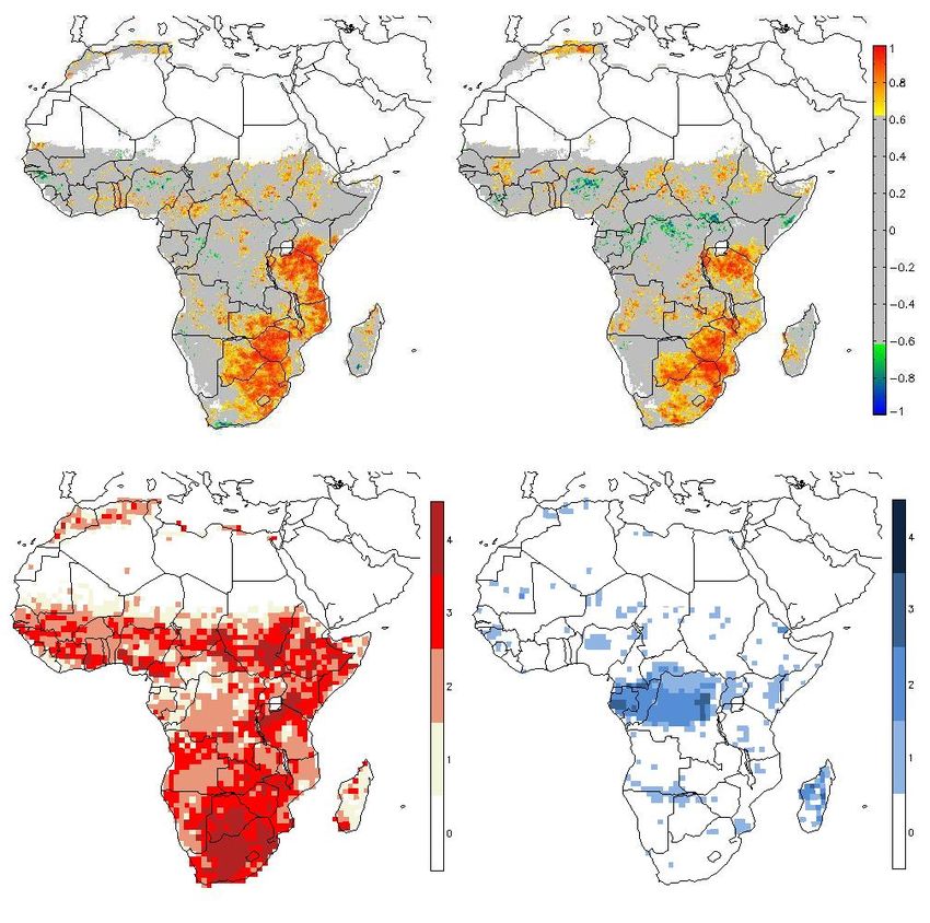
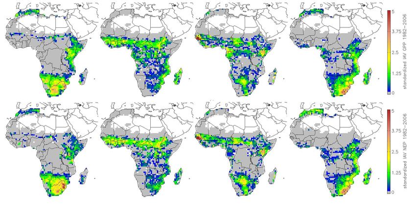
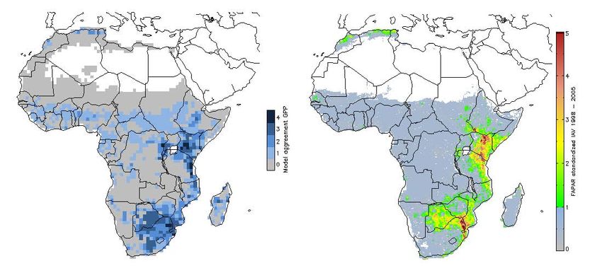
U. Weber et al.: Interannual variability of Africas ecosystem productivity                                                            289

Fig. 2. Comparison of Atmospheric Inversion and Models based on standardized NEP(a) and NBP(b) (1997–2006). Due to the standardiza-
tion method, 0 represents the mean of each individual distribution, but no neutral balance. NEP for models was calculated as the difference
of GPP and TER. NEP from atmospheric inversions was calculated by removing fire emissions using GFED (van der Werf et al., 2006). NBP
refers to the originally inversion results, and NEP minus model specific fire emissions (except JULES, which does not simulate fire).

the Horn of Africa and the South African Grassland are con-             3.2   Regions of large interannual variability
sistent between JULES and LPJ-DGVM, but significantly
lower for ORCHIDEE but in the same range as LPJ-Guess.                  Similar spatial patterns of interannual variability for GPP and
Annual NPP estimates are more consistent between all mod-               NEP are estimated by all models (Fig. 5). Despite some dif-
els. Exceptions are lower LPJ-Guess NPP at the Northern                 ferences of the patterns among the models, we can identify
Savannah Belt, twice as much higher ORCHIDEE NPP than                   areas of large interannual variability of GPP and NEP in east
inter-model average at the Central Tropical Forest, as well             and south Africa predicted by all models (Fig. 6). Both re-
as a high and low plateau situation in the South African                gions are dominated by herbaceous vegetation, including ex-
Grassland region as represented by JULES/LPJ-DGVM and                   tensive agricultural land, and are known to be strongly influ-
ORCHIDEE/LPJ-GUESS.                                                     enced by El Nino conditions (Plisnier et al., 2003; Kogan,
   Despite the discrepancies among models regarding the ab-             2000). The independent remote sensing based FAPAR data
solute flux magnitudes, consistent patterns emerge between              confirms these two variability hotspot regions (Fig. 7). How-
models and with satellite observations regarding seasonal               ever, ORCHIDEE and JULES further simulate considerable
changes of photosynthesis in the different regions (Fig. 4).            variability in the northern savannahs and partly in the tropical
Both, remotely sensed FAPAR and simulated GPP show that                 forest, which is not evident in the satellite observations.
the seasonality of photosynthesis varies in concert with rain-
fall in all regions except for the inner tropical forest, where         3.3   What drives NEP interannual variability – Photosyn-
low intra-annual variation of rainfall creates climatic con-                  thesis or respiration?
ditions without water limitation, reducing the effect of pre-
cipitation on photosynthesis. The heterogeneous vegetation              The previous section indicated that regions of large inter-
of Madagascar together with known extensive anthropogenic               annual NEP variability are associated with also large GPP
transformations (Green and Sussman, 1990) are likely a ma-              variability, suggesting that variations of photosynthesis are
jor reason for the disagreement between the models and be-              driving the variations of the net carbon balance. Table 2 fur-
tween models and remotely sensed FAPAR.                                 ther shows that NEP anomalies in the five defined regions

www.biogeosciences.net/6/285/2009/                                                                   Biogeosciences, 6, 285–295, 2009
290                                                     U. Weber et al.: Interannual variability of Africas ecosystem productivity

                                                                    Table 2. Correlation coefficient (R) between GPP and NEP anoma-
                                                                    lies (left), and TER and NEP anomalies 1 (right) per region and
                                                                    model

                                                                       Northern Savannah Belt            R (GPP/NEP)      R (TER/NEP)
                                                                       LPJ DGVM                          0.71             0.19
                                                                       LPJ GUESS                         0.97             0.82
                                                                       ORCHIDEE                          0.83             0.67
                                                                       JULES                             0.99             0.99
                                                                       Central African tropical forest   R (GPP / NEP)    R (TER / NEP)
                                                                       LPJ DGVM                          0.83             0.57
                                                                       LPJ GUESS                         0.92             0.67
                                                                       ORCHIDEE                          0.79             0.63
                                                                       JULES                             0.94             0.91
                                                                       Horn of Africa                    R (GPP/NEP)      R (TER/NEP)
                                                                       LPJ DGVM                          0.94             0.84
                                                                       LPJ GUESS                         0.99             0.92
                                                                       ORCHIDEE                          0.82             0.60
                                                                       JULES                             0.99             0.99
                                                                       Southern raingreen woodland       R (GPP/NEP)      R (TER/NEP)
                                                                       LPJ DGVM                          0.89             0.64
                                                                       LPJ GUESS                         0.99             0.91
                                                                       ORCHIDEE                          0.47             0.12
                                                                       JULES                             0.96             0.93
                                                                       South African Grassland           R (GPP/NEP)      R (TER/NEP)
                                                                       LPJ DGVM                          0.94             0.78
                                                                       LPJ GUESS                         1.00             0.96
Fig. 3. Annual average GPP, NPP, and NEP per region (g C/m2 /yr).
                                                                       ORCHIDEE                          0.81             0.60
                                                                       JULES                             1.00             0.99

are strongly correlated with GPP anomalies in all models. In
many cases anomalies of ecosystem respiration are also pos-
itively correlated with the NEP anomalies which may appear          Table 3. Eigenvectors and percent variance per Principal Compo-
counterintuitive at first glance. If respiration would drive        nent Modes
the carbon balance we would expect negative correlations;
the positive correlations instead originate from the tight cou-       Eigenvectors   precipitation   temp2m   iswrad   shumid   variance %
pling of GPP and TER in the models, which is also evident             Mode 1         0.41            0.20     −0.26    0.42     55.09
in eddy-covariance based, estimates of GPP and TER (e.g.              Mode 2         0.00            −0.79    −0.61    −0.01    25.19
Reichstein et al., 2007; Baldocchi, 2008). In such case a pos-        Mode 3         −0.51           0.67     −0.87    −0.35    15.57
                                                                      Mode 4         1.67            0.14     −0.15    −1.79    4.14
itive anomaly of TER results in a positive anomaly of NEP
because the GPP increase is even higher, than the (GPP in-
duced) TER stimulation.
   Although the overall pattern of GPP controlled NEP in-
terannual variability is robust and consistent among models         component analysis to reduce the dimensionality of the me-
and regions, we find differences in the strength of this re-        teorological dataset and to extract typical weather gradients
lationship depending on the model and region. JULES and             (see Sect. 2.4). The first two modes of the PCA of the annual
LPJ-GUESS show strongest correlations between GPP and               meteorological data explain 80% of its variability (Table 3)
NEP anomalies (RGPP/NEP >0.92) in all regions, while LPJ-           and are used to infer the primary driving factor of GPP in-
DGVM and ORCHIDEE simulate larger inter-regional vari-              terannual variability in the models. The first mode is most
ability and slightly weaker correlations.                           strongly associated with precipitation and specific humidity
                                                                    and thus represents a gradient of moisture availability. The
                                                                    factor loadings of the second mode show that it represents
4   The response of simulated gross primary production              a gradient of increasing temperature and radiation with de-
    to meteorological conditions                                    creasing values of mode 2.
                                                                        The correlation maps between the first principal compo-
Having identified GPP as a crucial driver of the carbon bal-        nent and GPP clearly show that moisture availability is the
ance and the hotspot regions of largest interannual variability     main limiting factor for photosynthesis (Fig. 8). This find-
in east and South Africa, we now infer which meteorological         ing is in conjunction with Williams et al. (2008), who iden-
conditions drive the variability of GPP. We use a principal         tified water stress as the primary governing factor of IAV

Biogeosciences, 6, 285–295, 2009                                                                 www.biogeosciences.net/6/285/2009/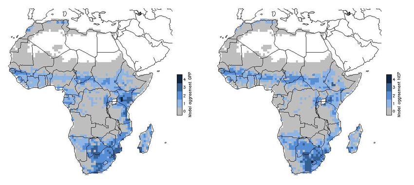
U. Weber et al.: Interannual variability of Africas ecosystem productivity                                                             291

Fig. 4. Standardized mean seasonal cycle GPP from SEAWIFS-FAPAR and participating models.

                                                                        Fig. 7. GPP model agreement of interannual variability defined as
Fig. 5. Standardized interannual variability of modeled GPP (top),      count of models per grid cell where standardized interannual vari-
NEP (bottom); from left: LPJ-DGVM, ORCHIDEE, JULES, LPJ-                ability is greater than one standard deviation 1998–2005 (left), and
GUESS.                                                                  standardized SeaWiFs-FAPAR interannual variability greater one
                                                                        standard deviation 1998–2005 (right)

                                                                        of photosynthesis. Correlation maps between the meteoro-
                                                                        logical PCAs and the mean annual FAPAR from SeaW-
                                                                        iFS (Fig. 9) confirm that primary productivity responds to
                                                                        moisture in south and east Africa, which are the regions of
                                                                        largest interannual variability (see Sect. 3.2). The correla-
                                                                        tions between moisture and FAPAR on interannual scale in
                                                                        the Northern Savannah Belt are not as extensive as indicated
                                                                        by the models. This is possibly an artifact related to the rel-
Fig. 6. Model agreement of interannual variability defined as count
of models per grid cell where standardized interannual variability is   atively short time series (8 years) and coarse meteorological
greater than one standard deviation (GPP (left), NEP (right), 1982–     data. Camberlin et al. (2006) found more widespread strong
2006)                                                                   correlations between integrated NDVI and rainfall for a 20
                                                                        year time series in the northern savannahs. We also find
                                                                        no correlations between moisture and FAPAR in the Horn

www.biogeosciences.net/6/285/2009/                                                                   Biogeosciences, 6, 285–295, 2009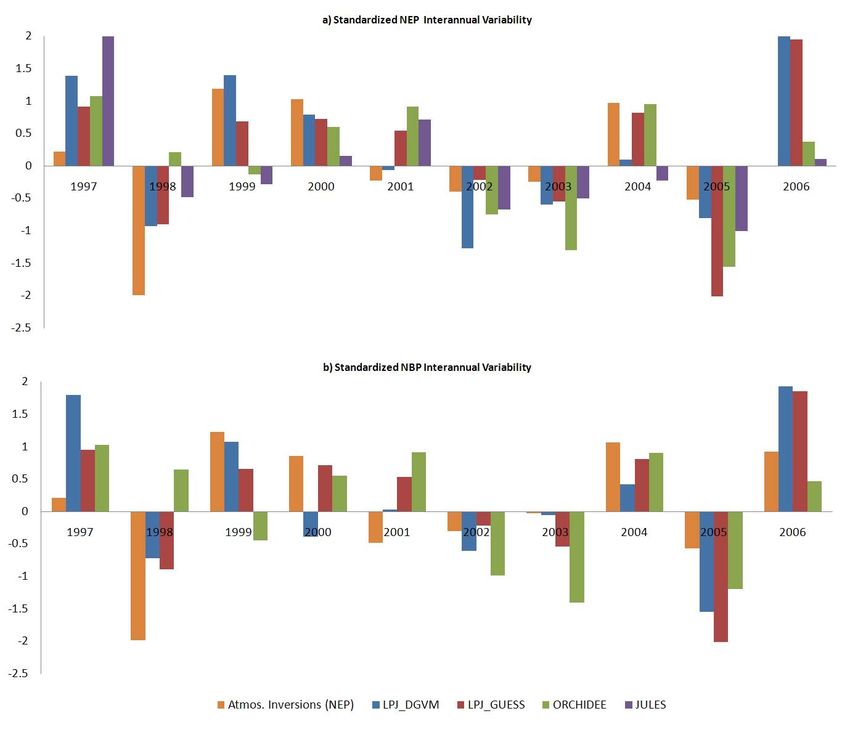
292                                                        U. Weber et al.: Interannual variability of Africas ecosystem productivity

Fig. 8. Correlation between modeled GPP and Meteorology PCA            Fig. 10. Correlation between modeled GPP and Meteorology PCA
1, not significant correlations in grey (confidence interval=0.90)     2, not significant correlations in grey (confidence interval=0.90)

                                                                          The partly different spatial correlation patterns between
                                                                       PCA1 and GPP among the models is likely related to dif-
                                                                       ferent parameterizations for water stress effects such as root
                                                                       profiles, soil depth, and the coupling between photosynthesis
                                                                       and transpiration via canopy conductance which largely de-
                                                                       termines soil water depletion. The simulation of water stress
                                                                       effects on photosynthesis has been previously identified as a
                                                                       major source for differences among models regarding inter-
                                                                       annual variability of GPP in Europe (Jung et al., 2007; Vetter
                                                                       et al., 2008).
                                                                          The general water limitation of African vegetation’s pri-
                                                                       mary production is consistent with Churkina and Run-
                                                                       ning (1998) based on Biome-BGC simulations and Jolly
                                                                       et al. (2005) based on the analysis of remote sensing data
                                                                       from MODIS. Using a production efficiency model Nemani
                                                                       et al. (2003) find that tropical Africa is primarily radiation
                                                                       limited, while both Churkina and Running (1998) as well
                                                                       as Jolly et al. (2005) masked the inner tropical regions and
                                                                       concluded that no climatic constrain limits productivity here.
                                                                       Interestingly, LPJ-DGVM and JULES also suggest that not
Fig. 9. Top: Correlation between FAPAR and Meteorology PCA 1
                                                                       rainfall but radiation limits GPP in some regions, especially
(left) and PCA 2 (right), not significant correlations in grey (con-
                                                                       in the inner tropics. This is represented by the negative
fidence interval=0.90), bottom: Model Agreement of significant
(confidence interval=0.90) positive correlations between PCA1 and      correlations between PCA 2 and GPP in the tropical for-
GPP (left), and of significant negative correlations between PCA2      est where simulated GPP increases with increasing radiation
and GPP (right).                                                       and temperature (Fig. 10). Given that temperature limitation
                                                                       does likely not play a role here, we can interpret the neg-
                                                                       ative correlations between PCA2 and GPP as an indication
of Africa region while the models suggest such relationship.
                                                                       for light limitation. The latter also makes sense since fre-
For this region Camberlin et al. (2006) confirm no correla-
                                                                       quent cloud cover is present in the tropics, which controls
tion between precipitation and vegetation productivity for the
                                                                       incoming radiation with otherwise favorable climatic condi-
northern corner of the African Horn but indicate strong cor-
                                                                       tions for productivity. Light limitation for parts of the Ama-
relations with rainfall in the southern part of the region.
                                                                       zon tropical forests has been inferred from studying wet to

Biogeosciences, 6, 285–295, 2009                                                                www.biogeosciences.net/6/285/2009/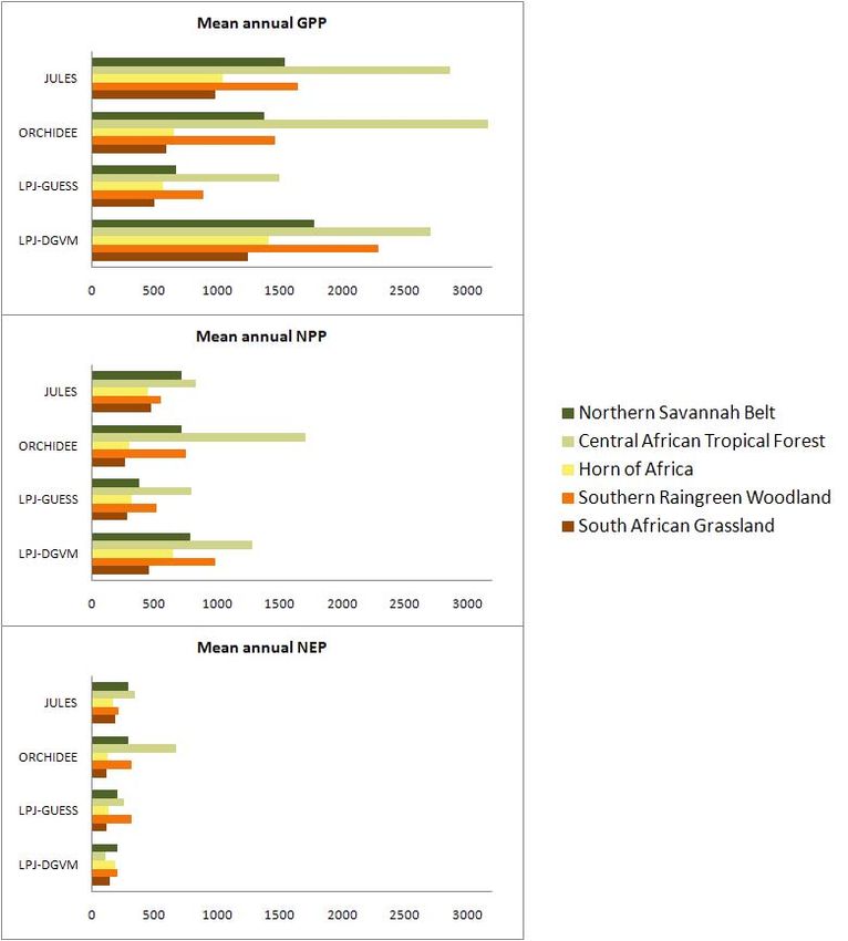
U. Weber et al.: Interannual variability of Africas ecosystem productivity                                                        293

dry season transitions using in-situ measurements of CO2            (Merbold et al., 2009). Given the significance of moisture
gas exchange (Saleska et al., 2003), manipulative experi-           control on the carbon fluxes in most parts of Africa, particu-
ments (Graham et al., 2002), and remote sensing based stud-         lar attention should be dedicated to the models’ ability to ac-
ies (Huete et al., 2006; Xiao et al., 2006; Nemani et al.,          curately simulate soil hydrological conditions, and the sensi-
2003). Light limitation for parts of the Amazon result from         tivity of photosynthesis and soil respiration to soil moisture.
access to groundwater during dry seasons when the vegeta-
tion capitalizes from the increases incoming radiation. From        Acknowledgements. The work was supported by the European
the correlation maps between the remote sensing based FA-           Commission via the FP6 project CarboAfrica (EU, Contract No.:
PAR and PCA2 we also find patches in the inner tropics of           037132). We thank Neil Hanan and Christopher Williams for their
Africa where productivity increases with increasing radiation       support on the experimental setup and implementation.
but to a much smaller extent than suggested by some of the
models. Thus, the role of light availability in the African         Edited by: F. Joos
tropics remains controversial. There are several possible rea-
sons why we find only small areas with significant corre-
                                                                                           This Open Access Publication is
lation between radiation and productivity from the remote                                  financed by the Max Planck Society.
sensing data: (1) the short time series (8 years) in combina-
tion with small variances make it difficult to achieve large
correlations, (2) the uncertainty of the meteorological data
that originate from global reanalysis, (3) possible errors in
the satellite FAPAR retrievals due to subpixel cloud contam-        References
ination, (4) a strong role of non-climatic limitations of pro-
ductivity such as nutrients. If nutrients are not most limiting,    Anyamba, A., Tucker, C. J., and Mahoney, R.: From El Niño to
ecosystems are more sensitive to climatic variations. Possi-          La Niña: Vegetation Response Patterns over East and Southern
bly, light limitation in the African tropics occurs where less        Africa during the 1997–2000 Period, J. Clim., 15(21), 3096–
phosphorous depleted soils are present since phosphorous is           3103, 2002
believed to be generally the main limiting factor for produc-       Anyamba, A., Justice, C. O., Tucker, C. J., and Mahoney, R.: Sea-
                                                                      sonal to interannual variability of vegetation and fires at SA-
tivity in the tropics (Vitousek, 1984). The overriding effect
                                                                      FARI 2000 sites inferred from advanced very high resolution
of nutrient availability may explain why we find only small           radiometer time series data, J. Geophys. Res., 108(D13), 8507,
areas with light limitation from the analysis using the satel-        doi:10.1029/2002JD002464, 2003.
lite data, in contrast to the extensive areas of light limitation   Baldocchi, D.: ’Breathing’ of the terrestrial biosphere: lessons
indicated by LPJ-DGVM, JULES, and Nemani et al. (2003)                learned from a global network of carbon dioxide flux measure-
because none of the latter considers explicitly nutrient cycles.      ment systems, Australian J. Botany, 56, 1–26, 2008.
                                                                    Camberlin, P., Martiny, N., Philippon, N., and Richar, Y.: Deter-
                                                                      minants of the interannual relationships between remote sensed
5   Conclusions                                                       photosynthetic activity and rainfall in tropical Africa. Remote
                                                                      Sens. Environ., 106(2), 199–216, 2006.
Using four terrestrial ecosystem models in combination with         Cao, M. K., Zhang, Q. F., and Shugart, H. H.: Dynamic responses
remote sensing based information of vegetation productivity           of African ecosystem carbon cycling to climate change, Clim.
                                                                      Res., 17, 183–193, 2001.
we were able to identify that (1) the largest interannual vari-
                                                                    Churkina, G. and Running, S.: Contrasting climatic controls on the
ability of gross primary production and net ecosystem pro-            estimated productivity of global terrestrial biomes, Ecosystems,
ductivity are concentrated in east and south Africa, (2) inter-       1, 206–215, 1998.
annual variations of gross primary production is driving net        Ciais, P., Reichstein, M., Viovy, N., Granier, A., Oge’e, J., Al-
ecosystem production in the models, and (3) the availability          lard, V., Aubinet, M., Buchmann, N., Bernhofer, Chr., Carrara,
of moisture is the primary determinant of interannual varia-          A., Chevallier, F., De Noblet, N., Friend, A. D., Friedlingstein,
tions of gross primary production and consequently the net            P., Gruenwald, T., Heinesch, B., Keronen, P., Knohl, A., Krin-
carbon balance.                                                       ner, G., Loustau, D., Manca, G., Matteucci, G., Miglietta, F.,
   Nevertheless, our current simulations reveal substantial           Ourcival, J. M., Papale, D., Pilegaard, K., Rambal, S., Seufert,
discrepancies among models regarding the actual flux mag-             G., Soussana, J. F., Sanz, M. J., Schulze, E. D., Vesala, T.,
                                                                      and Valentini, R.: Europe-wide reduction in primary produc-
nitudes. Future simulations should be performed with im-
                                                                      tivity caused by the heat and drought in 2003, Nature, 437,
proved forcings by prescribing the actual distribution of veg-        doi:10.1038/nature03972, 2005.
etation types provided by a remote sensing based land cover         Collatz, G. J., Ball, J. T., Grivet, C., and Berry, J. A.: Physio-
map and improved meteorological reanalysis. In addition it            logical and environmental-regulation of stomatal conductance,
should be investigated to what extent the models are able to          photosynthesis and transpiration a model that includes a lami-
reproduce the ecological patterns found in the synthesis of in-       nar boundary-layer, Agric. Forest Meteorol., 54(2–4), 107–136.
situ measurements of carbon and water fluxes across Africa            1991.

www.biogeosciences.net/6/285/2009/                                                              Biogeosciences, 6, 285–295, 2009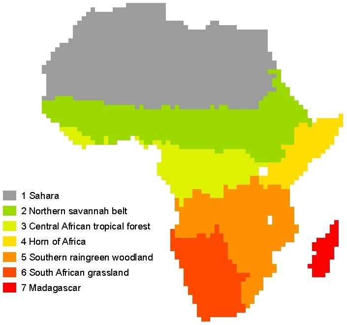
294                                                          U. Weber et al.: Interannual variability of Africas ecosystem productivity

Collatz, G. J., Ribas-Carbo, M., and Berry, J. A.: Coupled               IPCC 2007: Climate Change 2007: The Physical Science Basis.
   photosynthesis-stomatal conductance model for leaves of C4               Contribution of Working Group I to the Fourth Assessment Re-
   plants, Aust. J. Plant Physiol., 19(5), 519–538, 1992.                   port of the Intergovernmental Panel on Climate Changem, edited
Cox, P. M.: Description of the TRIFFID Dynamic Global Vegeta-               by: Solomon, S., Qin, D., Manning, M., Chen, Z., Marquis, M.,
   tion Model. Technical Note 24. Hadley Centre, Met Office, UK,            Averyt, K. B., Tignor, M., and Miller, H. L., Cambridge Univer-
   16, 2001.                                                                sity Press, Cambridge, UK and New York, NY, USA.
Cramer, W., Kicklighter, D. W., Bondeau, A., Moore, B., Churkina,        Jung, M., Vetter, M., Herold, M., Churkina, G., Reichstein, M., Za-
   G., Nemry, B., Ruimy, A., and Schloss, A. L.: Comparing global           ehle, S., Cias, P., Viovy, N., Bondeau, A., Chen, Y., Trusilova,
   models of terrestrial net primary productivity (NPP): overview           K., Feser, F., and Heimann, M.: Uncertainties of modelling GPP
   and key results, Glob. Change Biol., 5, 1–15. 1999.                      over Europe: A systematic study on the effects of using differ-
Cramer, W., Bondeau, A., Woodward, F. I., Prentice, I. C., Betts,           ent drivers and terrestrial biosphere models, Global Biogeochem.
   R. A., Brovkin, V., Cox, P. M., Fisher, V., Foley, J., Friend,           Cy., 21, GB4021, doi:10.1029/2006GB002915, 2007.
   A. D., Kucharik, C., Lomas, M. R., Ramankutty, N., Sitch, S.,         Jung, M., Verstraete, M., Gobron, N., Reichstein, M., Papale, D.,
   Smith, B., White, A., and Young-Molling, C.: Global response             Bondeau, A., Robustelli, M., and Pinty, B.: Diagnostic assess-
   of terrestrial ecosystem structure and function to CO2 and cli-          ment of European gross primary production, Global Change Bi-
   mate change: results from six dynamic global vegetation models,          ology, 14, 1–16, doi:10.1111/j.1365-2486.2008.01647.x, 2008.
   Glob. Change Biol., 7(4), 357–373. 2001.                              Jolly, W., Nemani, R., and Running, S. W.: A generalized, bio-
Essery, R. L. H., Best, M. J., and Cox, P. M.: MOSES 2.2 Technical          climatic index to predict foliar phenology in response to cli-
   Documentation. Technical Note 30. Hadley Centre, Met Office,             mate, Global Change Biol., 11, 619–632, doi:10.1111/j.1365-
   UK, 30, 2001.                                                            2486.2005.00930.x, 2005.
Farquhar, G. D., von Caemmerer, S., and Berry, J. A.: A biogeo-          Kalnay, E., Kanamitsu, M., Kistler, R., Collins, W., Deaven, D.,
   chemical model of photosynthesis in leaves of C3 species. Planta,        Gandin, L., Iredell, M., Saha, S., White, G., Woollen, J.Zhu,
   149, 78–90, 1980.                                                        y., Chelliah, M., Ebisuzaki, W., Higgins, W., Janowiak, J., Mo,
Fekete, B. M., Vörösmaty, C. J., Roads, J.O., and Willmott, C. J.:        K.C., Ropelewski, C., Wang, J., Leetmaa, A., and Reynolds, R.:
   Uncertainties in Precipitation and Their Impacts o Runoff Esti-          The NCEP/NCAR 40-year reanalysis project, B. Amer. Meteor.
   mates, J. Climate, 17, 294–304. 2003.                                    Soc., 77, 437–470, 1996.
Friedlingstein, P., Cox, P., Betts, R., Bopp, L., Von Bloh, W.,          Kanamitsu, M., Ebisuzaki, W., Woollen, J., Yang, S.-K., Hnilo,
   Brovkin, V., Cadule, P., Doney, S., Eby, M., Fung, I., Bala, G.,         J. J., Fiorino, M., and Potter, G. L.: NCEP-DEO AMIP-
   John, J., Jones, C., Joos, F., Kato, T., Kawamiya, M., Knorr,            II Reanalysis (R-2), B. Atmos. Meterol. Soc., 1631–1643,
   W., Lindsay, K., Matthews, H. D., Raddatz, T., Rayner, P., Re-           doi:10.1175/BAMS-83-11-1631, November 2002.
   ick, C., Roeckner, E., Schnitzler, K. G., Schnur, R., Strassmann,     Kistler,R., Kalnay, E., Collins,W., Saha,S., White,G., Woollen,J.,
   K., Weaver, A. J., Yoshikawa, C., and Zeng, N.: Climate-carbon           Chelliah, M., Ebisuzaki, W., Kanamitsu, M., Kousky, V., van
   cycle feedback analysis: Results from the (CMIP)-M-4 model               den Dool, H., Jenne, R., and Fiorino, M.: The NCEP–NCAR 50-
   intercomparison, J. Clim., 19, 3337–3353, 2006.                          Year Reanalysis: Monthly Means CD-ROM and Documentation.
Foley, J. A., Prentice, I. C., Ramankutty, N., Levis, S., Pollard, D.,      B. Am. Meteorol. Soc., 82, 247–267. 2001.
   Sitch, S., and Haxeltine, A.: An integrated biosphere model of        Kogan, F. N.: Satellite – Observed Sensitivity of World Land
   land surface processes, terrestrial carbon balance and vegetation        Ecosystems to El Niño/La Niña, Remote Sens. Environ., 74,
   dynamics, Global Biogeochem. Cy., 10( 4), 603–628, 1996.                 445–462, 2000.
Gobron, N., Pinty, B., Verstraete, M. M., and Widlowski, J.-L.:          Krinner, G., Viovy, N., de Noblet-Ducoudre, N., Ogee, J., Polcher,
   Advanced vegetation indices optimized for up-coming sensors:             J., Friedlingstein, P., Ciais, P., Stitch, S., and Prentice, C.: A dy-
   Design, performance, and applications, Geosci. Remote Sens.,             namic global vegetation model for studies of the coupled atmo-
   38(6), 2489–2505, 2000.                                                  sphere biosphere system, Global Biogeochem. Cy., 19, GB1015,
Gobron, N., Pinty, B., Mélin, F., Taberner, M., Verstraete, M. M.,         doi:10.1029/2003GB002199. 2005.
   Belward, A., Lavergne, T., and Widlowski, J.-L.: The state of         Kummerow, C., Barnes, W., Kozu, T., Shiue, J., and Simpson, J.:
   vegetation in Europe following the 2003 drought, Int. J. Remote          The Tropical Rainfall Measuring Mission (TRMM) sensor pack-
   Sens. Lett., 26, 2013–2020, 2005.                                        age, J. Atmos. Ocean. Tech., 15, 809–817, 1998.
Graham, F. A., Mulkey, S. S., Kitajima, K., Phillips, N. G., and         Le Page, Y., Pereira, J. M. C., Trigo, R., Da Camara, C., Oom,
   Wright, S. S.: Cloud cover limits net CO2 uptake and growth              D., and Mota, B.: Global fire activity patters (1996–2006)
   of a rainforest tree during tropical rainy seasons, PNAS, 100(2),        and climatic influence: an analysis using the World Fire Atlas,
   572–576, 2003.                                                           Atmos. Chem. Phys., 8, 1911–1924, 2008, http://www.atmos-
Green, G. M. and Sussman, R. W.: Deforestation history of the               chem-phys.net/8/1911/2008/.
   eastern rain forests of Madagascar from satellite images, Science,    Linacre, E. T.: Net Radiation to Various Surfaces, J. Appl. Ecol.,
   248, 212–215, 1990.                                                      6(1), 61–75, 1969.
Huete, A. R., Didan, K., Shimabukuro, Y. E., Ratana, P., Saleska,        Lloyd, J. and Taylor, J. A.: On the temperature dependence of soil
   S. R., Hutyra, L. R., Yang, W., Nemani, R. R., and Myneni, R.:           respiration, Funct. Ecol. 8, 315–323, 1994.
   Amazon rainforests green-up with sunlight in dry season, Geo-         McGuire, A. D., Sitch, S., Clein, J. S., Dargaville, R., Esser, G., Fo-
   phys. Res. Lett., 33, L06405, doi:10.1029/2005GL025583, 2006             ley, J., Heimann, M., Joos, F., Kaplan, J., Kicklighter, D. W.,
Hughes, J. K., Valdes, P. J., and Betts, R.: Dynamics of a global-          Meier, R. A., Melillo, J. M., Moore, B., Prentice, I. C., Ra-
   scale vegetation model, Ecol. Model., 198(3–4), 452–462, 2006.           mankutty, N., Reichenau, T., Schloss, A., Tian, H., Williams,

Biogeosciences, 6, 285–295, 2009                                                                    www.biogeosciences.net/6/285/2009/
U. Weber et al.: Interannual variability of Africas ecosystem productivity                                                                  295

   L. J., and Wittenberg, U.: Carbon balance of the terrestrial           Sheffield, J., Goteti, G., and Wood, E. F.: Development of a 50-year
   biosphere in the twentieth century: Analyses of CO2 , climate             High Resolution Global Dataset of Meteorological Forcings for
   and land use effects with four process-based ecosystem models,            Land Surface Modeling, J. Clim., 19, 3088–3110, 2006.
   Global Biogeochem. Cy., 15, 183–206, 2001                              Sitch, S., Smith, B., Prentice, I. C., Arneth, A., Bondeau, A.,
Mitchell, T. D. and Jones, P. D.: An improved method of con-                 Cramer, W., Kaplan, J. O., Levis, S., Lucht, W., Sykes, M. T.,
   structing a database of monthly climate observations and as-              Thonicke, K., and Venevsky, S.: Evaluation of ecosystem dy-
   sociated high-resolution grids, Int. J. Climatol., 25, 693–712,           namics, plant geography and terrestrial carbon cycling in the LPJ
   doi:10.1002/joc.1181, 2005.                                               dynamic global vegetation model, Glob. Change Biol., 9, 161–
Morales, P., Sykes, M. T., Prentice, I. C., Smith, P., Smith, B., Bug-       185, 2003.
   mann, H., Zierl, B., Friedlingstein, P., Viovy, N., Sabaté, S.,       Smith, T. M., Shugart, H. H. and Woodward, F. I. (Eds.): Plant
   Sánchez, A., Pla, E., Gracia, C. A., Sitch, S.,Arneth, A., and           Functional Types, Cambridge University Press, Cambridge,
   Ogee, J.: Comparing and evaluating process-based ecosystem                1997.
   model predictions of carbon and water fluxes in major European         Smith, B., Prentice, I. C., and Sykes, M. T.: Representation of
   forest biomes, Global Change Biol., 11, 1–23, 2005.                       vegetation dynamics in the modelling of terrestrial ecosystems:
Myneni, R. B., Los, S. O., and Tucker, C. J.: Satellite based identi-        comparing two contrasting approaches within European climate
   fication of linked vegetation index and sea surface anomaly areas         space, Global Ecol. Biogeogr., 10, 621–637, 2001.
   from 1982–1990 for Africa, Australia and South America, Geo-           Shugart, H. H.: A Theory of Forest Dynamics: The Ecological Im-
   phys. Res. Lett., 23(7), 729–732, 1996.                                   plications of Forest Succession Models, Springer-Verlag, New
Nemani, R. R., Keeling, C. D., Hashimoto, H., Jolly, W. M.,                  York, USA, 1984.
   Piper, S. C., Tucker, C. T., Myneni, R. B., and Running, S.            Tempel, P., Batjes, N. H., Collaty, G. J., and van Engelen, V. W. P.:
   W.: Climate-Driven Increases in Global Terrestrial Net Pri-               IGBP-DIS soil data set for pedotransfer function development,
   mary Production from 1982 to 1999, Science, 300, 5625,                    Working paper and Reprint 96/05, International Soil Reference
   doi:10.1126/science.1082750, 2003.                                        and Information Centre (ISRIC), Wageningen, 1996.
Ngo-Duc, T., Polcher, J., and Laval, K.: A 53-year data                   TRMM 3B43- Tropical Rainfall Measuring Mission Science Data
   set for land surface models, J. Geophy.Res., 110, D06116,                 and Information System (TSDIS) Interface Control Specifica-
   doi:101029/2004JD005434, 2005.                                            tion: ftp://disc2.nascom.nasa.Gov/data/TRMM/Gridded/3B43
Plisnier, P. D., Serneels, S., and Lambin, E. F.: Impact of ENSO             V6/, last access: 31 May 2007.
   on East African ecosystems: a multivariate analysis based on cli-      Thonicke, K., Venevsky, S., Sitch, S., and Cramer, W.: The role
   mate and remote sensing data, Global Ecol. Biogeogr., 9, 481–             of fire disturbance for global vegetation dynamics: coupling fire
   497, 2000.                                                                into a Dynamic Global Vegetation Model, Global Ecol. Bio-
Potter, C. S., Klooster, S., and Brooks, V.: Interannual variability in      geogr., 10, 661–677, 2001.
   terrestrial net primary production: Exploration of trends and con-     Van der Werf, G. R., Randerson, J. T., Giglio, L., Collatz, G. J.,
   trols on regional to global scales, Ecosystems, 2, 36–48, 1999.           and Kasibhatla, P. S.: Interannual variability in global biomass
Potter, C., Klooster, S., Myneni, R., Genovese, V., Tan, P.-N.,              burning emission from 1997 to 2004, Atmos. Chem. Phys., 6,
   and Kumar, V.: Continental-scale comparisons of terrestrial car-          3423–3441. 2006.
   bon sinks estimated from satellite data and ecosystem modeling         Vetter, M., Churkina, G., Jung, M., Reichstein, M., Zaehle, S.,
   1982–1998, Glob. Planet. Change, 39, 201–213, 2003.                       Bondeau, A., Chen, Y. H., Ciais, P., Feser, F., Freibauer, A.,
Randerson, J. T., van der Werf, G. R., Giglio, L., Collatz, G. J.,           Geyer, R., Jones, C., Papale, D., Tenhunen, J., Tomelleri, E.,
   and Kasibhatla, P. S.: Global Fire Emissions Database, Version            Trusilova, K., Viovy, N., and Heimann, M.: Analyzing the
   2 (GFEDv2.1), Data set, available online: http://daac.ornl.gov/           causes and spatial pattern of the European 2003 carbon flux
   from Oak Ridge National Laboratory Distributed Active Archive             anomaly using seven models, Biogeosciences, 5, 561–583, 2008,
   Center, Oak Ridge, Tennessee, USA, 2007.                                  http://www.biogeosciences.net/5/561/2008/.
Reichstein, M., Papale, D., Valentini, R., Aubinet, M., Bernhofer,        Vitousek, M.: Litterfall, Nutrient Cycling, and Nutrient Limitation
   C:, Knohl, A., Laurila, T., Lindroth, A., Moors, E., Pilegaard,           in Tropical Forests, Ecology, 65, 285–298, 1984.
   K., and Seufert, G.: Determinants of terrestrial ecosystem carbon      Williams, C. W., Hanan, N. P., Neff, J. C., Scoles, R. J., Berry, J. A.,
   balance inferred from European eddy covariance flux sites, Geo-           Denning, A. S., and Baker, D. F.: Africa and the global carbon
   phys. Res. Lett., 34, L01402262, doi:10.1029/2006GL027880,                cycle, Carbon Balance and Management, 2:3, doi:10.1186/1750-
   2007.                                                                     0680-2-3, 2007.
Rödenbeck, C.: Estimating CO2 sources and sinks from atmo-               Williams, C. A., Hanan, N. P., Baker, I., Collatz, G. J., Berry, J.,
   spheric mixing ratio measurements using a global inversion of             and Denning, A. S.: Interannual variability of photosynthesis
   atmospheric transport. Technical Report 6, Max Planck Institute           across Africa and its attribution, J. Geophys. Res., 113, G04015,
   for Biogeochemistry, Jena, 61, 2005.                                      doi:10.1029/2008JG000718, 2008.
Saleska, S. R., Miller, S. D., Matross, D. M., Goulden, M. L.,            Xiao, X., Hagen, S., Zhang, Q., Keller, M., and Moore III, B.:
   Wofsy, S. C., Da Rocha, H. R., De Camargo, P. B., Crill, P.,              Detecting leaf phenology of seasonally moist tropical forests
   Daube, B. C., De Freitas, H. C., Hutyra, L., Keller, M., Kirch-           in South America with multi-temporal MODIS images, Remote
   hoff, V., Menton, M., Munger, J. W., Hammond Pyle, E., Rice, A.           Sens. Environ., 103, 465–473, 2006.
   H., and Silva, H.: Carbon in Amazon Forest: Unexpected Sea-            Trends in Atmospheric Carbon Dioxide – Mauna Loa: www.esrl.
   sonal Fluxes and Disturbance – Induced Losses. Science, 302,              noaa.gov/gmd/ccgg/trends/, access: 12 July 2007.
   1554–1557, 2003.

www.biogeosciences.net/6/285/2009/                                                                       Biogeosciences, 6, 285–295, 2009
You can also read