Long Island Sound temperature variability and its associations with the ridge-trough dipole and tropical modes of sea surface temperature ...
←
→
Page content transcription
If your browser does not render page correctly, please read the page content below
Ocean Sci., 15, 161–178, 2019
https://doi.org/10.5194/os-15-161-2019
© Author(s) 2019. This work is distributed under
the Creative Commons Attribution 4.0 License.

Long Island Sound temperature variability and its associations with
the ridge–trough dipole and tropical modes of sea surface
temperature variability
Justin A. Schulte1 and Sukyoung Lee2
1 Science   Systems and Applications, Inc., Lanham, Maryland, 20706, USA
2 Department    of Meteorology, The Pennsylvania State University, University Park, 16802, USA

Correspondence: Justin A. Schulte (justin.a.schulte@nasa.gov)

Received: 2 March 2018 – Discussion started: 19 March 2018
Revised: 4 October 2018 – Accepted: 11 October 2018 – Published: 21 February 2019

Abstract. Possible mechanisms behind the longevity of in-         1   Introduction
tense Long Island Sound (LIS) water temperature events are
examined using an event-based approach. By decomposing            Fluctuations in sea surface temperature (SST) across coastal
an LIS surface water temperature time series into negative        portions of the United States (US) are driven by changes
and positive events, it is revealed that the most intense LIS     in oceanic and atmospheric circulation patterns. Changes in
water temperature event in the 1979–2013 period occurred          water temperature along the US west coast are related to
around 2012, coinciding with the 2012 ocean heat wave             the Pacific Decadal Oscillation (PDO) and the North Pacific
across the Mid-Atlantic Bight. The LIS events are related to      Gyre Oscillation, as is well documented (Mantua et al., 1997;
a ridge–trough dipole pattern whose strength and evolution        Mantua and Hare, 2002; Di Lorenzo, 2008). For the US east
can be determined using a dipole index. The dipole index was      coast, water temperature fluctuations are related to changes
shown to be strongly correlated with LIS water temperature        in the Gulf Stream position and variations in the Atlantic
anomalies, explaining close to 64 % of cool-season LIS water      Multidecadal Oscillation, PDO, and East Pacific–North Pa-
temperature variability. Consistently, a major dipole pattern     cific (EP–NP) pattern (Pershing et al., 2015; Schulte et
event coincided with the intense 2012 LIS warm event. A           al., 2018). Superimposed on the water temperature changes
composite analysis revealed that long-lived intense LIS wa-       driven by natural modes of variability is background warm-
ter temperature events are associated with tropical sea surface   ing associated with anthropogenic climate change (Pershing
temperature (SST) patterns. The onset and mature phases of        et al., 2015).
LIS cold events were shown to coincide with central Pa-              Although the mechanisms behind SST variability along
cific El Niño events, whereas the termination of LIS cold         the US west coast are well documented, comparatively fewer
events was shown to possibly coincide with canonical El           studies have focused on understanding SST variability across
Niño events or El Niño events that are a mixture of eastern       the Mid-Atlantic Bight in the context of large-scale climate
and central Pacific El Niño flavors. The mature phase of LIS      modes. Two recent studies put water temperature variabil-
warm events was shown to be associated with negative SST          ity across the Gulf of Maine and the Long Island Sound
anomalies across the central equatorial Pacific, though the re-   (LIS) in a climate-mode context. The first study by Persh-
sults were not found to be robust. The dipole pattern was also    ing et al. (2015) showed that the combination of Gulf Stream
shown to be related to tropical SST patterns, and fluctuations    and PDO influences led to the rapid warming of the Gulf of
in central Pacific SST anomalies were shown to evolve co-         Maine that resulted in the collapse of the cod fishery.
herently with the dipole pattern and the strongly related East       More recently, a second study by Schulte et al. (2018)
Pacific–North Pacific pattern on decadal timescales. The re-      found the EP–NP pattern to be a dominant pattern govern-
sults from this study have important implications for seasonal    ing LIS water temperature variability. The EP–NP pattern
and decadal prediction of the LIS thermal system.                 was shown to be strongly correlated with LIS water tem-

Published by Copernicus Publications on behalf of the European Geosciences Union.
162                                                    J. A. Schulte and S. Lee: Long Island Sound temperature variability

perature unlike the well-known North Atlantic Oscillation         general movement of weather systems from west to east may
(NAO; Hurrell, 1995), Pacific North American (PNA; Wal-           reflect the weak NAO influences because the NAO’s centers
lace and Gutzler, 1981; Svoma, 2011), Arctic Oscillation          of action are located downstream of the LIS.
(AO; Thompson and Wallace, 1998), and West Pacific (WP;              Recognizing that well-known climate indices are weakly
Barston and Livezey, 1987; Linkin and Nigam, 2008) pat-           related to the salinity variability of northeast US estuar-
terns. In fact, Schulte and Lee (2017) found that the EP–         ies, Schulte et al. (2017a) adopted a continuum approach
NP pattern is more strongly related to temperature variability    (Franzke and Feldstein, 2005; Johnson and Feldstein, 2010;
across the northeast US than the AO, which is often asso-         Johnson et al., 2008) to teleconnection pattern extraction
ciated with colder-than-normal conditions across the region       and identified an eastern North American (ENA) sea level
(Wettstein and Mearns, 2002). Those results suggest that the      dipole pattern that is more strongly correlated with stream-
EP–NP pattern is an important component to seasonal pre-          flow than the PNA and NAO indices. In a subsequent study,
diction of air and water temperature across the LIS region.       Schulte et al. (2017b) found the ENA pattern to be strongly
Another important aspect of the EP–NP pattern is its strong       related to northeast US precipitation and LIS salinity. Those
decadal variability, which could enable decadal prediction        results suggest that a continuum approach is better suited
of LIS water temperature. Schulte et al. (2018) termed the        for understanding climate variability and associated LIS wa-
decadal component of the EP–NP pattern the quasi-decadal          ter temperature impacts than an EOF-based analysis. Al-
mode and showed that it fluctuates coherently with LIS water      though Schulte et al. (2018) did show that the EOF-based
temperature anomalies. The physical mechanism contribut-          EP–NP pattern is strongly correlated with LIS water tem-
ing to the EP–NP decadal variability was not identified, un-      perature, the EP–NP pattern for December cannot be unam-
derscoring the need for an additional study to identify a pos-    biguously extracted using the rotated principal component
sible source of the EP–NP decadal variability. Understand-        analysis (RPCA) conducted by the Climate Prediction Center
ing the mechanisms behind the EP–NP decadal variability           (CPC). Furthermore, EOF analysis assumes atmospheric pat-
has implications for seasonal and decadal prediction of LIS       terns are orthogonal even though orthogonality does not hold
water temperature.                                                for the real atmosphere. This orthogonality assumption can
   Improving the current understanding of the climatic mech-      lead to the generation of unphysical modes (Tremblay, 2001).
anisms governing LIS water temperature variability also has       In contrast, clustering methods such as self-organizing maps
important implications for managing fisheries. For example,       (SOMs) that view the atmosphere as a continuum more accu-
Howell and Auster (2012), using finfish abundance indices,        rately produce patterns that are actually observed than EOF
found shifts in spring community structures that are related to   analysis (Liu et al., 2006; Johnson et al., 2008; Yuan et al.,
water temperature. The LIS American lobster, which is sensi-      2015).Therefore, an additional study is needed to construct
tive to water temperature, dramatically declined around 1997      an atmospheric circulation index that is strongly related to
(Pearce and Balcom, 2005), but managing the lobster har-          LIS water temperature variability, physically based, and un-
vests has failed to recover the lobster fishery. For the nearby   ambiguously defined for all months.
Rhode Island Sound, biological communities are related to            In this paper, we use an event-based approach to iden-
spring–summer water temperature (Collie et al., 2008), sug-       tify LIS water temperature relationships with atmospheric
gesting that predicting spring–summer water temperature           and oceanic patterns. More specifically, the main objectives
could aid the setting of fish harvest quotas. These studies       of the study are the following: (1) identify the atmospheric
underscore the need to better understand water temperature        circulation patterns associated with LIS water temperature
variability across the LIS region so that changes in biologi-     events; (2) create a simple atmospheric index that is strongly
cal communities can be better monitored and used to better        correlated with LIS water temperature; and (3) use the sim-
manage fish harvests.                                             ple atmospheric index to better understand LIS water temper-
   Another reason that the LIS is important to study is that it   ature variability. Because tropical Pacific SST patterns are
is in a region where air temperature and precipitation are not    often used in seasonal forecasting over North America, we
strongly influenced by well-known climate modes such as the       address the question as to whether there is an SST pattern
NAO, AO, PNA, and WP that are extracted from the widely           precursor to LIS temperature events.
used classical empirical orthogonal function (EOF) analysis
method (Barston and Livezey, 1987). Schulte et al. (2016)
found weak relationships between well-known climate in-           2   Data
dices and the variability of precipitation and temperature
across the northeast US. As shown by Schulte et al. (2018),       In this paper, SST fields from 1870 to 2013 are based on
LIS water temperature variability is strongly related to nei-     the Hadley Centre Global Sea Ice and Sea Surface Tem-
ther changes in the Gulf Stream position nor fluctuations         perature (HadISST1) data set (Rayner et al., 2016). At-
in the NAO despite being located adjacent to the Atlantic         mospheric fields were analyzed using 500 hPa geopotential
Ocean. The weak Gulf Stream influence is likely the result        height and sea level pressure (SLP) fields based on the Na-
of the LIS being a semi-enclosed water basin, whereas the         tional Oceanic Atmospheric Administration’s 20th century

Ocean Sci., 15, 161–178, 2019                                                                www.ocean-sci.net/15/161/2019/
J. A. Schulte and S. Lee: Long Island Sound temperature variability                                                                     163

reanalysis (Compo et al., 2011) and the National Center for         (Kao and Yu, 2009; Lee and McPhaden, 2010) Thus, using
Atmospheric Prediction (NCEP; Kalnay et al., 1996) reanal-          these two indices, we accounted for two different flavors of
ysis. The 20th century reanalysis product was used because          ENSO. The annual cycles from these ENSO metrics were
the product extends back to 1851, whereas the NCEP reanal-          removed using the long-term (1870–2013) monthly means.
ysis product only extends back to 1948. Mean monthly air
temperature data from 1979 to 2013 were based on the ob-
served US climate divisional data set (Guttman and Quayle,          3     Methods
1996). The data set comprises average monthly temperature
                                                                    3.1    Event decomposition
data for 344 climate regions (Fig. 1a) that partition the US
into homogeneous climate zones. The annual cycles were re-          To better understand the characteristics of climate time se-
moved from the data by subtracting the mean monthly values          ries, time series were decomposed into negative and positive
for each month from the monthly values of the corresponding         events. More specifically, let a time series X be a sequence
month for each grid point or climate division.                      of N data points x1 , x2 , . . . ,xN at the time points t1 , t2 , . . . ,
   LIS surface water temperature data used in this study were       tN , with the data points assumed to be equally spaced. Data
generated from the New York Harbor Observing Prediction             points were based on monthly anomalies so that they were
System (NYOPS; Georgas et al., 2016). Model-generated               both positively and negatively valued. Thus, a complete se-
data were preferred to observational data because observa-          quence x1 , x2 , . . . , xN was partitioned into subsequences
tions are temporally sparse and continuous data are needed          comprising adjacent data points whose values are of simi-
for the methods adopted in this study. The NYHOPS model             lar sign. Such subsequences were termed positive or negative
is a three-dimensional hydrodynamic model with 11 verti-            events depending on the values of the data points.
cal levels. Following Schulte et al. (2018), water temperature         The onset and decay of events were defined as follows.
computed on the first vertical level was considered surface         A negative event Eneg was said to begin at tj if xj < 0 and
water temperature. The LIS is a well-mixed estuary, so the          xj −1 > 0. A negative event beginning at tj was said to termi-
choice of vertical level is not critical to the results presented   nate at tk ≥ tj if xk < 0, xk+1 > 0, and xi < 0 for all i such
in this study. To obtain a single time series representing LIS      that j ≤ i ≤ k. A similar definition was used to define posi-
surface water temperature (for brevity, referred to as LIS tem-     tive events, but the sign conventions were reversed. The time
perature hereafter), water temperature was averaged over the        point tj was termed the onset phase and the time point tk
gray-shaded region shown in Fig. 1b. The annual cycle in            was termed the decay phase. The peak intensity of a negative
the resulting LIS temperature time series was removed using         (positive) event was deemed the minimum (maximum)
1979–2013 monthly means.                                                                                                        value
                                                                    obtained by a data point within the event period tj tk . If the
   The LIS temperature time series and the SST fields were          peak intensity of an event occurred at tp , then tp was termed
detrended to remove the long-term trend. The time series            the mature phase.
were detrended by fitting a least-squares fit of a line to the         Given this definition
time series and subtracting the line from the time series. To                                of an event, an event occurring over
                                                                    the time period tj tk contained M = tk − tj + 1 data points,
check the sensitivity of results to detrending, the analyses        with the integer M regarded as the persistence of the event.
were conducted using both the detrended and non-detrended           The cumulative intensity (referred to as the intensity here-
data. Results for the detrended analysis are shown unless oth-      after) of an event E was defined as
erwise specified. The reason for showing the detrended re-
sults is that the study is focused on interannual variability             M
                                                                          X
rather than long-term trends.                                       I=          yi ,                                                     (1)
                                                                          i=1
   Indices for the NAO, AO, EP–NP, PNA, and the WP were
obtained from the CPC and were based on the 1979–2013               where yi is a data point composing the event E. The absolute
period. The NAO, WP, PNA, and EP–NP indices obtained                value of intensity was deemed the magnitude of an event.
from the CPC were calculated from an RPCA of 500 hPa                The duration and intensity of events were depicted using an
geopotential height anomalies poleward of 20◦ N. The AO             event spectrum. The event spectrum was comprised of line
index was calculated from an RPCA of 1000 hPa geopoten-             segments beginning at the onset phases and ending at the ter-
tial height anomalies. Data for the 1950–2013 period were           mination phases of the events. That is, for
                                                                                                              each event, a line
also used for the EP–NP index.                                      segment was drawn from the point tj , I to the point (tk , I )
   The Niño 3 and Niño 4 indices from 1870 to 2013                  so that the length of the line segment represented the event
(available at https://www.esrl.noaa.gov/psd/gcos_wgsp/              duration.
Timeseries/, last access: 15 November 2018) were used to               There are several advantages to using the event decompo-
measure the strength and evolution of the El-Niño–Southern          sition approach. The first advantage is that the autocorrela-
Oscillation (ENSO). Whereas the Niño 3 index better                 tion of the data is accounted for by grouping the data into
describes the evolution of canonical ENSO, the Niño 4 index         events. The second advantage is that the persistence of indi-
better describes the evolution of central Pacific ENSO events       vidual events can be readily defined, whereas the lag-1 au-

www.ocean-sci.net/15/161/2019/                                                                         Ocean Sci., 15, 161–178, 2019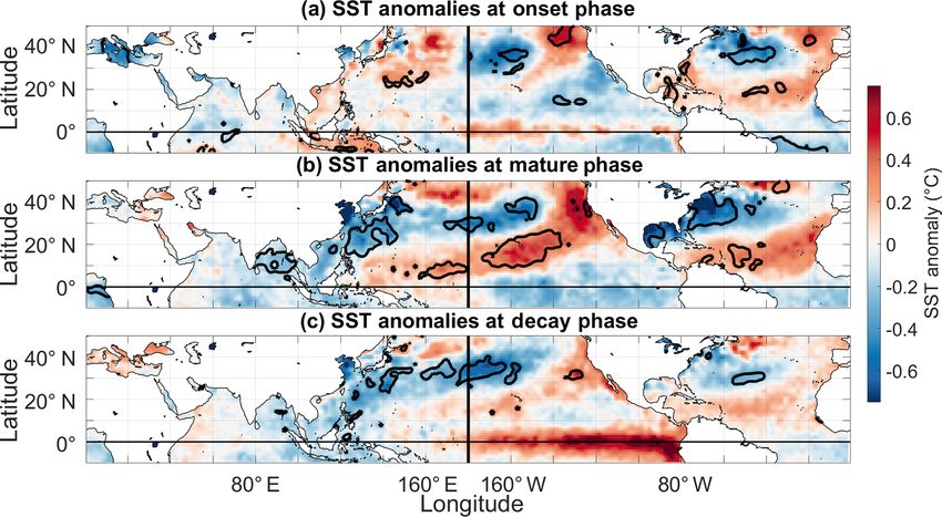
164                                                        J. A. Schulte and S. Lee: Long Island Sound temperature variability

Figure 1. (a) The 344 US climate divisions and (b) the LIS study region. Gray shading delineates the region used to calculate the LIS surface
water temperature time series.

tocorrelation coefficient measure of persistence needs to be             wavelet scale (Grinsted et al., 2004). Using Monte Carlo
calculated using a data interval so that the lag-1 autocorrela-          methods, the statistical significance of wavelet squared co-
tion coefficient may not reflect the persistence of an individ-          herence was assessed by generating 10 000 pairs of surrogate
ual event. A third advantage is that potential nonlinearities            red-noise time series with the same lag-1 autocorrelation co-
are accounted for by analyzing negative and positive events              efficients as the input time series and computing the wavelet
separately.                                                              squared coherence between each pair (Grinsted et al., 2004).
                                                                            To reduce the number of false positive results arising from
3.2   Wavelet analysis                                                   the simultaneous testing of multiple hypotheses (Maraun and
                                                                         Kurths, 2004; Maraun et al., 2007; Schulte et al., 2015;
To extract time-frequency information from a time series X,              Schulte, 2016), the cumulative area-wise test developed by
a wavelet analysis (Torrence and Compo, 1998) was imple-                 Schulte (2016) was applied. The test tracked how the ar-
mented. The wavelet transform of X is given by                           eas of contiguous regions of point-wise significance (signif-
          r       N
                              "         #
                                  0 − n δt                               icance patches) changed as the point-wise significance level
             2δt X              n
WnX (s) =             xn0 ψ ∗              ,             (2)             was altered. The test was applied by computing the normal-
              s n0 =1                s                                   ized areas of point-wise significance patches over a discrete
                                                                         set of point-wise significance levels. The normalized area of
where ψ is the Morlet wavelet given by
                                                                         a patch was defined as the patch area divided by the square of
                         1 2                                             its centroid’s scale coordinate (Schulte et al., 2015; Schulte,
ψ (η) = π −1/4 eiω0 η e− 2 η ,                                  (3)
                                                                         2016). In this study, the normalized areas were computed us-
where ω0 = 6 is the dimensionless frequency, t is time, s is             ing point-wise significance levels ranging from α = 0.02 to
wavelet scale, δt is a time step (1 month in this study), η =            α = 0.18. The spacing between adjacent point-wise signifi-
s·t, and the asterisk denotes the complex conjugate (Torrence            cance levels was set to 0.02.
and Compo, 1998).                                                           The strength of coherence was also measured using global
   To quantify the relationships between climate modes and               coherence (Schulte et al., 2016), the time-averaged represen-
water temperature as a function of frequency and time, a                 tation of local wavelet squared coherence. Global coherence
wavelet coherence analysis was conducted. Following Grin-                is given by
sted et al. (2004), the (local) wavelet squared coherence be-
tween two time series X and Y is given by                                                                       2
                                                                                              W XY (s)
                                                                         GC (s) =                              ,                       (5)
                                                                                       N
                                    2                                                             N
  2                  S s −1 WnXY (s)                                                   P  X
                                                                                         Wn (s)
                                                                                                2    P  Y
                                                                                                       Wn (s)
                                                                                                              2
Rn (s) =                                     ,         (4)                        n=1                 n=1
                           2                  2
          S s −1 WnX (s) · S s −1 WnY (s)
                                                                         where
where WnXY (s) is the cross-wavelet transform defined as the
product of the wavelet transform of X and the complex con-                            N
jugate of the wavelet transform of Y . In Eq. (4), S is a
                                                                                      X
                                                                         W XY (s) =         WnX (s)WnY ∗ (s).                            (6)
smoothing operator that smooths coherence in time and in                              n=1

Ocean Sci., 15, 161–178, 2019                                                                           www.ocean-sci.net/15/161/2019/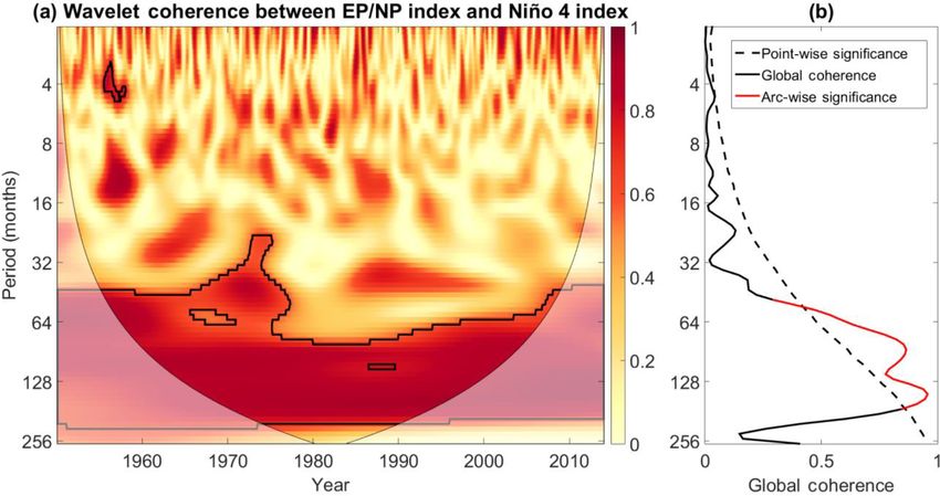
J. A. Schulte and S. Lee: Long Island Sound temperature variability                                                                 165

                                                                        Table 1. A total of 10 LIS detrended temperature events ranked by
                                                                        the magnitude of their intensities.

                                                                            Intensity   Persistence   Peak       Onset      Decay
                                                                                (◦ C)     (months)
                                                                                 20             13    Mar 2012   Oct 2011   Oct 2012
                                                                                −13             14    Jan 1982   Aug 1981   Sep 1982
                                                                                 13             15    May 1991   Dec1990    Feb 1992
                                                                                −13             12    Feb 2003   Nov 2002   Oct 2003
                                                                                −12             14    Jan 1996   Nov 1995   Dec 1996
                                                                                 11              6    Dec 2001   Nov 2001   Apr 2002
                                                                                 10              7    Jan 1983   Oct 1982   Apr 1983
                                                                                  9             14    Feb 1998   Dec 1998   Jan 2000
                                                                                 −8              8    Jan 2011   Sep 2010   Apr 2011
                                                                                 −8              5    Jan 1981   Nov 1980   Mar 1981

Figure 2. (a) The LIS surface temperature anomaly time series
                                                                        4     Results
and (b) the corresponding event spectrum. Central Pacific El Niño
events are indicated by CP and eastern Pacific El Niño events are in-   4.1    LIS temperature time series
dicated by EP. Blue curves represent the five most intense negative
LIS temperature events, while red curves represent the five most        The time series of detrended LIS temperature anomalies is
intense positive LIS temperature events. The length of the line         shown in Fig. 2a. Some notable features are the cool periods
segments in (b) represents the persistence of the LIS temperature       around 1982, 1996, and 2003 (thick blue lines) and the warm
events. The vertical axis corresponds to the intensity of the event.    events around 1991, 2001, and 2012. The 1982 cool period is
                                                                        rather intense, with LIS temperature anomalies approaching
                                                                        −2 ◦ C. In contrast, the 2012 event is associated with a max-
(Schulte et al., 2016). The statistical point-wise significance
                                                                        imum temperature anomaly of approximately 3 ◦ C, making
of GC (s) was computed using Monte Carlo methods in a
                                                                        this water temperature anomaly the largest in the 1979–2013
similar manner to local wavelet squared coherence.
                                                                        period.
   A lower-dimensional version of the cumulative area-wise
                                                                           Unlike the simple time series shown in Fig. 2a, the event
test was applied to the global coherence spectra to reduce the
                                                                        spectrum shown in Fig. 2b clearly distinguishes the intense
number of false positive results (Schulte et al., 2018). The
                                                                        LIS events from the weak short-lived events. For example,
test assessed the statistical significance of one-dimensional
                                                                        both the cool period around 1982 and the warm episode
arcs using arc length, which is an integrated metric account-
                                                                        around 2012 emerge as the most intense cool and warm
ing for the width of the peak in wavelet scale (frequency)
                                                                        events in the 1979–2013 period. The 1996, 2003, and 2011
and the extent to which the peak is above the critical level
                                                                        cold events are nearly as intense as the 1982 event (Table 1).
of the point-wise test. To track how the arc length of a given
                                                                        It is interesting to note that the most intense negative events
point-wise significance peak changed as the point-wise sig-
                                                                        shown in Table 1 peak in winter (December–February). This
nificance level was altered, the arc length of the point-wise
                                                                        tendency for negative events to peak in winter was confirmed
significance peak was computed at point-wise significance
                                                                        by computing the number of times a negative event peaked
levels ranging from 0.02 to 0.18. The test statistic in this case
                                                                        in a given month for a larger set of events (32 events) whose
is cumulative arc length. Normalized arc lengths were used
                                                                        intensities fall below the median of all negative event inten-
to account for how peaks widen with wavelet scale. This nor-
                                                                        sities. A similar but weaker tendency was found for positive
malization was achieved by computing the logarithm (base 2)
                                                                        events, with a majority of the most intense (greater than 50th
of the wavelet scales. To further normalize, global coherence
                                                                        percentile) positive events peaking in January and February.
values at each wavelet scale were divided by the critical level
                                                                           The event spectrum also allows for the clear comparison
of the test associated with the point-wise significance level
                                                                        of event persistence. An inspection of Fig. 2b shows that the
0.02 at each wavelet scale. The null distribution for the cu-
                                                                        intense events are generally more persistent than less intense
mulative arc-wise test was obtained by generating surrogate
                                                                        events. In fact, Table 1 shows that all the most intense events
red-noise time series in the same manner as the cumulative
                                                                        have persistence of at least 5 months, exceeding the average
area-wise test. For reference, we also plotted the traditional
                                                                        persistence of 3 months calculated using all events. Negative
5 % point-wise significance bounds on all global spectra plots
                                                                        and positive events were found to have similar average per-
in this study. The reader is referred to Schulte et al. (2018) for
                                                                        sistence. Given that the average persistence is 3 months, the
more details regarding the cumulative arc-wise test.
                                                                        1982, 1991, 1996, 2003, and 2012 LIS temperature events

www.ocean-sci.net/15/161/2019/                                                                           Ocean Sci., 15, 161–178, 2019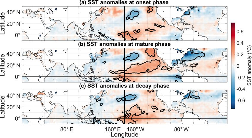
166                                                     J. A. Schulte and S. Lee: Long Island Sound temperature variability

are unusually persistent compared to other events in the study     ture extremes across the northeast US (Konrad, 1996, 1998).
period. Moreover, not only is the 2012 event among the most        Such surface anticyclones have been shown to be dynami-
persistent, but also its magnitude far exceeds that of any other   cally supported by a ridge–trough wave pattern in the mid-
event even with the removal of the long-term trend. This           dle troposphere (Konrad, 1998; Jones and Cohen, 2011), in
result suggests that atmospheric variability may have con-         agreement with the results shown in Fig. 3a. At the surface,
tributed strongly to that event.                                   the anticyclone results in cold advection from a high-latitude
                                                                   source region into the LIS region (Fig. 5a). Cyclones are also
4.2   LIS events and atmospheric patterns                          typically present along the east coast of the US during cold
                                                                   temperature events (Konrad, 1998), which could explain the
To diagnose a possible mechanism behind the occurrence             positive correlation between LIS temperature anomalies and
of the intense LIS events, the correlation between 500 hPa         SLP anomalies along the east coast of the US. Features as-
geopotential height anomalies and detrended LIS tempera-           sociated with positive LIS temperature anomalies are oppo-
ture anomalies was computed. We used this one-point cor-           site to those found for negative LIS temperature anomalies
relation approach to extract a relevant teleconnection pattern     (Fig. 5b).
from a continuum of patterns, much like how the PNA pat-              As a specific example, consider the SLP anomaly pattern
tern was originally derived (Wallace and Gutzler, 1981). For       for March 2012 (Fig. 4b). Negative SLP anomalies are seen
this analysis, we focused on the December–February (DJF)           to extend from western Alaska to central Canada, indicative
season because atmospheric circulation anomalies are gener-        of anomalously strong cyclonic flow and warm air advec-
ally most pronounced during the DJF season and because the         tion across the eastern US. The locations of the negative SLP
peak of events tends to occur in the winter.                       anomalies generally coincide where SLP anomalies are cor-
   Shown in Fig. 3a is the correlation between DJF LIS tem-        related with LIS temperature anomalies (Fig. 3b), again sug-
perature anomalies and 500 hPa geopotential height anoma-          gesting that the ridge–trough pattern played an important role
lies. The positive correlation between LIS temperature             in the March 2012 LIS temperature event.
anomalies and 500 hPa geopotential height anomalies over              To better understand LIS water temperature variability, a
the eastern US suggests that warmer-than-normal LIS tem-           ridge–trough dipole index was created based on the pattern
perature conditions are associated with a jet stream ridge,        identified in Fig. 3a. The dipole index was constructed by
which is consistent with how jet stream configurations can         first locating the grid point for which the correlation between
influence the temperature in the coastal ocean off the north-      LIS temperature and 500 hPa geopotential height anomalies
eastern US (Chen et al., 2014). Similarly, the negative cor-       is minimum. This grid point is located at 70◦ N and 157.5◦ W
relations with 500 hPa geopotential height anomalies across        and is marked by a cyan cross in Fig. 3a. Next, the grid
Alaska indicate that LIS warm events are associated with an        point for which the correlation between LIS temperature and
anomalous trough over Alaska. Thus, it appears that LIS tem-       500 hPa geopotential height anomalies is maximum was lo-
perature events are related to a ridge–trough dipole pattern,      cated. This grid point is located at 42.5◦ N and 75◦ W and is
an anomalously amplified wave pattern across the US.               marked with a magenta cross in Fig. 3a. Following Wang
   For comparison, the 500 hPa geopotential height anomaly         et al. (2014), the dipole index for a given month was de-
field for the March 2012 event is shown in Fig. 4a. Nega-          fined as the 500 hPa geopotential height anomaly at 42.5◦ N
tive 500 hPa geopotential height anomalies are seen across         and 75◦ W minus the 500 hPa geopotential height anomaly
Alaska, and positive 500 hPa geopotential height anomalies         at 70◦ N and 157.5◦ W. Thus, the dipole index measures the
are seen across the eastern US and across the central North        intensity of the ridge–trough dipole pattern such that positive
Pacific. This 500 hPa geopotential height anomaly configura-       phases generally indicate that an anomalously strong ridge
tion is consistent with the results presented in Fig. 3a, sug-     over the eastern US is accompanied by an anomalous trough
gesting that the ridge–trough dipole pattern was an important      over Alaska. Correlating the dipole index with SLP anoma-
contributor to the March 2012 LIS temperature event.               lies (not shown) reveals that negative (positive) phases of
   A physical mechanism behind the ridge–trough dipole–            the dipole pattern are associated with positive (negative) SLP
LIS temperature association was diagnosed by examining the         anomalies across northwestern Canada and cold (warm) air
relationship between DJF SLP anomalies and LIS tempera-            advection to the east of the anomaly center (Fig. 5).
ture anomalies. As shown in Fig. 3b, DJF LIS temperature              The time series for the 3-month running mean of the dipole
anomalies are negatively correlated with DJF SLP anoma-            index is shown in Fig. 6. The time series is rather noisy, but
lies across northwestern Canada. Thus, positive LIS tem-           notable features can still be identified. The dipole pattern,
perature anomalies are associated with anomalous cyclonic          as indicated by positive dipole indices, is seen to be in a
flow, whereas negative LIS temperature anomalies are asso-         persistent positive phase around the 2012 LIS warm event.
ciated with anomalous anticyclonic flow. These relationships       The positive dipole event around 2012 is quite intense but
are physically consistent with findings from previous works        not as intense as the 1882 positive dipole event that persists
showing how upstream (relative to the LIS) surface anticy-         for 11 months (Table 2). The most intense negative dipole
clones play a crucial role in the occurrence of cold tempera-      event occurs around 1977. A comparison of Tables 1 and 2

Ocean Sci., 15, 161–178, 2019                                                                  www.ocean-sci.net/15/161/2019/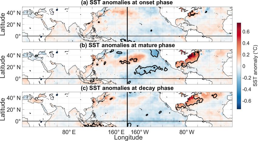
J. A. Schulte and S. Lee: Long Island Sound temperature variability                                                                  167

Figure 3. Correlation between LIS temperature anomalies and anomalies for (a) DJF 500 hPa geopotential height, (b) SLP, and (c) SST.
Contours enclose regions of 5 % statistical significance. Crosses in (a) mark the grid point locations used to construct the dipole index.

Table 2. A total of 10 dipole events in the 1851–2013 period ranked       Although a comparison of Tables 1 and 2 shows that the
by the magnitude of their intensities. Results are based on the raw    2012 LIS warm event coincides with the third most intense
monthly dipole index time series.                                      positive dipole event, the relationship strength between LIS
                                                                       temperature anomalies and the dipole pattern cannot be in-
  Intensity   Persistence   Peak         Onset        Decay            ferred. How strongly related is the dipole index to LIS water
       (m)      (months)                                               temperature anomalies? To assess the strength of the dipole
      847             11    Feb 1882     May 1881     Mar 1882         index relationship with LIS water temperature anomalies,
      844              9    Jan 1880     Oct 1879     Jun 1880         seasonally averaged detrended LIS temperature anomalies
      805              9    Mar 2012     Jul 2011     Mar 2012         were correlated with the seasonally averaged dipole index.
     −687              8    Jan 1977     Jul 1976     Feb 1977         As shown in Fig. 7, the dipole index is strongly correlated
     −666              9    Jan 2003     Oct 2002     Jun 2003
                                                                       with LIS temperature anomalies for the October–December
     −638              6    Jan 1978     Dec 1977     May 1978
     −616              7    Sep 1876     Jul 1876     Jan 1877
                                                                       (OND), November–January (NDJ), DJF, and January–March
     −604             12    Aug 1927     May 1927     Apr 1928         (JFM) seasons. The relationships are generally stronger if the
      580              6    Jan 1863     Dec 1862     May 1863         dipole index leads by 1 month, as indicated by the dotted
      572              9    Dec 1889     Nov 1889     Jul 1890         line in Fig. 7. The lagged correlation coefficients approach
                                                                       0.8 for the DJF season, suggesting that DJF LIS temperature
                                                                       anomalies are strongly influenced by the dipole pattern in
shows that the second most intense negative dipole event cal-          the NDJ season. Lagged correlations are also strong (r>0.6)
culated using the raw monthly dipole index time series co-             for the OND, NDJ, and JFM seasons. The relationships are
incides with the second most intense LIS cold event that oc-           generally weaker in the warm seasons, possibly because tele-
curred around 2003 (Table 1).                                          connection patterns are generally of the weakest amplitude
                                                                       in the warm season. Another reason is that LIS temperature

www.ocean-sci.net/15/161/2019/                                                                         Ocean Sci., 15, 161–178, 2019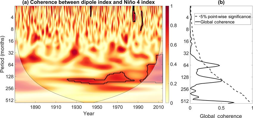
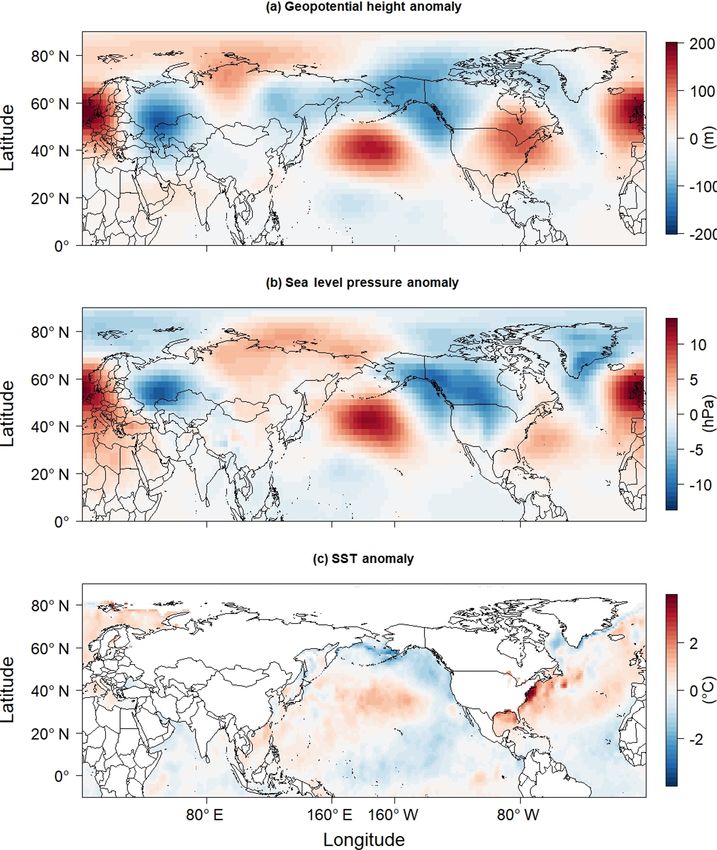
168                                                      J. A. Schulte and S. Lee: Long Island Sound temperature variability

Figure 4. Anomalies for (a) 500 hPa geopotential height, (b) SLP, and (c) SST corresponding to the March 2012 LIS temperature event.

anomalies in the winter can persist into the summer (Schulte          and peaks in January. With a such clear seasonal cycle, it is
et al., 2018), weakening the simultaneous relationships be-           natural to infer that the December dipole pattern is largely
tween LIS temperature anomalies and the dipole pattern for            the December EP–NP pattern despite how the CPC sug-
non-winter seasons. However, the weaker relationships be-             gests that the EP–NP pattern is inactive in winter. Because
tween air temperature and the dipole index in the summer              the 500 hPa geopotential height anomaly structure associated
(not shown) likely contribute to the seasonal cycle in rela-          with the dipole pattern is the same from November to March
tionship strength shown in Fig. 7.                                    (not shown), one can deduce that the December ridge–trough
   The relationship strength found between the dipole in-             pattern is largely the December EP–NP pattern given the
dex and LIS temperature anomalies is consistent with results          strong relationship between EP–NP and dipole indices dur-
found in prior work because the dipole index is strongly cor-         ing those months. More specifically, we compared the De-
related with the EP–NP index for most months (Table 3)                cember dipole pattern to the January dipole pattern (Fig. 8)
and because the EP–NP index is strongly correlated with               and found them to be similar in terms of 500 hPa geopoten-
LIS temperature anomalies (Schulte et al., 2018). However,            tial height anomalies. Thus, because the January dipole and
Schulte et al. (2018) used an ad hoc approach to construct            EP–NP indices are strongly correlated, the December dipole
the December EP–NP index using linear regression. Thus,               pattern must also be EP–NP-like. The strong relationships
one may ask the following: is the EP–NP pattern a winter-             (r>0.8) between air temperature and the dipole pattern in
time pattern? To answer the question, it is first noted that          winter suggest that the dipole pattern (or EP–NP pattern) is
the relationship strength between the EP–NP and dipole in-            particularly active in the winter. It also has a strong physical
dices increases nearly monotonically from August to Novem-            basis because negative phases are associated with 500 hPa
ber, decreases almost monotonically from January to August,           western North America and Arctic ridging and eastern US

Ocean Sci., 15, 161–178, 2019                                                                      www.ocean-sci.net/15/161/2019/
J. A. Schulte and S. Lee: Long Island Sound temperature variability 169
Table 3. Correlation between the dipole index and indices for five major climate modes of variability for the 1979–2013 period. Bold entries
indicate 5 % statistically significant correlation coefficients.
J F M A M J J A S O N D
EPNP 0.74 0.67 0.67 0.66 0.56 0.52 0.47 0.26 0.43 0.66 0.66 –
WP −0.28 −0.34 −0.19 −0.37 0.21 0.34 0.42 0.33 0.00 −0.31 −0.6 −0.56
PNA 0.29 0.0 0.0 0.0 0.35 0.12 0.12 0.46 0.43 0.30 0.15 0.0
AO −0.6 −0.18 −0.49 −0.21 −0.52 −0.40 −0.45 −0.40 −0.37 −0.65 −0.58 −0.62
NAO −0.59 −0.15 −0.53 −0.13 −0.50 −0.40 −0.18 −0.13 −0.1 −0.55 −0.46 −0.59
pattern’s eastern center of action (magenta cross in Fig. 3a)
but are practically uncorrelated with 500 hPa geopotential
height anomalies around the western center of action. The
NAO and AO are also much more strongly correlated with
500 hPa geopotential height anomalies across the North At-
lantic than the dipole pattern. The WP index is only weakly
correlated with 500 hPa geopotential height around both the
dipole patterns’ centers of actions and much more strongly
correlated with 500 hPa geopotential height anomalies across
the western North Pacific Ocean. Our results suggest that the
reason why the wintertime AO, NAO, and WP patterns are
not strongly related with wintertime LIS temperature anoma-
lies as shown by Schulte et al. (2018) is that these patterns are
not related to northern Alaskan jet stream ridging, which is
important to LIS temperature variability (Fig. 3a).
The fact that the dipole index is correlated with multiple
large-scale indices (Table 3) suggests that the dipole pattern
falls on a continuum of teleconnection patterns (Franzke and
Feldstein, 2005) such that the dipole pattern is strongly EP–
NP-like. Although we found by conducting our own EOF
analysis of 500 hPa geopotential height anomalies that the
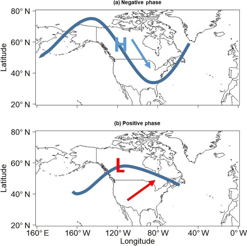
Figure 5. (a) Idealized schematic of atmospheric features occur- AO pattern is the leading mode of variability, the EP–NP
ring during negative LIS temperature events and negative phases of pattern appears to be consistently the fifth to seventh lead-
the dipole pattern. (b) Same as (a) but for positive LIS temperature ing mode of variability (Table 4). Thus, although the EP–NP
events and positive phases of the dipole pattern. Thick blue curves pattern is not as dominant as the AO pattern, the dipole pat-
represent the idealized jet stream configuration, while the blue (red) tern tends to more closely resemble it than the AO pattern.
arrow indicates the general movement of cold (warm) air masses. Furthermore, the continuum-based extraction of a dipole pat-
High pressure is indicated with an H and low pressure is indicated
tern with a strong relationship to LIS temperature anomalies
with an L.
supports the idea that the continuum approach is useful for
understanding climate variability across the northeast US, a
finding like that described in previous work focusing on pre-
500 hPa troughing (Fig. 8), all features associated with east- cipitation in the northeast US (Schulte et al. 2017a, b). In par-
ern US cold temperature events (Konrad, 1998). Although ticular, our results show that the one-point correlation map
Schulte et al. (2018) used the EP–NP index to diagnose his- approach used by Wallace and Gutzler (1981) is a powerful
torical LIS temperature variability, our dipole index is de- but simple tool for understanding regional climate variability.
fined in all months and is easy to calculate, making it more Given that LIS water temperature is strongly correlated
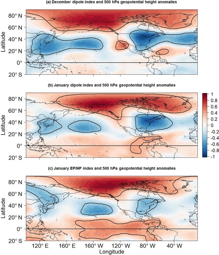
practical in an operational forecasting setting. with air temperature (Schulte et al., 2018), it is hypothesized
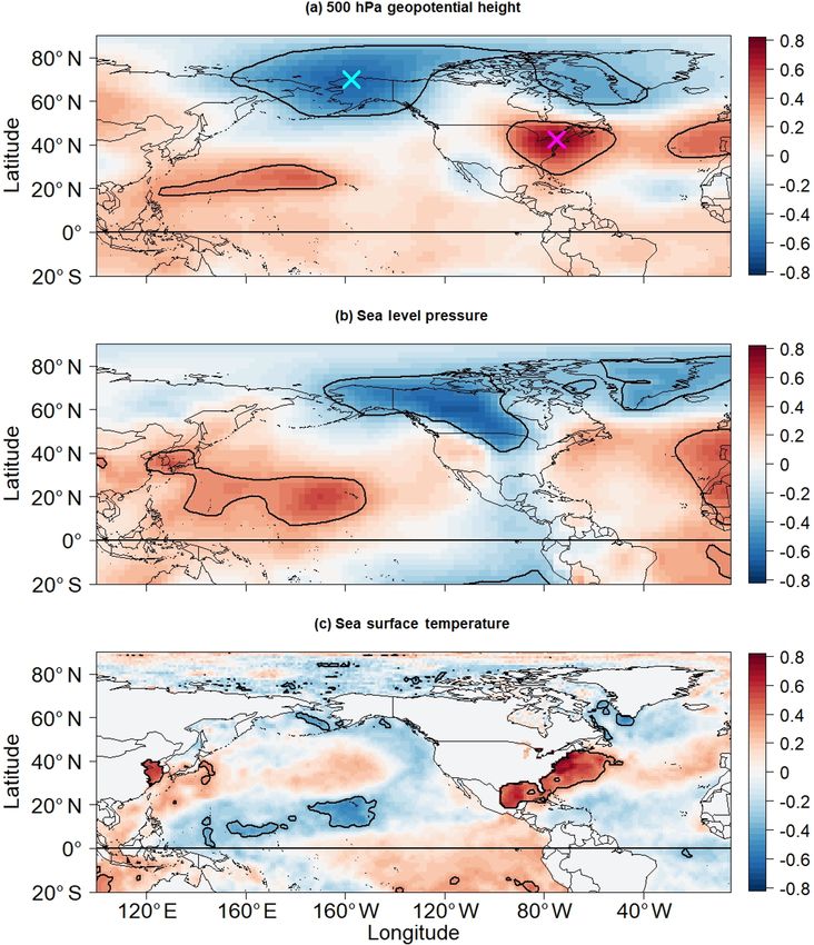
While the December dipole index is well correlated with that the dipole index is related to air temperature across the
December indices for the AO, NAO, and WP, a close ex- US, especially around the LIS. To confirm a dipole index–
amination of the 500 hPa geopotential height anomaly fields air temperature relationship, the dipole index was corre-
(not shown) associated with those patterns reveals that those lated with average monthly air temperature anomalies for the
patterns are quite different from the dipole pattern found in 1979–2013 period (Fig. 9). The results for the NDJ season
this study. For example, the NAO and AO indices are cor- are only displayed because the strongest correlation found in
related with 500 hPa geopotential height around the dipole
www.ocean-sci.net/15/161/2019/ Ocean Sci., 15, 161–178, 2019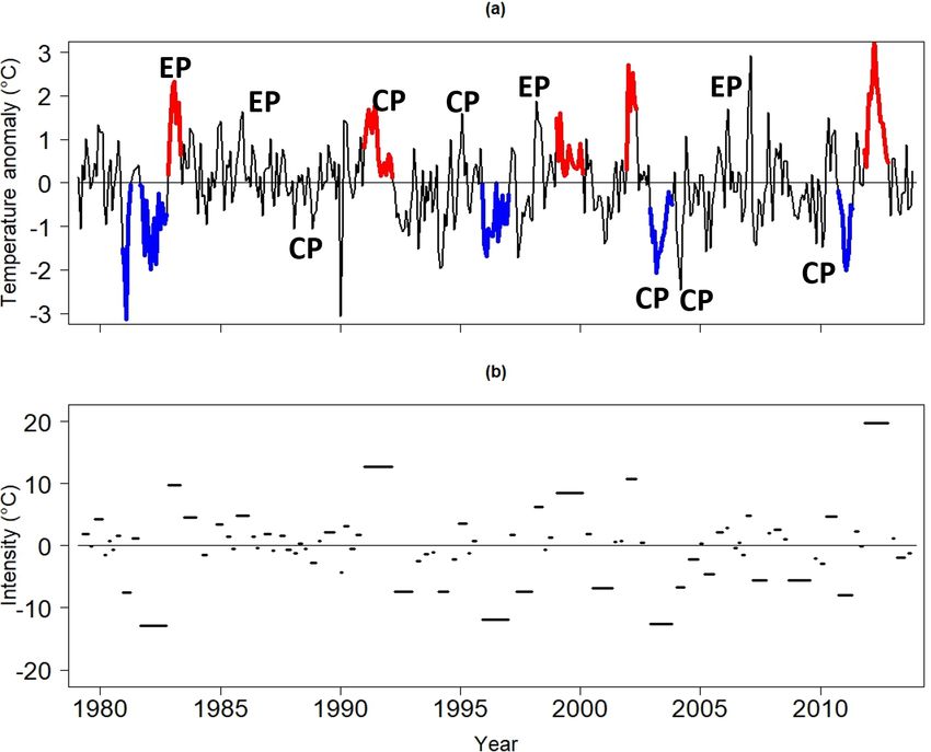
170                                                       J. A. Schulte and S. Lee: Long Island Sound temperature variability

Figure 6. The 3-month running mean of the dipole index.

Figure 7. Lagged and simultaneous correlations between seasonally averaged LIS water temperature anomalies and the seasonally averaged
dipole index. The dotted line represents the correlation between the dipole index of the prior season (dipole leads by 1 month) and water
temperature anomalies for the season specified on the horizonal axis.

Fig. 7 is between the NDJ dipole index and DJF LIS water               in 2012 (Dole et al., 2014), which resulted in a so-called false
temperature anomalies.                                                 spring in which plants bloomed prematurely, making them
   As shown in Fig. 9, the dipole index is indeed strongly cor-        susceptible to drought and freezes (Ault, 2013). The results
related with air temperature anomalies across a large region           shown in Fig. 9 suggest that the dipole pattern’s impact on
of the US. Correlation coefficients exceed 0.8 and approach            LIS temperature is related to the dipole pattern’s influence
0.9 across the northeast US and LIS region. The strong re-             on air temperature.
lationships extend to the southern US, and the relationships
generally weaken equatorward. The relationships displayed              4.3   Intense LIS events and SST patterns
in Fig. 9 are generally stronger than those associated with
the AO and NAO (not shown) whose influence on eastern                  SST patterns are often used in seasonal forecasting, and
US temperature has been well studied (Hurrell and van Loon,            thus identifying an SST pattern precursor to LIS tempera-
1997; Wettstein and Mearns, 2002). Thus, our dipole index              ture events has implications for seasonal prediction of LIS
is useful for diagnostic studies of cold outbreaks across the          temperature anomalies. To identify SST patterns associated
eastern US. The results for the other seasons are similar, but         with LIS temperature events, a lagged SST composite analy-
the relationships for seasons not comprising November, De-             sis was conducted using detrended LIS warm and cool events
cember, January, or February (e.g., June–August) are gener-            separately. The SST composite plots for the warm events
ally weaker than those identified for the NDJ season. This re-         were constructed using the LIS warm events whose inten-
sult suggests that the dipole pattern is rather dominant in the        sities are greater than or equal to the 50th percentile of all
winter. The strong relationship between the dipole index and           warm event intensities (32 events). Similarly, the SST com-
US air temperature anomalies is consistent with the intense            posite plots for the cold events were constructed using LIS
2012 dipole event coinciding with the record warm March                cold events whose intensities are less than or equal to the
                                                                       50th percentile of all LIS cold event intensities (32 events).

Ocean Sci., 15, 161–178, 2019                                                                       www.ocean-sci.net/15/161/2019/
J. A. Schulte and S. Lee: Long Island Sound temperature variability 171
Figure 8. Correlation between 500 hPa geopotential height anomalies and indices for the (a) December dipole, (b) January dipole, and
(c) January EP–NP patterns. Contours enclose regions of 5 % statistical significance.
Table 4. The mode number of the EOF pattern that most closely resembles the EP–NP pattern, the explained variance associated with the
EOF pattern, and the correlation coefficient, r, computed between the corresponding principal component time series and the EP–NP index.
The EOF pattern that most closely resembles the EP–NP pattern was determined by finding the EOF pattern whose principal component time
series is most strongly correlated with the EP–NP index. The results are based on NCEP reanalysis for the 1979–2013 period.
Quantity J F M A M J J A S O N D
r 0.66 0.66 0.61 0.62 0.67 0.44 0.51 0.60 0.63 0.69 0.61 –
Variance (%) 14.4 5.5 3.2 5.0 7.0 1.9 4.3 5.2 4.7 6.0 4.4 –
EOF number 2.0 6.0 7.0 6.0 4.0 11.0 5.0 5.0 6.0 5.0 7.0 –
The composite mean SST patterns were computed at the on- 2005, and 2009–2010 events (Table 5), but a more complete
set, mature, and decay phases of the LIS events. Because in- list can be found in Johnson and Kosaka (2016). The 2002–
tense LIS events tend to peak in winter, the composite plots 2003, 2004–2005, and 2009–2010 events all appear to occur
for mature phases mainly reflect wintertime conditions. around LIS cold periods (Fig. 2a). Note that there could be
The results for the LIS cold events are shown in Fig. 10. lags between the onset of central Pacific El Niños and LIS
The composite plot shown in Fig. 10a indicates that the onset temperature anomalies because of the lagged response of wa-
of LIS cold events is associated with positive SST anomalies ter temperature to atmospheric forcing (Schulte et al., 2018).
across the central equatorial Pacific. The results suggest that In addition, preexisting positive water temperature anomalies
LIS cold events could be initiated by central Pacific El Niño may need time to degrade.
events (Lee and McPhaden, 2010). A few examples of cen- The SST anomaly pattern for the mature phases of LIS
tral Pacific El Niño events (based on the December–March cold events features positive SST anomalies across the cen-
season) are the 1991–1992, 1994–1995, 2002–2003, 2004– tral equatorial Pacific (Fig. 10b). However, the mature-phase
www.ocean-sci.net/15/161/2019/ Ocean Sci., 15, 161–178, 2019172 J. A. Schulte and S. Lee: Long Island Sound temperature variability
riod for much of the US (Halpert and Bell, 1997) and the LIS
(Table 1).
Unlike the composite mean SST pattern corresponding to
the onset phase, negative SST anomalies are present along
the US east coast and across the Gulf of Mexico during ma-
ture phases. These results are consistent with LIS tempera-
ture anomalies being strongly associated with the dipole pat-
tern that influences air temperature across regions adjacent to
the Gulf of Mexico and US east coast. This relationship be-
tween the dipole index and SST anomalies was confirmed by
correlating the dipole index with SST anomalies for different
seasons (not shown).
The tropical SST pattern associated with the decay phase
of LIS cold events is different from those associated with
Figure 9. Correlation between the NDJ dipole index and NDJ tem-
perature anomalies. Shaded climate divisions are those for which the onset and mature phases (Fig. 10c). The composite mean
the corresponding correlation coefficients are statistically signifi- SST anomaly pattern most closely resembles the first lead-
cant at the 5 % significance level. ing mode of SST variability called the canonical ENSO pat-
tern (Hartmann, 2015), though the most intense positive SST
anomalies are still confined to the central equatorial Pacific.
Table 5. El Niño events partitioned into central (CP) and eastern This result suggests that there may be a tendency for the de-
(EP) Pacific types based on the categorization method of Yu et cay of LIS cold events to coincide with canonical ENSO pat-
al. (2012). El Niño events are defined based on the DJFM season. terns or an SST pattern that is a mixture of central and eastern
The third column provides the corresponding DJFM LIS tempera- Pacific El Niño flavors lying on a continuum of ENSO flavors
ture anomaly. A more complete table of El Niño events can be found (Johnson, 2013).
in Johnson and Kosoka (2016).
The tendency for the decay of LIS cold events to coincide
with canonical ENSO patterns is more evident when con-
El Niño years Event LIS temperature
structing SST composites using the 10th percentile (Fig. 11)
type anomaly (◦ C)
instead of the 50th percentile used to construct the composite
1982–1983 EP 1.9 shown in Fig. 10. However, possibly because of small sam-
1986–1987 EP 0.2 ple sizes (seven events), the results generally lack statisti-
1987–1988 CP −0.2 cal significance. Nonetheless, the event spectrum depicted in
1991–1992 CP 0.3 Fig. 2b indicates that the major cool periods around 1982 and
1994–1995 CP 0.7
1997, for example, terminate around the major 1982–1983
1997–1998 EP 0.9
2002–2003 CP −1.5
(Ramusson and Wallace, 1983; Quiroz, 1983) and 1997–
2004–2005 CP −0.4 1998 (McPhaden, 1999) El Niño events. Although Schulte
2006–2007 EP 0.7 et al. (2018) showed that LIS temperature anomalies are as-
2009–2010 CP −0.6 sociated with a single SST pattern, we show in this study
that predicting the evolution of LIS temperature events may
require knowledge of several ENSO flavors.
The SST pattern across the Atlantic Ocean shown in
composite mean SST anomaly pattern is more pronounced Fig. 11 resembles a well-documented North Atlantic tripole
across the North Pacific Ocean than it is for the onset phase. mode (Deser and Blackmon, 1993; Fan and Schneider,
A region of positive SST anomalies is seen to be horseshoe- 2011), which comprises three anomaly centers, one located
shaped, with positive SST anomalies extending from the cen- off the southeastern US coast, a second one located east of
tral equatorial Pacific to the US west coast. Although Hart- Newfoundland, and a third one located in the tropical east
mann (2015) found an SST pattern resembling that shown in Atlantic. This tripolar SST mode has been shown to be re-
Fig. 9b to be a contributor to the February 2015 eastern US lated to ENSO, the NAO, and local wind forcing (Fan and
cold event, only a single event was considered. In this study, Schneider, 2011). The association between the tripole pattern
we show that the pattern is associated with numerous LIS and the LIS water temperature could reflect weak influences
negative temperature events (and thus eastern US air temper- of the NAO on LIS water temperature. This interpretation is
ature events), many of which persist for more than 5 months. consistent with the NAO and dipole patterns being related in
Thus, we show here that the SST pattern influences both the the winter (Table 3). However, these Atlantic SST anomalies
intensity and persistence of events. It is noted that the pattern generally lack statistical significance, and this finding is con-
shown in Fig. 10b resembles the DJF SST pattern of 1996, sistent with the LIS water temperature anomalies being only
which is consistent with 1996 being a cooler-than-normal pe- weakly related to the NAO.
Ocean Sci., 15, 161–178, 2019 www.ocean-sci.net/15/161/2019/J. A. Schulte and S. Lee: Long Island Sound temperature variability 173 Figure 10. Composite mean SST anomalies corresponding to (a) onset, (b) mature, and (c) decay phases of negative LIS temperature events. Contours enclose regions of 5 % statistical significance, as determined by a one sample t test. Figure 11. Same as Fig. 10 but using the criterion that the intensities of the negative LIS temperature events fall below the 10th percentile of negative LIS temperature event intensities. The composite analysis was also conducted for LIS warm tern associated with March 2012 (Fig. 4c), a month in which events, and the results revealed that LIS warm events are also record warmth was experienced across the central and east- associated with SST modes of variability (Fig. 12). The on- ern US (Dole et al., 2014). Mature phases are also associ- set of LIS warm events appears not to be associated with any ated with positive SST anomalies along the US east coast and coherent SST pattern. For the mature phase, statistically sig- across the Gulf of Mexico like March 2012 (Fig. 4c). Decay nificant negative SST anomalies are seen across the central phases (Fig. 12c) appear to be associated with negative SST equatorial Pacific and positive SST anomalies are seen across anomalies across the eastern and central equatorial Pacific, the eastern equatorial Pacific. Like the SST anomaly pattern but the results were not found to be statistically significant. associated with mature phases of LIS cold events (Figs. 10b The warm LIS events were found to be sensitive to the and 11b), the pattern shown in Fig. 12b generally resembles threshold used to construct the composites. For example, the third leading mode of SST variability (Hartman, 2015). if we only considered the LIS warm events whose intensi- The SST pattern corresponds well to the SST anomaly pat- ties were greater than or equal to the 90th percentile of LIS www.ocean-sci.net/15/161/2019/ Ocean Sci., 15, 161–178, 2019
174                                                       J. A. Schulte and S. Lee: Long Island Sound temperature variability

Figure 12. Same as Fig. 10 but for positive LIS temperature events.

warm event intensities, then all phases of LIS warm events               The results shown in Fig. 13a indicate that the dipole and
would resemble the pattern shown in Fig. 12b. In general,             Niño 4 indices fluctuate coherently in the 64- to 256-month
the positive SST anomalies across the eastern Pacific were            period after 1930. The results suggest that stronger decadal-
found to become more intense as the percentile used to es-            scale fluctuations in central equatorial Pacific SSTs are as-
tablish the threshold was increased from 50 to 90. Despite            sociated with larger decadal fluctuations in the dipole pat-
the lack of statistical significance in the composite plots, sta-     tern. Given that the decadal-scale fluctuations in the dipole
tistically significant relationships with SST anomalies were          pattern contribute to the overall variance of the dipole index
found when correlating DJF LIS temperature anomalies with             around 2012, the decadal-scale fluctuations must contribute
DJF SST anomalies (Fig. 3c). The identified correlation pat-          to some extent to the intense dipole event of 2012. The re-
tern was found to resemble the pattern shown in Figs. 10b             sults from the coherence analysis thus suggest that central
and 11b.                                                              equatorial Pacific SST fluctuations may have contributed to
   The SST composite analyses were also conducted using               that intense dipole event.
the dipole events for the 1979–2013, 1950–2013, and 1870–                The strong correlation between the EP–NP and dipole in-
2013 periods. The resulting SST patterns were found to be             dices (Table 3) suggests that the coherence between the EP–
like those shown in Figs. 10, 11, and 12, which is not sur-           NP and Niño 4 indices is also strong. The strong coherence
prising given the strong correlation between the dipole in-           was confirmed by computing the wavelet squared coherence
dex and LIS temperature anomalies. Thus, intense long-lived           between the EP–NP and Niño 4 indices for the 1950–2013
dipole patterns seem to have a tropical origin, suggesting that       period. To perform the analysis, the missing values for the
a key to better understanding LIS temperature events rests in         EP–NP index in December were filled by establishing a lin-
a firmer understanding of tropical processes.                         ear relationship between the EP–NP and dipole indices for all
                                                                      months but December. The linear relationship was obtained
4.4   Decadal variability                                             using a least-squares fit of a line, and it was used to fill miss-
                                                                      ing EP–NP values based on the available December dipole
The results of the composite analyses suggest that dipole             index values.
events may be associated with tropical SST patterns, but the             As shown in Fig. 14, the EP–NP index does indeed fluc-
timescale at which the SST patterns are most strongly as-             tuate coherently with the Niño 4 index. The coherence ap-
sociated with the dipole pattern cannot be inferred from the          pears to be strong, and the global coherence spectrum shows
analysis. Thus, a wavelet coherence analysis was conducted            arc-wise significant global wavelet coherence in the 64–256
to determine if the SST modes fluctuate coherently with the           month period. As shown by Schulte et al. (2018), the EP–
dipole pattern at a preferred timescale. The wavelet squared          NP pattern fluctuates strongly on quasi-decadal timescales,
coherence was computed between the dipole index and in-               but no possible source of the variability was identified. We
dices for the Niño 3 and Niño 4 metrics, but the results using        show in Fig. 14 that the EP–NP variability on quasi-decadal
the Niño 4 index were found to be most robust. As such, the           timescales may be related to quasi-decadal fluctuations in
results for the Niño 4 index analysis only are shown.                 central equatorial Pacific SSTs. Because the EP–NP pat-

Ocean Sci., 15, 161–178, 2019                                                                      www.ocean-sci.net/15/161/2019/
You can also read