Bitcoin's Crypto Flow Network - arXiv
←
→
Page content transcription
If your browser does not render page correctly, please read the page content below
Bitcoin’s Crypto Flow Network
                                           Yoshi Fujiwara1 and Rubaiyat Islam1
arXiv:2106.11446v2 [q-fin.GN] 6 Jul 2021

                                           1
                                               Graduate School of Information Science, University of Hyogo, Kobe 650-0047, Japan
                                           E-mail: yoshi.fujiwara@gmail.com
                                           (Received May 31, 2021)

                                           How crypto flows among Bitcoin users is an important question for understanding the structure and
                                           dynamics of the cryptoasset at a global scale. We compiled all the blockchain data of Bitcoin from
                                           its genesis to the year 2020, identified users from anonymous addresses of wallets, and constructed
                                           monthly snapshots of networks by focusing on regular users as big players. We apply the methods of
                                           bow-tie structure and Hodge decomposition in order to locate the users in the upstream, downstream,
                                           and core of the entire crypto flow. Additionally, we reveal principal components hidden in the flow
                                           by using non-negative matrix factorization, which we interprete as a probabilistic model. We show
                                           that the model is equivalent to a probabilistic latent semantic analysis in natural language processing,
                                           enabling us to estimate the number of such hidden components. Moreover, we find that the bow-tie
                                           structure and the principal components are quite stable among those big players. This study can be a
                                           solid basis on which one can further investigate the temporal change of crypto flow, entry and exit of
                                           big players, and so forth.
                                           Presented at the conference “Blockchain in Kyoto 2021”, and forthcoming in the JPS Conference
                                           Proceedings.
                                           KEYWORDS: Bitcoin, cryptoasset, bow-tie structure, Hodge decomposition, non-negative
                                           matrix factorization, latent Dirichet allocation, complex network

                                           1. Introduction

                                                Cryptoasset or cryptocurrency is essentially a digital ledger to record transactions between cred-
                                           itors and debtors, just like money. The digital system is based on a collection of non-centralized
                                           ledgers, called blockchain, which contains all the historical record of transactions among anonymous
                                           users. Today there are many cryptoassets being exchanged in markets with fiat currencies and also
                                           with each other. The market capitalization is so huge in total ranging from one to a few trillion USD,
                                           and highly volatile potentially having a big impact even on asset markets and prices of non-crypto at
                                           a global scale.
                                                In this paper, we study Bitcoin, the largest one dominating nearly half of the market capitalization
                                           at the time of writing. We attempt to understand the flow of crypto as a complex network comprising
                                           of the users as nodes and the crypto flow as links. There are a number of studies from such a viewpoint
                                           of complex network on cryptoassets. See [1–16] for example, and references therein.
                                                Specifically, in this paper, we focus on “big players” who are defined as persistently appearing
                                           users, likely to be involved in transactions of high frequencies and large amounts, and address the
                                           following questions. First, it is important to identify the users in the upstream, downstream, or core in
                                           the entire crypto flow. We shall examine the so-called “bow-tie” structure of the network of those big
                                           players to classify the location of the crypto flow based on the binary relationship of links. Second, we
                                           measure the location in a more quantitative way by using the information of flow along the links in the
                                           combinatorial method of Hodge decomposition. Third question is to extract “principal components”
                                           hidden in the entire crypto flow so as to uncover a certain number of latent factors or components.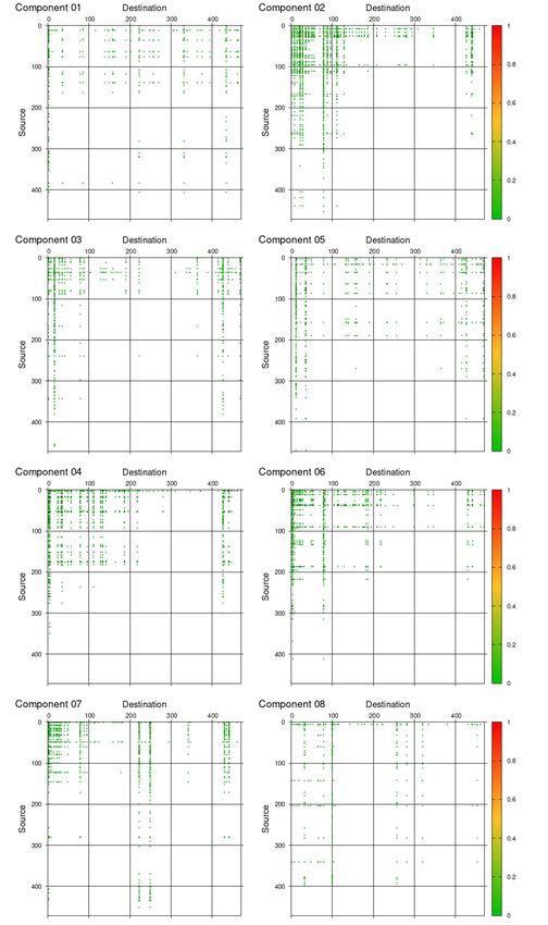
Fourth, because the network is changing in time, what can one say about the stability of the crypto
flow?
    In Section 2, we describe our dataset of Bitcoin to identify the anonymous addresses representing
wallets into users. Then we define regular users as big players and construct networks. In Section 3.1,
we perform the bow-tie analysis to locate users in the stream of crypto flow. In Section 3.2, we use the
method of Hodge decomposition to quantify the location of users. In Section 3.3, we introduce non-
negative matrix factorization as a method of matrix decomposition to reveal principal components
hidden in the flow. We shall show in Section 3.4 that the method can be interpreted as a probabilistic
model, from which one can estimate the number of components. In Section 3.5, we find about a dozen
of principal components among several hundred big players, and show that the temporal change of
the network is quite stable. In Section 4, we discuss about several aspects, being worth further investi-
gation, and conclude in Section 5. We add Appendix A for the identities (actual names, business, and
so forth) of selected users. Appendix B illustrates the networks in adjacency matrices. Appendix C
briefly summarizes the above mentioned probabilistic model in relation to latent Dirichlet allocation,
from which the estimation on the number of components is done in Appendix D.

2. Data

    We employ the dataset of all transactions recorded in the Bitcoin blockchain from the genesis
block (first block issued on January 9, 2009) until the block of height 63,299 (inclusive; issued on
June 4, 2020). Each transaction is a transfer of a certain amount of BTC (monetary unit of Bitcoin)
from one or more addresses to others as we will see shortly. We call such a transfer of BTC as crypto
flow. An address is something like a wallet possessed by a user who can be an individual or, more
frequently today, an agent in the business of exchanges, services, gambling, and so forth.
    In the dataset, total number of transactions was 1.38 billion, while the number of different ad-
dresses was about 657 million. To study crypto flow of Bitcoin, one needs to know users, rather than
the addresses. However, it is not straightforward to identify users from addresses because of the very
nature of anonymity inherent in the core technology of blockchain. See [17] for technical details.
    Let us employ a simple but useful method to identify users from addresses to construct a giant
graph comprising of nodes as users and edges as crypto flow. We shall see that more than 60% of the
addresses can be identified with users. Additionally we will see that a number of users can be revealed
with their actual names, types of business, and sometimes geographical location at a global scale.
Then we define regular users as big players in order to focus on a subgraph comprising of frequently
appearing users who are involved in crypto flow with huge amounts of BTC. The subgraph will be
studied in the subsequent sections.

2.1 Identification of Users from Addresses
   Consider an example of such a transaction (TX) that one day Alice transferred 1 BTC to Bob:

                                      TX1 : {a1 , a2 } → {a123 , a1 } ,                                (1)

where the addresses a1 and a2 belong to Alice, while a123 belongs to Bob. Alice needs more than
one address as input of TX1 , because a single one was not sufficient to fulfill the amount of 1 BTC.
Output of TX1 includes a1 representing the change. Another day, Alice did another transaction:

                                       TX2 : {a1 , a3 } → {a45 , a3 } ,                                (2)

where the address a3 also belongs to Alice. Obviously, multiple addresses, if and only if they appear
in an input of a transaction, belong to the same user, namely her wallets. As a consequence from both
of (1) and (2), it follows that a1 , a2 , a3 can be identified to belong to the same user. Note that a2 and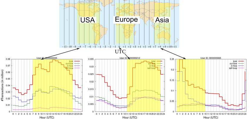
Fig. 1. Rank-size plot for the number of addresses identified with users. Size (horizontal) is the number of
addresses identified with users of type A (a group of addresses appearing in multiple inputs of transactions, so
identified as user; see main text). Rank (vertical) is the descending order of the size. Maximum size is nearly
20 million, while minimum is 2 and average is 6.7.

a3 did not appear in any record of transactions, TX1 and TX2 . By looking at all the transaction in the
history, one can identify many addresses with users.
     This simple but useful method to identify users from addresses was proposed by [1] and has been
extensively used in the literature (see [4, 5] and the data of [18, 19], for example). We implemented
an efficient algorithm of this method to process the above mentioned 657 million addresses in the
1.375 billion transactions. We found that 402 million addresses (more than 60%) can be identified
to obtain 60 million different users (denoted as type A). The rest of 255 million addresses, which
never appeared as multiple inputs in any transactions, are regarded as different users (type B). This
procedure results in 315 million users all together.
     Fig. 1 shows a rank-size plot, in which the size is the number of addresses identified with users
of type A, and the rank is its descending order. The minimum size is 2 by construction, while the
average is 6.7. It is interesting to observe that the rank-size plot is highly skewed with the maxi-
mum size being nearly 20 million! We labeled all the users of type A in a sequential user ID cor-
responding to the rank (e.g. 0000012345), while users of type B is labeled with its address (e.g.
3CjqmbuRA1LEWmLHiWoSWHcWuTEVPfU24P).
     A bunch of transactions is packed into a block in the blockchain. Each block has a timestamp
of its birth, which is UTC (Coordinated Universal Time) when the block was mined or born as an
empty ledger to be filled with transactions. We associate the time with the transactions contained in
the block. Each block is mined in a mean time of 20 minutes or longer, as is well known, so it should
be understood that by time we mean a rough estimate on when the transaction was made within an
accuracy of an hour or so. One can use this information of the timestamp to obtain the intra-day
activities of users. Fig. 2 is a schematic diagram for typical three users, presumably located in Asia,
Europe including Africa, and USA.
     Moreover, with the help of laborious investigation by [19], it is possible to unravel the identity
of users of type A with actual names, types of business, and sometimes geographical location for
many users. Appendix A is the summary of the unraveled identity. Table A·1 gives the classification
of business into exchanges, gambling, pools, services and others. Nearly one third in the list are
exchanges. Table A·2 is the list of countries of those exchanges, where China, UK, and USA are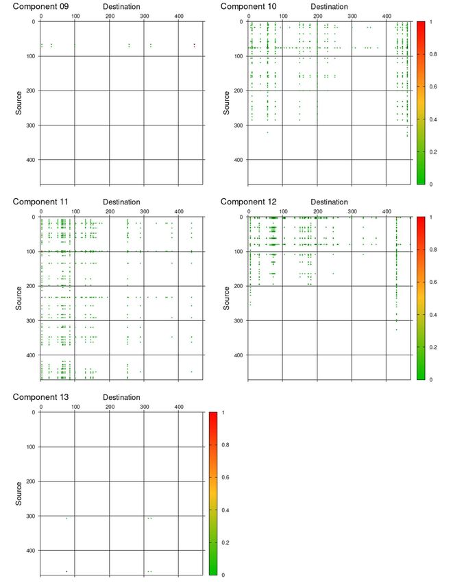
Fig. 2. Schematic diagram for the intra-day activities of users. Top is a world map with UTC (Coordinated
Universal Time). The bottom three plots depict the number of transactions involving three users. Each plot
shows the numbers of transactions of out-flow (green), in-flow (blue), self-loop (magenta), and their total (bold
red), where each number is accumulated during the year 2019. Out-flow, in-flow, and self-loop are respectively
the transaction in which the user is its source, destination, and both of them simultaneously. A peak of the red
line shows the most active time, corresponding to the daytime of USA, Europe, and Asia (left to right). Arrows
indicate noon of specific locations.

dominant, followed by Canada, Australia, Brazil, Singapore, and Russia. In fact, as found in the
top of Table A·3, the user ID 0000000000 corresponding to the maximum size in Fig. 1 is actually
Bit-x.com and Xapo.com, the former of which is an agent of exchange in South Africa.
     Exchanges are a typical category of “big players” in the sense that they actually hold a huge
number of individuals and agents as customers resulting in a large number of transfers. As a matter
of fact, the daily number of transfers has an interesting weekly pattern. There is significantly less
activity in weekends than in weekdays as found in recent data of Bitcoin1 (see our previous study
[21, 22]). Such a weekly pattern implies that those institutional agents are dominant in the entire flow
of crypto.

2.2 Crypto Flow Network
    Now all the transactions among addresses are converted into transfers from users to users, each
of which has the following information:
   • user of source s,
   • user of destination d,
   • amount of Bitcoin transferred from s to d, i.e. s → d,
   • UTC time of transfer (from the block containing the transaction).
    During a certain period of time T , for a pair of users, there can be more than one transfer as
depicted in Fig. 3 (see the left-hand side). In this example, there are three transfer of crypto for i → j,
one for j → i, and also two for i → i. The last case of self-loop is possible, because one can receive a
change in a transaction, and also because different addresses are possibly identified with a user, like

   1
     Cryptoasset of XRP has a similar weekly pattern according to [20]. In the early history of Bitcoin, the weekly pattern
was quite the opposite; more active in weekends, presumably because individuals were big players at that time.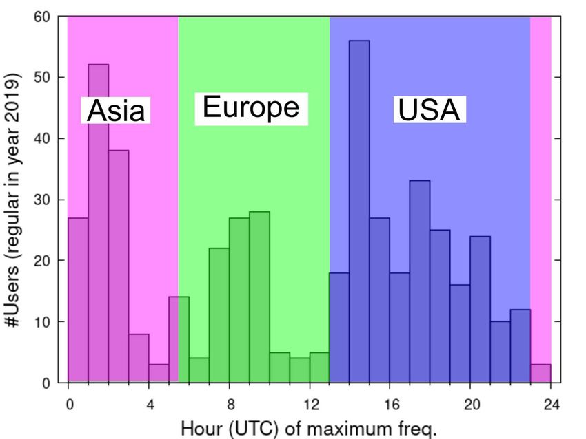
0.1                                             fij = 0.7
                1
                            0.2                                              gij = 3
                                                Aggregated
                                                                    i                        j
                 i          0.4           j
                                                                            fji = 0.1
                                                                 fii = 3     gji = 1
                2           0.1
                                                                 gii = 2

Fig. 3. Aggregation of transactions to construct crypto flow network. Left: During a given period of time,
for a pair of users i and j, three transfers for i → j with 0.1, 0.2, 0.4 in BTC, one of j → i with 0.1, and two
for i → i with 1 and 2. Right: After aggregation, one has i → j with frequency fi j = 3 and amount of flow
gi j = 0.7. Similarly, j → i with f ji = 1 and amount of flow g ji = 0.1, and i → i with fii = 2 and gii = 3.

an exchange. Given a time-scale T , it would be reasonable to aggregate these transactions as shown
in the right-hand side of Fig. 3.
     After the aggregation, one has a network comprising of nodes as users and edges with direction
given by the transfer of crypto, frequency and amount of transfer occurred during the period of time.
Let us denote the following variables which represent the strength or weight of each edge by
                    frequency fi j ≡ frequency of transfers for i → j,
                    amount of flow gi j ≡ amount of total transfers for i → j.
     Regarding the time-scale T for aggregating the transactions and the epoch to select in the histor-
ical data, we choose one month and the calendar year of 2019. By examining the time-series for the
daily number and amount of transactions, we assumed that the period of one month is adequate to
study the stability and temporal change of the crypto flow. Shorter period may lead to a trivial result
for the stability and could be insufficient to detect the temporal change, if any change is present. Also
longer period would be misleading due to non-equilibrium nature of the system. The year 2019 was
chosen as the epoch, in which one does not see violent bubble or crush in the price.
     The number of all the users is huge, 315 million users in total. Fortunately, however, it is not
necessary to include all of them, because most of them do not appear frequently. In the next section,
we shall extract only a tiny part of the network by focusing on the “regular users” who appeared
everyday during the specified period.

2.3 Regular Users as Big Players
     For our purpose in this paper, it is sufficient to focus on the crypto flow with high frequency and
big amount of Bitcoin, because infrequent and/or small amount of flows is obviously unimportant
for the understanding the entire flow. In other words, it suffices to focus on “big players” who are
playing some dominant role in the game of crypto flow. It would be possible to define such a big
player in different ways. In this study, we define it by looking at how persistently the user appears in
transactions during our specified period of time.
     Fig. 4 depicts examples of users who appear in different numbers of transactions on daily basis.
The user of the top case is persistent in committing transactions with other users, which can be labeled
as a “regular user”. The middle case changes the persistency from being inactive with no transaction
with anyone else to being active in an abrupt way. The bottom case has little activity, just a few
transactions on particular days having a strong intermittency.
     We define regular users as those appearing everyday during the period of one year in 2019, and
use them as big players. The number of regular users was 479. Then we construct a subgraph in each
month, which is comprised of the regular users as nodes and the crypto flow as links, the latter of
which are aggregated as described in Fig. 3. Thus we have 12 snapshots of such subgraphs, each
Fig. 4. Illustrative examples for the activities of users. Each plot depicts the daily number of transactions,
in each of which the user is either source or destination of the transaction for the period of year 2019. Self-
loops (case of the same source and destination) are excluded. Top is a “regular” user appearing every day. The
middle user became active from being inactive, while the bottom one has intermittency in its activity. We focus
on regular users in this paper.

Fig. 5. Activities of regular users, defined by each user’s peak of transactions, in UTC. Shaded region corre-
sponds to the daytime of Asia, Europe, and USA (left to right).

corresponding to each month in the year, from January to December. Summarizing the processing of
the whole dataset, we constructed the snapshots of networks denoted by Gt = (Vt , Et ), where t is the
month, Vt is the set of regular users, Et is the set of links among them, each having the frequency and
amount as depicted in Fig. 3.
    We add Fig. 5 showing the histogram for the UTC time of highest activities of all the regular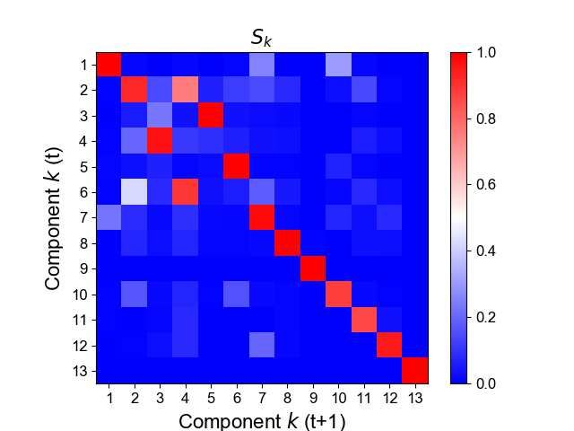
users in the year of 2019. This information gives geographical locations of those regular users.
3. Analysis of Crypto Flow Network
3.1 Basic Properties of Network
For each month t, we constructed a network denoted by Gt = (Vt , Et ) as described in the preceding
section. Table I is the summary of basic properties of the networks in the year 2019. Vt corresponds
to the regular users in each month, the number of which is shown by the column |Vt |. The column
|Et | is the number of edges, namely the number of different crypto flow from one user to another or
to itself (self-loops as shown in parentheses). Most of the users have self-loops. Temporal change of
the network causes the changes of Vt and Et . The column of |Vt ∩ Vt+1 | is the number of users that are
common to successive months in their appearance. One can see that most of the users are appearing
successively. The same is true for the edges as shown in the column of |Et ∩ Et+1 |. In other words,
the network is not changing drastically in terms of the entry and exit of nodes and edges during the
time-scale of months.
Table I. Summary of basic properties of the networks in the year 2019, January to December.
t |Vt | |Et | |Vt ∩ Vt+1 | |Et ∩ Et+1 | GWCC GSCC/IN/OUT/TE
01 470 17,215(408) 468 13,313 468(3) 327/24/113/4
02 470 16,658(407) 468 13,357 468(3) 322/20/120/6
03 473 17,618(408) 471 13,942 470(4) 327/25/113/5
04 473 17,691(415) 470 13,960 469(5) 336/16/115/2
05 472 17,903(416) 471 14,012 468(5) 330/23/112/3
06 471 17,787(412) 469 13,705 467(5) 318/23/124/2
07 472 17,292(410) 468 13,108 470(3) 333/21/110/6
08 468 16,534(402) 467 12,628 466(3) 321/18/123/4
09 470 16,288(407) 468 12,652 466(5) 325/23/113/5
10 469 16,317(402) 468 12,476 467(3) 322/21/119/5
11 470 15,859(409) 466 12,080 468(3) 324/23/116/5
12 466 15,584(390) — — 466(1) 323/18/120/5
Each column represents the following.
t= month of the year 2019
|Vt |= number of nodes
|Et |= number of edges (number of self-loops in parentheses)
|Vt ∩ Vt+1 |= number of nodes common to successive months
|Et ∩ Et+1 |= number of edges common to successive months
GWCC= number of nodes in giant weakly connected component (number of components in parentheses)
GSCC/IN/OUT/TE= number of nodes in giant strongly connected component/IN/OUT/tendrills
We found that most of the users have self-loops, as shown in the parentheses of column |Et |,
with the frequencies fii and the amounts gii being highly correlated with the number of addresses
identified in the preceding Section 2.1 as naturally expected. Because our main interest in this paper
is the crypto flow from one user to another, we remove all the self-loops in what follows.
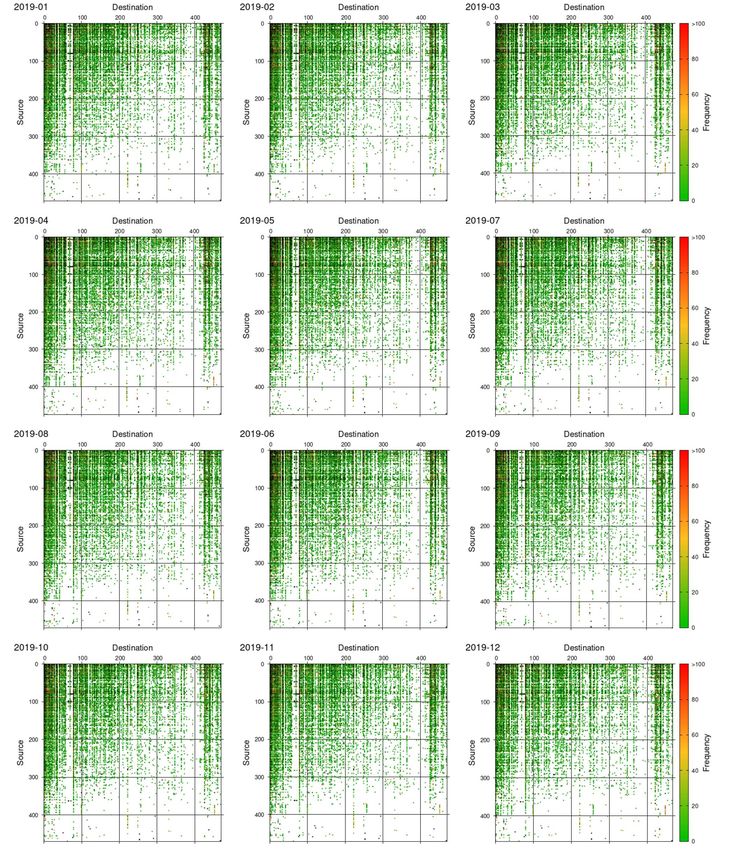
Adjacent matrices with the strength of links given by the frequencies fi j of Gt for all t’s are
illustrated in Appendix B. One can see that the overall picture does not change in time, but the
illustration does not help to uncover the nature of connectivity and flow.
To see the connectivity of network, namely how those regular users are linked among them and
also how they are located in the stream of cypto flow, let us examine the property of connected com-Fig. 6. Temporal change of bow-tie structure in an alluvial diagram. Monthly data of networks in the year
2019, January to December (from left to right). Vertical black segments in each month show the nodes of
corresponding network grouped into GSCC (giant strongly connected component), IN, OUT, and TE (tendrills)
in the bow-tie structure. Horizontal bands represent transitions among such groups from one month to its
successive one.
ponents. First, decompose Gt into weakly connected components (WCC), i.e. connected components
when regarded as an undirected graph. We found that there exists a giant WCC (GWCC) containing
most of the users. See the column GWCC of Table I. There was only a small number of disconnected
components as shown in the same column.
Then, in order to identify the location of users contained in the GWCC, we employed the well-
known analysis of “bow-tie” structure [23]. In general, GWCC can be decomposed into the following
parts:
GSCC Giant strongly connected component: the largest connected component when viewed as a
directed graph. One or more directed paths exist for an arbitrary pair of firms in the component.
IN The nodes from which the GSCC is reached via at least one directed path.
OUT The nodes that are reachable from the GSCC via at least one directed path.
TE “Tendrils”; the rest of the GWCC.
It follows that
GWCC = GSCC + IN + OUT + TE (3)
GSCC is the core of the crypto flow’s circulation. The IN and OUT parts are upstream and down-
stream of the flow respectively. The users in the part of IN are playing a role of suppliers of crypto,
while the OUT users are considered to be consumers of crypto.
Table I shows the bow-tie structure in the column of GSCC/IN/OUT/TE. For example, in Septem-
ber, 470 users are located into GSCC (325 users), IN (23), OUT (113), and TE (5). One can observe
that a large fraction of the users in the GWCC is located in the GSCC, as one can easily interpret this
fact in the way that those regular users are circulating crypto globally. There are a less fraction of the
users in IN and OUT with asymmetry in the numbers.
It would be interesting to see how the individual users are located in the temporal change of the
network. Fig. 6 depicts such a diagram of temporal change from one month to its successive one in the
whole year. One can see that the groups of GSCC, IN, and OUT are very stable in each membership
of users. This fact means that those users appearing in successive months are playing stable roles in
the crypto flow’s circulation and the location of upstream and downstream. We remark that analysisof bow-tie structure is based on the binary links, namely either presence or absence among the nodes,
but not on the strength of links such as frequency and amount of crypto flow. In the next section, we
shall see how to quantify the location of users by using the so-called Hodge decomposition.
3.2 Hodge Decomposition
Helmholtz-Hodge-Kodaira decomposition, or simply Hodge decomposition, is a combinatorial
method to decompose flow on a network into circulation and gradient flow. Original idea dates back
to the Helmholtz theorem in vector analysis, which states that under appropriate conditions any vector
field can be uniquely represented by the sum of an irrotational or rotation-free (curl-free) vector field
and a divergence-free (solenoidal) vector field. The theorem can be generalized from Euclidean space
to graph and other entity as shown by Hodge, Kodaira and others. See [24–26] for readable exposition.
The method has a wide range of applications in the studies such as neural network [27], economic
networks [28, 29], and also our previous work on Bitcoin and [30].
We recapitulate the method briefly for the present manuscript to be self-contained. Let Ai j denote
the adjacency matrix:
1 if there is a link of transfer from user i to j,
Ai j =
(4)
0 otherwise.
We excluded all the self-loops, implying that Aii = 0. Each link has a flow, denoted by F̃i j , either of
the frequency, fi j , or the amount, gi j , of the transfer from i to j (see Fig. 3). Define
fi j or gi j if Ai j = 1,
F̃i j = (5)
0 otherwise.
Note that there can be a pair of users such that Ai j = A ji = 1 and F̃i j , F̃ ji > 0.
Let us define a “net flow” Fi j by
Fi j = F̃i j − F̃ ji (6)
and a “net weight” wi j by
wi j = Ai j + A ji . (7)
Note that wi j is symmetric, i.e., wi j = w ji , and non-negative, i.e., wi j ≥ 0 for any pair of i and j2 .
Hodge decomposition is given by
(g)
Fi j = Fi(c)
j + Fi j , (8)
where the circular flow Fi(c)
j satisfies X
Fi(c)
j =0, (9)
j
(g)
which implies that the circular flow is divergence-free. The gradient flow Fi j can be expressed as
(g)
Fi j = wi j (φi − φ j ) . (10)
Thus the weight wi j serves to make the gradient flow possible only where a link exists. We refer to
the quantity φi as the Hodge potential. Large value of φi implies that the user i is in the upstream of
the entire network, while small values implies i is in the downstream.
2
It is remarked that (7) is simply a convention to consider the effect of mutual links between i and j. One could multiply
(7) by 0.5 or an arbitrary positive number, which does not change the result significantly for a large network.25
GSCC
IN
OUT
20
Frequency
15
10
5
0
-2 -1 0 1 2
Hodge potential
Fig. 7. Distributions for Hodge potentials of the users in GSCC (black), IN (blue), and OUT (red). The
average of all the potential values is set to be zero (vertical dotted line). Data: 2019-09.
Combine (8), (9), and (10), one can derive the following equation to determine φi .
X X
Li j φ j = Fi j , (11)
j j
for i = 1, . . . , N. Here, Li j is the so-called graph Laplacian and defined by
X
Li j = δi j wik − wi j , (12)
k
where δi j is the Kronecker delta.
It is easy to show that the matrix L = (Li j ) has only one zero mode (eigenvector with zero
eigenvalue). The presence of this zero mode simply corresponds to the arbitrariness in the origin of φ.
All the other eigenvalues are positive (see, e.g., [30]). Therefore, (11) can be solved for the potentials
by fixing the potentials’ origin. We assume that the average value of φ is zero.
Fig. 7 depicts the distributions for Hodge potentials of the users in GSCC, IN, and OUT. One can
see that the entire set of distributions is bimodal having two peaks at positive and negative values,
while there are a number of values around zero. Obviously, they correspond to IN, OUT, and GSCC,
each being located in the upstream, downstream, and core of the entire crypto flow. Moreover, there
exists a correlation between the value of the Hodge potential and the net amount of demand or supply
of crypto by each user. See [30] for details, where we studied a daily snapshot of the network including
all the users, not only big players. We claim that the same property holds also for the monthly data
restricted to big players of regular users.
3.3 Non-negative Matrix Factorization
It would be a natural question whether there are distinctive ingredients of flows in the crypto flow
or not. The analysis of bow-tie structure is based merely on the binary relationship of links, so does
not give such information, because the crypto flows from upstream to downstream with circulation in
the giant strongly connected component that occupies a large fraction of the entire network. In otherwords, are there any “principal components” that constitute the entire flow in a decomposition? In
order to find such principal components or latent factors in the transfer of crypto among big players,
we shall apply non-negative matrix factorization (NMF) to the strength of links, namely the matrix of
the frequencies and amounts of transfer. We recapitulate the method here. See [31–33] and references
therein for introduction.
Let X be an N × M non-negative matrix, in general, to start with; that is, its elements are all
non-negative, denoted as X ≥ 0. NMF gives an approximation of X by a product of two matrices:
X ≈ SD , (13)
where S , D are N × K and K × M non-negative matrices, S , D ≥ 0, respectively3 . In practice, one
expects that K is much smaller than N and M so that the factorization gives a compact representation
of X. We shall assume that N = M for our application of crypto flow among N users in what follows.
Explicitly in components, (13) reads
X
K
X sd ≈ S sk Dkd , (14)
k=1
where the indices s and d represent source and destination (s, d = 1, . . . , N) respectively, and X sd is
the strength of crypto flow, quantified by frequency f sd , amount gsd , or similar variables, from s to d
in a certain period of time. We choose
X sd = f sd , (15)
in this paper. See Fig. B·1 in Appendix B for the illustration of X sd . We would expect that K ≪ N,
because of the sparsity of X. How to determine K is discussed later.
The approximation in (13) is actually given by the following optimization:
min F(X, S D) , (16)
S ,D≥0
where the function F(·, ·) is the so-called Kullback-Leibler (KL) divergence defined by
X !
Ai j
F(A, B) = KL(AkB) ≡ Ai j log − Ai j + Bi j . (17)
i, j
Bi j
Note that F(A, B) = 0 if and only if A = B. The reason why we choose the particular function of
(17) will be clarified later4 . Technically, one can solve (16) iteratively with the initialization of S , D
using non-negative double singular value decomposition (see the review [32] and references therein).
Although the iterative algorithm yields local minima, our numerical solutions under different random
seeds gave essentially the same decomposition.
To understand the meaning of the decomposition, let us consider how a source distributes flow to
different destinations. For an arbitrary source s, (14) can be written as
X
K
Xs ≈ S sk Dk , (18)
k=1
where X s is the vector of s-th row of X, and Dk is the vector of k-th row of D. Equation (18) means
that the flow from the source s can be expanded in terms of “basis” vectors, Dk (k = 1, . . . , K). The
3
The decomposition is not unique due to trivial degrees of freedom. One is permutation, S D = S ππ−1 D, where π is
a permutation matrix simply exchanging indices. Another is scale transformation, S D = S σσ−1 D, where σ is a diagonal
matrix with all elements positive. We shall see that these degrees are fixed after appropriate normalization and ordering.
4
See Section 3.4 for a probabilistic interpretation of choosing the KL divergence. Another functional form, often used,
P
is the so-called Frobenius norm: F(A, B) = (1/2) i, j (Ai j − Bi j)2 , which leads to a different probabilistic model.components (Dk )d = Dkd represent how destinations are distributed among users in the k-th NMF
component. It is convenient to normalize Dk by L1-norm, that is, by defining
X
ekd ≡ Dkd where Dk ≡
D Dkd , (19)
Dk d
so that one has X
ekd = 1 ,
D (20)
d
for all k. With respect to this normalized basis vectors, the expansion in (18) is rewritten as
X
K
Xs ≈ ek
(S sk Dk )D where e k )d = D
(D ekd , (21)
k=1
Thus the outgoing flow from the source s is approximately expressed by a linear combination of K
normalized basis vectors De k with coefficients given by S sk Dk .
Similarly, consider how a destination d collects flow from different sources. For an arbitrary
destination d, (14) reads
XK
Xd ≈ Dkd Sk , (22)
k=1
where Xd is the vector of d-th column of X, and Sk is the vector of k-th column of S . The components
of (Sk )s = S sk represent how sources are distributed among users in this k-th NMF component. Define
S sk X
Sesk ≡ where S k ≡ S sk , (23)
Sk s
and one has X
Sesk = 1 , (24)
s
for all k. Then (22) is rewritten as
X
K
Xd ≈ ek
(Dkd S k )S where ek ) s = Sesk .
(S (25)
k=1
Thus the incoming flow to the destination d is approximately expressed by a linear combination of K
normalized basis vectors S ek with coefficients given by Dkd S k .
How can one determine K? Obviously, the larger K is, the better the approximation (13) is, but
with less parsimonious representation of the data. In the next section, let us make a detour to examine
this issue from a different perspective.
3.4 NMF as a probabilistic model
We can interpret the NMF as a probabilistic model. Denote the right-hand of (14) by
X
ξ sd ≡ S sk Dkd , (26)
k
which are regarded as parameters to be estimated from the data X such that X sd is assumed to be a
random number chosen from a Poisson distribution with the parameter ξ sd as
ξx
P(x | ξ) = e−ξ . (27)
x!It is easy to see that the log likelihood function L(ξ sd ) ≡ log P(X sd | ξ sd ) takes the maximum value at
ξ sd = X sd . Then one can introduce a quantity to measure how much the estimation of the parameters
is good, that is !
X X X sd
(L(X sd ) − L(ξ sd )) = X sd log − X sd + ξ sd , (28)
s,d s,d
ξ sd
to be minimized. One can see that this quantity is equivalent to the KL divergence in (17)5 .
To express the entire framework in probabilistic terms more explicitly, let us normalize the data
X in (15) by
esd = P X sd
X . (29)
s′ ,d′ X s′ d′
Then let us rewrite (14) as X
esd ≈
X rk Sesk D
ekd , (30)
k
ekd and Sesk were given by (19) and (23) respectively, and
where D
S k Dk
rk ≡ P , (31)
k ′ S k ′ Dk ′
P
which satisfies that k rk = 1. Let us denote the right-hand side of (30) by
X
psd ≡ rk Sesk D
ekd , (32)
k
P
which satisfies that s,d psd = 1. We remark that the normalized weight rk defined by (31) gives
the information of relative importance of the k-th NMF component in the expansion with normalized
basis vectors in (32). One can determine the ordering of NMF components uniquely according to the
magnitudes of rk .
Suppose that there are N f transfers in total during a period of time. For each pair of source and
destination, s and d, generate a transfer s → d with the probability given by psd , being independently
of other pairs. Under the assumption of a small probability of psd and a large number of N f , X sd
follows a Poisson distribution with the parameter, ξ sd = N f psd .
It turns out that the decomposition in (26), or equivalently (32), has an interesting connection
with machine learning. In natural language processing, it is often necessary to extract topics among
documents comprising of words or terms. In a situation of unsupervised learning, the task is to infer
topics as hidden or latent variables, which can explain a collection of documents, each being an
unordered set of terms. Probabilistic latent semantic analysis (PLSA) is a probabilistic model for
doing such a task [36]. Suppose that there are N documents and M terms. Then the occurrence of
terms can be expressed by a document-term matrix X with size N × M, each element of which is the
frequency of occurrence of a term in a document. Topics are latent variables to explain the data X. A
topic is actually a probability distribution for the occurrence of terms with different probabilities. A
document can have a mixture of topics. An example is a document on “influence of hosting Olympics
to economy” with a mixture of topics on sports and economy.
One of the widely used model of PLSA is latent Dirichlet allocation (LDA). See Appendix C and
references therein. For our purpose, it suffices to understand how terms are generated at locations of
documents in a probabilistic way. The probability that a term is chosen at a location in a document is
given by the sum of K factors, each of which is the product of two probabilities; the probability that
5
We became aware that this argument is known in the literature. If one assumes Gaussian instead of Poisson, one would
have Frobenius norm for KL divergence in (17). See [34]. One of the present authors (YF) learned a hint on the argument
from Itsuki Noda in his application of NMF to transportation data [35].1 45
99% interval
avgerage (20 simulations)
40
LDA score (in arbitray units)
Measure (to be minimized)
0.8
35
30
0.6
25
20
0.4
15
10
0.2
CaoJuan (2009) 5
Arun (2010)
Deveaud (2014)
0 0
0 10 20 30 40 50 0 10 20 30 40 50
#Components #Components
(a) Comparison of three methods [38–40] (b) Monte Carlo simulations by the method [39]
Fig. 8. Determining K, the number of NMF components, by using the concept of coherence in LDA. (a) Dif-
ferent methods [38–40] are compared. Each measure of coherence is drawn in the vertical axis so that it is to
be minimized to find the optimal number of components. Maximum and minimum values in the region of K
are scaled to 1 and 0 respectively to make the comparison easier. One can see that K = 11 ∼ 13 are optimal.
(b) Monte Carlo simulations by the method [39] with 20 runs for each K. Averages (points) and 99% level
(gray band, narrow) calculated from standard errors are drawn. We conclude that K = 13 is optimal from this
result (b).
a topic is selected in the document and the one that the term is chosen under the selected topic. See
the equation of (C·11) in Appendix C. One can immediately see that (C·11) is essentially the same
as (26), or equivalently (32).
Thus the matrix decomposition of NMF can be put in the framework of probabilistic model of
PLSA and LDA. As a bonus, one can adopt the method of estimating the number of topics to our
problem of determining the number of NMF components, denoted by K in both cases. Interested
readers are guided to look at the literature [37–40] and others given at the end of Appendix C. Let us
take a look at our results in the next section finishing the detour of this section.
3.5 Result of NMF for Crypto Flow
We first show a few results for a snapshot of September in the year 2019 (denoted as 2019-
09), in order to verify if the idea in the preceding section works to determine the number of NMF
components. Fig. 8 shows the measures of coherence by employing three different methods of LDA
[38–40]. The methods give mostly the same optimal values of K, namely K = 11 ∼ 13, consistently
as shown in Fig. 8 (a). We found that the measure given in [39] is relatively stable and potentially
useful to determine a specific value of K. So we performed Monte Carlo simulations in Fig. 8 (b), and
were able to determine the optimal value as K = 13. For this data, X has the dimension of N = 470,
so we conclude that one can have a small number of NMF components that can explain the entire
flow among those regular users.
In Appendix D, we summarize the same result for the data in all the other months of the year
2019. We found that the optimal number K is quite small in the range more than 10 and less than 20,
much smaller than the number of users, N ∼ 500 (see Table I). Additionally, K is relatively stable
irrespectively of the temporal change. See Table D·1 and Fig. D·1.
Let us examine each NMF components obtained with the optimal value of K. Fig. 9 and Fig. 10
show the NMF components in terms of the basis vectors, D e k and S
ek , respectively for k = 1, . . . , K.
e
In Fig. 9, each plot shows the vector components of (Dk )d = Dkd meaning how destinations are
distributed among users d in the k-th NMF component. Similarly in Fig. 10, each plot shows thevector components of (S ek )s = S sk meaning how sources are distributed among users s in the k-
th NMF component. See (19) and (23), and also note the normalization therein. Note that in each of
Fig. 9 and Fig. 10, the plots are ordered (from top to bottom) in the descending order of the probability
rk given in (31).
One can immediately notice from the figures that the components of these basis vectors are con-
centrated on a limited number of users, but are not distributed among many users. To quantify the
effective number of the concentration, let us use the inverse Herfindahl-Hirschman index, abbrevi-
ated as IHH, which is defined as follows. Consider “shares” xi ≥ 0 among i = 1, . . . , N things with
P
the sum equal to 1, i.e. i xi = 1. The IHH is defined by
N −1
X
IHH ≡ x2i . (33)
i=1
When the shares are equal, xi = 1/N for all i, then IHH = N. On the other hand, when there is the
strongest concentration, namely, xi = 1 for a particular i and xi = 0 otherwise, then IHH = 1. So
IHH can give an estimate of the effective number of large shares6 . The idea can be applied to the
basis vectors, because the vectors are normalized in the same way as shares. In Fig. 9 and Fig. 10, we
displayed all the calculated IHH’s. One can see that the IHH’s are quite small ranging from a few to
a dozen or so, compared with the total number of users N = 470 for the data 2019-09 (see Table I).
How can we use the NMF components to understand the crypto flow? Choose a particular user s
as a source s. The flow from s was approximately expressed by a linear combination of K normalized
basis vectors De k , each depicted in Fig. 9, with the coefficients given in (21), i.e. S sk Dk . The coeffi-
cients represent the strength of the decomposed flow from the source s. A similar argument holds by
choosing a particular user d as a destination. The flow to d was expressed by a linear combination in
(25) with the coefficients, Dkd S k .
For example, consider the user with ID 0000000000 that is located in the GSCC, as a source s.
Fig. 11 shows the coefficients corresponding to K components; see (a). One can see that the coeffi-
cients are non-zero at only four components. Such a sparseness tells that the flow from this user can
be expressed with a few components. And the corresponding components have non-zero values at a
small number (recall the IHH’s) of the vector components, Dkd , as shown in Fig. 9, implying that the
users corresponding to these non-zero components constitute a cluster for the outgoing flow from the
source s.
The same user 0000000000 can be regarded as a destination d in the GSCC. Fig. 11 (b) shows
the coefficients, again non-zeros at only one or two components. Together with Fig. 10, one can
find another cluster composed of a small number of users for the incoming flow to the d. Similar
arguments hold for the users 0000006178 and 0000000012, respectively located in the IN and OUT.
See Fig. 11 (c) and (d). In this way, one can find clusters for either of or both of the outgoing and
incoming flows of each user.
Each NMF component can be represented by a matrix, because the non-negative matrix of X sd
or its probabilistic counter part psd can be expressed by (18) or (32). It is possible to depict each
component k by the matrix of Sesk D ekd in the normalized way. Fig. 12 and Fig. 13 illustrate such
matrices for the data of 2019-09. This should be compared with X sd in Appendix B. One can see that
the NMF components provide sparse matrices.
Finally, we find that the NMF components are relatively stable in the temporal change of network.
Fig. 14 (a) shows the result for cosine similarities of the NMF basis vectors Dk for the two successive
months of 2019-09 and 2019-10. Fig. 14 (b) shows the result for Sk for the same data. In either of
these results, one can see that the NMF components are quite similar except only a few permutation
of indices.
6
It is remarked that the paper [20] in this volume also applied but modifies Herfindahl-Hirschman index in an interesting
way to characterize the frequencies of transactions in XRP.Destination (user index)
0 100 200 300 400
k= 1: Prob=27.3%, IHH= 5
0.25
0
k= 2: Prob=13.8%, IHH=35
0
0.25 k= 3: Prob= 9.3%, IHH=10
0
k= 4: Prob= 8.9%, IHH= 9
0.25
0
k= 5: Prob= 7.6%, IHH= 8
0.25
0
k= 6: Prob= 6.7%, IHH=16
0
k= 7: Prob= 6.2%, IHH=15
0
0.75 k= 8: Prob= 5.2%, IHH= 2
0.5
0.25
0
k= 9: Prob= 4.4%, IHH= 3
0.25
0
k=10: Prob= 3.6%, IHH= 5
0.25
0
k=11: Prob= 3.1%, IHH=12
0
0.25 k=12: Prob= 2.8%, IHH= 6
0
1
k=13: Prob= 1.2%, IHH= 2
0.75
0.5
0.25
0
0 100 200 300 400
Fig. 9. NMF components D e k (k = 1, . . . , 13) from top to bottom. Each plot (D
e k )d = Dkd shows how desti-
nations are distributed among users d in the k-th NMF component. Note that D e k is normalized, i.e. Pd Dkd = 1
for all k. See (19) and (20) in the main text. Also shown in each plot are the probability of the component,
denoted by “Prob”, and the inverse Herfindahl-Hirschman index “IHH” representing the effective number of
dominant users in the component. Data: 2019-09.Source (user index)
0 100 200 300 400
0.5 k= 1: Prob=27.3%, IHH= 4
0.25
0
0.25 k= 2: Prob=13.8%, IHH= 9
0
0.5
k= 3: Prob= 9.3%, IHH= 3
0.25
0
0.25
k= 4: Prob= 8.9%, IHH= 8
0
0.5
k= 5: Prob= 7.6%, IHH= 3
0.25
0
k= 6: Prob= 6.7%, IHH= 5
0.25
0
k= 7: Prob= 6.2%, IHH= 5
0.25
0
0.5 k= 8: Prob= 5.2%, IHH= 4
0.25
0
1 k= 9: Prob= 4.4%, IHH= 2
0.75
0.5
0.25
0
0.5
k=10: Prob= 3.6%, IHH= 4
0.25
0
k=11: Prob= 3.1%, IHH= 6
0.25
0
k=12: Prob= 2.8%, IHH= 5
0.25
0
1
k=13: Prob= 1.2%, IHH= 2
0.75
0.5
0.25
0
0 100 200 300 400
Fig. 10. NMF components S ek (k = 1, . . . , 13) from top to bottom. Each plot (S
ek ) s = S sk shows how sources
are distributed among users s in the k-th NMF component. Note that S ek is normalized, i.e. P s S sk = 1 for all k.
See (23) and (24) in the main text. See the caption of Fig. 9 for “Prob” and “IHH” in each plot. Data: 2019-09.1
(a) For a souce in GSCC
Coe.
.5
0
1
(b) For a destination in GSCC
Coe.
.5
0
1
(c) For a souce in IN
Coe.
.5
0
1
(d) For a destination in OUT
Coe.
.5
0
1 2 3 4 5 6 7 8 9 10 11 12 13
Component k
Fig. 11. Coefficients, with which crypto flow from or to a selected user is expanded with respect to the NMF
components. The selected users are 0000000000 (a,b) included in the GSCC of bow-tie structure, 0000006178
(c) in the IN, and 0000000012 (d) in the OUT. The user 0000000000 can be source (a) and destination (b).
The user of (c) is a source, and the user of (d) is a destination. The expansion is given by (21) for the selected
source s, and by (25) for the selected destination d. Data: 2019-09.ekd in (32). Data: 2019-09. Fig. 12. NMF components k = 1, . . . , 8 as matrices defined by Sesk D
Fig. 13. (Continued) NMF components k = 9, . . . , 13 as matrices defined by Sesk D
                                                                                  ekd in (32). Data: 2019-09.
(a) Cosine similarity of NMF basis vectors Dk
(b) Cosine similarity of NMF basis vectors Sk
Fig. 14. Temporal change of the NMF components from one month t to its successive month t +1. (a) Cosine
similarities calculated for all the pairs of Dk (k = 1, . . . , 13) between t (vertical) and t + 1. (b) The same for
all the pairs of Sk . For the vertical and horizontal axes in (a) and (b), the order of indices along vertical and
horizontal axes corresponds to the descending order of the probability rk in (31). Data: 2019-09 and 2019-10.4. Discussions
Let us briefly discuss about several aspects that would be worth further investigation.
First, while we succeeded to extract the NMF components and found that the components have
non-zero values only at a relatively small number of users, we still did not identify those users by
exploiting the fact. It is quite likely the case that the extracted users must play important roles in each
of the NMF components, either of key destinations or key sources. We attempted to identify a tiny
fraction of such users by matching the list of such users with the identity given in Appendix A, but the
identification was not sufficient in order to interpret the meaning of corresponding NMF components.
Instead, such intra-day activities as shown in Fig. 2 of Section 2.1 could give us the geographical
locations of those key users, possibly uncovering the crypto flow in each NMF component at a global
scale. This issue remains to be investigated.
Second, even if the temporal change of the network in terms of the NMF components has such a
stable structure as found in Fig. 14, we noticed that there exists interesting change of a few compo-
nents in the same figure. A keen reader may have noticed that the components k = 3, 4, 5, 6 at time
t are changed into among themselves at time t + 1, while the cosine similarities are close to 1. This
means that the probabilities rk for those components were changed from one month to the next. Also
one can notice that the optimal number of NMF components showed a slow variation during the pe-
riod (recall Table D·1 of Appendix D). These facts might give us a hint for how to treat the temporal
change of network by paying attention to those slowing varying aspects. Additionally, while we fo-
cused only on regular users appearing everyday during the period under study, it would be necessary
to include the process of entry and exit of big players.
Third, technically, we regarded the method of NMF as a probabilistic model that shares the same
stochastic process as in the probabilistic latent semantic analysis (PLSA). As a bonus, we were able
to employ the latent Dirichlet allocation (LDA) and its known methods to estimate the number of
topics in the context of topic model, or the number of NMF components in out context. In principle,
one could start with the full-fledged Bayesian framework in the LDA and its extension and variations.
It would be worth pursuing in this direction, which is also related to the second point above, because
there are several studies on how to treat temporally changing topics of documents in a long time-span.
Fourth, our methods in this paper can be easily applied to different cryptoassets including Ethereum
and XRP. We are aware of the paper [20] in this volume, which is in a similar line of study. It would
be interesting to apply our methods to the data of XRP.
Finally, it would be an extremely interesting problem how the crypto flow among big players is
related to the prices in the exchange markets with fiat currencies and also with other cryptoassets. It
is quite likely that the bubble/crash and their precursors might force the big players to react during
such turmoils in a different way from tranquil periods. For example, exchanges need to reallocate
cryptoassets in the necessity of making a reservoir or doing a release of cryptoassets under the risk.
5. Summary
Our purpose in this study on the cryptoasset of Bitcoin is to understand the structure and tem-
poral change of crypto flow among big players. We compiled all the transactions contained in the
blockchain of Bitcoin cryptoasset from its genesis to the year 2020, identified users from anonymous
addresses, and constructed snapshots of networks comprising of users as nodes and links as crypto
flow among the users. While the whole network is huge, we extracted sub-networks by focusing on
regular users who appeared persistently during a certain period. Specifically, we extracted monthly
snapshots during the year of 2019, and selected roughly 500 regular users.
We first analyzed the bow-tie structure from the binary relationship of flow, and then performed
the Hodge decomposition based on the strength of flow defined by frequencies and amounts, in orderto locate users in the upstream, downstream, and core of the entire crypto flow. We found that the
bow-tie structure is stable during the period, implying that those regular users have different roles in
the crypto flow.
Then, to reveal important ingredients hidden in the flow, we employ the method of non-negative
matrix factorization (NMF) to extract a set of principal components. We discussed that the NMF
method can be regarded as a probabilistic model, which is equivalent to a probabilistic latent semantic
analysis and its typical model of latent Dirichlet allocation. This observation brought us a method to
estimate an optimal number of NMF components, which turned out to be a dozen or so. We found
that the NMF components have non-zero values corresponding to a limited number of users, telling
us their roles of destinations or sources of the crypto flow. Additionally, we found that the NMF
components are quite stable in the temporal change for the time-scale of months.
There remain several points including the further investigation on the users contained in those
NMF components, a treatment of temporally changing network, and technically interesting issues to
be pursued in the future.
Acknowledgment
We would like to thank Hideaki Aoyama, Yuichi Ikeda, and Hiwon Yoon for discussions, Hiroshi
Iyetomi for solving a technical issue of Hodge decomposition, Itsuki Noda for clarifying his applica-
tion of NMF on transportation data, Takeaki Uno for an efficient algorithm to identify users, Shinya
Kawata and Wajun Kawai for technical assistance. This work is supported by JSPS KAKENHI Grant
Numbers, 19K22032 and 20H02391, by the Nomura Foundation (Grants for Social Science), and
also by Kyoto University and Ripple’s collaboration scheme.
References
[1] F. Reid and M. Harrigan. An analysis of anonymity in the bitcoin system. In Y. Altshuler, Y. Elovici, A.
Cremers, N. Aharony, and A. Pentland, editors, Security and Privacy in Social Networks, pages 197–223.
Springer, New York, 2013.
[2] M. Ober, S. Katzenbeisser, and K. Hamacher. Structure and anonymity of the bitcoin transaction graph.
Future Internet, 5(2):237–250, 2013.
[3] D. Ron and A. Shamir. Quantitative analysis of the full bitcoin transaction graph. In Financial Cryptog-
raphy and Data Security, 2013.
[4] D. Kondor, M. Pósfai, I. Csabai, and G. Vattay. Do the rich get richer? an empirical analysis of the bitcoin
transaction network. PLoS ONE, 9(2):e86197, 2014.
[5] D. Kondor, I. Csabai, S. J., M. Pósfai, and G. Vattay. Inferring the interplay between network structure
and market effects in bitcoin. New Journal of Physics, 16(12):125003, 2014.
[6] B. Alvarez-Pereira, M. A. Ayres, A. M. G. López, S. Gorsky, S. W. Hayes, Z. Qiao, and J. Santana. Network
and conversation analyses of bitcoin. In 2014 Complex Systems Summer School Proceedings, 2014.
[7] A. Baumann, B. Fabian, and M. Lischke. Exploring the bitcoin network. In Proceedings of the 10th
International Conference on Web Information Systems and Technologies – Volume 2: WEBIST, 2014.
[8] M. Fleder, M. S. Kester, and S. Pillai. Bitcoin transaction graph analysis. http://arxiv.org/abs/
1502.01657, 2015.
[9] D. Maesa, A. Marino, and L. Ricci. Uncovering the bitcoin blockchain: An analysis of the full users
graph. In Conference: 2016 IEEE International Conference on Data Science and Advanced Analytics
(DSAA), 2016.
[10] M. Lischke and B. Fabian. Analyzing the bitcoin network: The first four years. Future Internet, 8(1):7,
2016.
[11] C. G. Akcora, Y. R. Gel, and M. Kantarcioglu. Blockchain: A graph primer. http://arxiv.org/abs/
1708.08749, 2017.
[12] M. Bartoletti, A. Bracciali, S. Lande, and L. Pompianu. A general framework for bitcoin analytics. http:
//arxiv.org/abs/1707.01021, 2017.[13] C. Cachin, A. D. Caro, P. Moreno-Sanchez, B. Tackmann, and M. Vukolić. The transaction graph for
modeling blockchain semantics. https://eprint.iacr.org/2017/1070, 2017.
[14] R. Cazabet, B. Rym, and M. Latapy. Tracking bitcoin users activity using community detection on a
network of weak signals. http://arxiv.org/abs/1710.08158, 2017.
[15] D. Maesa, A. Marino, and L. Ricci. Data-driven analysis of bitcoin properties: exploiting the users graph.
International Journal of Data Science and Analytics, 2017.
[16] S. Ranshous, C. Joslyn, S. Kreyling, K. Nowak, N. F. Samatova, C. L. West, and S. Winters. Exchange
pattern mining in the bitcoin transaction directed hypergraph. In Financial Cryptography Workshops,
2017.
[17] A. M. Antonopoulos. Mastering Bitcoin: Programming the Open Blockchain. O’Reilly Media, 2 edition,
2017.
[18] Hungary research group: Elte bitcoin project. http://www.vo.elte.hu/bitcoin/; https://
senseable2015-6.mit.edu/bitcoin/. Accessed: 2020-01-03.
[19] Bitcoin block explorer with address grouping and wallet labeling. https://www.walletexplorer.
com. Accessed: 2021-03-18.
[20] H. Aoyama. Xrp network and proposal of flow index; see it in this volume., 2021.
[21] R. Islam, Y. Fujiwara, S. Kawata, and H. Yoon. Analyzing outliers activity from the time-series transaction
pattern of bitcoin blockchain. Evolutionary and Institutional Economics Review, 16(1):239–257, 2019.
[22] R. Islam, Y. Fujiwara, S. Kawata, and H. Yoon. Unfolding identity of financial institutions in bitcoin
blockchain by weekly pattern of network flows. in preparation, 2020.
[23] A. Broder, R. Kumar, F. Maghoul, P. Raghavan, S. Rajagopalan, R. Stata, A. Tomkins, and J. Wiener.
Graph structure in the Web. Computer Networks, 33(1-6):309–320, 2000.
[24] X. Jiang, L.-H. Lim, Y. Yao, and Y. Ye. Learning to rank with combinatorial hodge theory. available
online, 2008. accessed in January, 2020.
[25] X. Jiang, L.-H. Lim, Y. Yao, and Y. Ye. Statistical ranking and combinatorial hodge theory. Mathematical
Programming, 127(1):203–244, 2011.
[26] J. L. Johnson. Discrete hodge theory on graphs: a tutorial. Computing in Science & Engineering, 15(5):42–
55, 2013.
[27] K. Miura and T. Aoki. Scaling of hodge-kodaira decomposition distinguishes learning rules of neural
networks. IFAC-PapersOnLine, 48(18):175–180, 2015.
[28] Y. Kichikawa, H. Iyetomi, T. Iino, and H. Inoue. Hierarchical and circular flow structure of interfirm
transaction networks in japan. https://ssrn.com/abstract=3173955, 2018. May 4, 2018.
[29] Y. Fujiwara, H. Inoue, T. Yamaguchi, H. Aoyama, T. Tanaka, and K. Kikuchi. Money flow network among
firms’ accounts in a regional bank of japan. EPJ Data Science, 10:19, 2021.
[30] F. Y. and I. R. Advanced Studies of Financial Technologies and Cryptocurrency Markets, chapter Hodge
Decomposition of Bitcoin Money Flow. Springer, Singapore, 2020.
[31] D. D. Lee and H. S. Seung. Learning the parts of objects by non-negative matrix factorization. Nature,
401(6755):788–791, 1999.
[32] M. W. Berry, M. Browne, A. N. Langville, V. P. Pauca, and R. J. Plemmons. Algorithms and applications
for approximate nonnegative matrix factorization. Computational Statistics & Data Analysis, 52(1):155–
173, 2007.
[33] R. Gaujoux and C. Seoighe. A flexible r package for nonnegative matrix factorization. BMC Bioinfor-
matics, 11:367, 2010.
[34] H. Kameoka. Non-negative matrix factorization and its variants with applications to audio signal pro-
cessing. Journal of the Japan Statistical Society, 44(2):383–407, 2015. Japanese.
[35] I. Noda and J. Ochiai. Analysis of od data of ondemand transportation by non-negative matrix factoriza-
tion. 2019. Technical report in the workshop of SIG-DOCMAS, Japanese.
[36] T. Hofmann. Unsupervised learning by probabilistic latent semantic analysis. Machine Learning, 42:177–
196, 2001.
[37] T. L. Griffiths and M. Steyvers. Finding scientific topics. Proceedings of the National Academy of Sci-
ences, 101:5228–5235, 2004.
[38] J. Cao, T. Xia, J. Li, Y. Zhang, and S. Tang. A density-based method for adaptive lda model selection.
Neurocomputing, 72(7):1775–1781, 2009.You can also read