Development of a moving point source model for shipping emission dispersion modeling in EPISODE-CityChem v1.3 - GMD
←
→
Page content transcription
If your browser does not render page correctly, please read the page content below
Geosci. Model Dev., 14, 4509–4534, 2021
https://doi.org/10.5194/gmd-14-4509-2021
© Author(s) 2021. This work is distributed under
the Creative Commons Attribution 4.0 License.

Development of a moving point source model for shipping emission
dispersion modeling in EPISODE–CityChem v1.3
Kang Pan1 , Mei Qi Lim1 , Markus Kraft1,2,3 , and Epaminondas Mastorakos1,4
1 Cambridge  Centre for Advanced Research and Education in Singapore LTD., 1 Create Way,
#05-05 CREATE Tower, 138602, Singapore
2 Department of Chemical Engineering and Biotechnology, University of Cambridge, West Cambridge Site,

Philippa Fawcett Drive, Cambridge, CB3 0AS, UK
3 School of Chemical and Biomedical Engineering, Nanyang Technological University,

62 Nanyang Drive, 637459, Singapore
4 Department of Engineering, University of Cambridge, Trumpington Street, Cambridge, CB2 1PZ, UK

Correspondence: Kang Pan (kangpan@mie.utoronto.ca) and Epaminondas Mastorakos (em257@eng.cam.ac.uk)

Received: 18 February 2021 – Discussion started: 1 April 2021
Revised: 17 June 2021 – Accepted: 17 June 2021 – Published: 22 July 2021

Abstract. This paper demonstrates the development of a            1   Introduction
moving point source (MPS) model for simulating the at-
mospheric dispersion of pollutants emitted from ships un-
der movement. The new model is integrated into the chem-          Maritime transport plays an important role in the global
istry transport model EPISODE–CityChem v1.3. In the new           transportation for passengers and goods. Compared to other
model, ship parameters, especially speed and direction, are       transportation modes, such as road and air transport, mar-
included to simulate the instantaneous ship positions and         itime transport is considered as the most energy efficient and
then the emission dispersion at different simulation time. The    environment-friendly mode (International Maritime Organi-
model was first applied to shipping emission dispersion mod-      zation (IMO), 2012). Maritime trade has grown rapidly in
eling under simplified conditions, and the instantaneous and      past years and is expected to keep an average annual growth
hourly averaged emission concentrations predicted by the          rate of 3.5 % in the next 5 years (Asariotis et al., 2019), lead-
MPS model and the commonly used line source (LS) and              ing to an increase in maritime activities. As a result, pollutant
fixed point source (FPS) models were compared. The instan-        emissions generated from ships keep increasing, and hence
taneous calculations were quite different due to the different    their impact on human health and environment in coastal
ways to treat the moving emission sources by different mod-       cities and harbors has received attention from researchers
els. However, for the hourly averaged concentrations, the dif-    (Langella et al., 2016; Tzannatos, 2010; Goldsworthy and
ferences became smaller, especially for a large number of         Goldsworthy, 2015).
ships. The new model was applied to a real configuration             To evaluate the contributions of ship emissions on air qual-
from the seas around Singapore that included hundreds of          ity in coastal areas, atmospheric dispersion modeling of the
ships, and their dispersion was simulated over a period of a      pollutants, such as NOx , SO2 and particulate matter (PM), in
few hours. The simulated results were compared to measured        a regional or city scale by considering the local meteorologi-
values at different locations, and it was found that reasonable   cal conditions, topographical information, turbulent diffusion
emission concentrations were predicted by the moving point        and chemical transformations is a useful approach. Different
source model.                                                     dispersion software such as a Gaussian model and a Eulerian
                                                                  model have been developed and widely applied in numeri-
                                                                  cal simulations (Milazzo et al., 2017; Gibson et al., 2013;
                                                                  De Nicola et al., 2013; Mallet et al., 2018; Kukkonen et al.,
                                                                  2016). The most common and simplest one is a Gaussian-

Published by Copernicus Publications on behalf of the European Geosciences Union.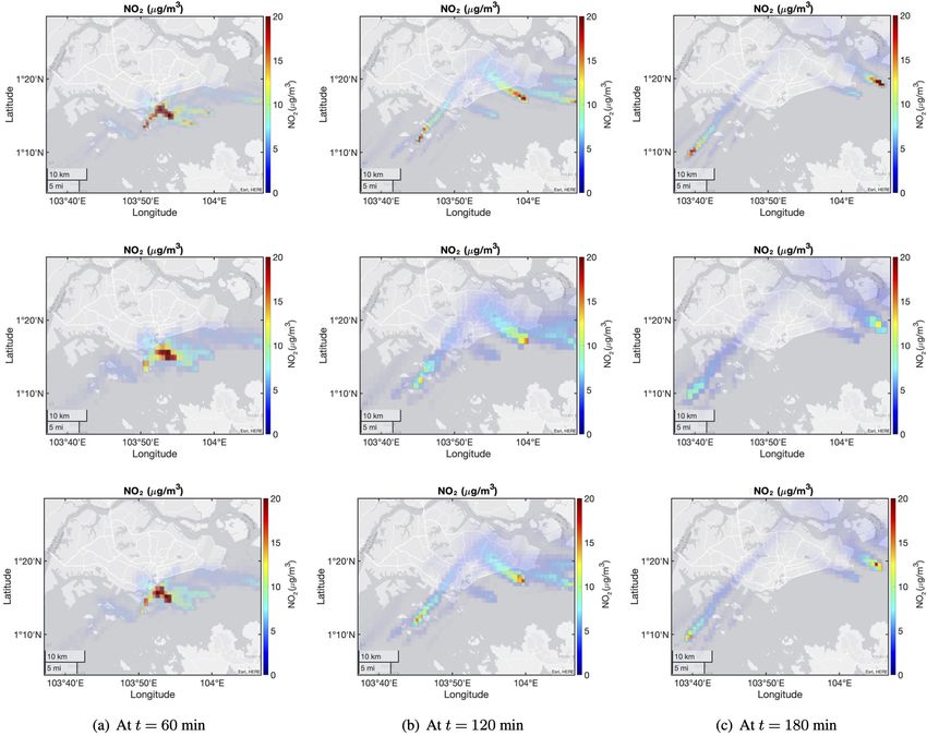
4510                             K. Pan et al.: Development of a moving point source model in EPISODE–CityChem v1.3

based model that assumes the dispersion of air pollutant to       on NOx and ozone (O3 ) in the eastern Atlantic and Western
follow a Gaussian distribution. Merico et al. (2019) applied a    Europe by using an Eulerian model CAMx. Karl et al. (2020)
steady-state Gaussian-based model – ADMS-5 – to estimate          investigated the particle concentrations in the ship plumes
the dispersion of emissions from ships which are mainly in        by coupling an aerosol dynamic model MAFOR (Multicom-
the hoteling and maneuvering phase in the harbor area of          ponent Aerosol FORmation) with a 3D Eulerian chemistry
an Italian port city of Bari. The same model was also used        transport model EPISODE–CityChem. In these studies, the
by Cesari et al. (2016) for a case study of ship emissions in     chemistry transport models (mainly Eulerian models) have
Brindisi, Italy. Another popular steady-state Gaussian plume      shown the ability of predicting the pollutant concentrations
model, AERMOD, recommended by United States Environ-              at the locations of interest and hence are a good approach for
mental Protection Agency (EPA) was also widely used by            investigating the environmental impact of ship emissions in
different groups (Gibson et al., 2013; Cohan et al., 2011).       coastal cities.
Abrutytė et al. (2014) employed AERMOD to simulate the               In pollutant dispersion modeling, it is necessary to include
dispersion of NOx from ships in Klaipėda port. AERMOD            an appropriate assumption or model for treating the emis-
was also used by Fileni et al. (2019) and Cohan et al. (2011)     sion sources. For a typical setup of shipping emission disper-
to evaluate the contribution of ships on PM emissions in har-     sion simulation, the definition for an emission source usually
bor cities. The Gaussian plume model is able to save a lot of     depends on the ship status, namely that the ship is at berth
computational cost; however, it suffers from several limita-      (hoteling) or on cruise (maneuvering and cruising). Usually,
tions, such as assuming a steady-state solution, a spatially      the ship at hoteling phase is treated as a fixed point emission
uniform meteorology and straight line trajectories (Bluett        source (Merico et al., 2019; Poplawski et al., 2011; Deniz and
et al., 2004), which make it not suitable under many con-         Kilic, 2010; Lucialli et al., 2011; Formentin, 2017), which is
ditions for air quality modeling. In addition to the simple       a reasonable assumption as the ship stops at the dock and
Gaussian plume models, some advanced, unsteady Gaussian           generates emissions from its chimney as a single point. For
puff models (such as CALPUFF), which can simulate the ef-         the ships under movement, different models have been ap-
fects of time- and space-varying meteorological conditions        plied to treat the emission sources in different studies. Iodice
on pollutant transport, transformation and removal (Bluett        et al. (2017) assumed the emissions from the moving ships
et al., 2004), are developed as well. CALPUFF has been            were generated at multiple fixed points along the predefined
widely used for simulating the dispersion of ship emissions.      navigation route. Saxe and Larsen (2004) used fixed points
Jahangiri et al. (2018) applied CALPUFF to predict the aver-      to represent the average positions of the ships in both maneu-
age values of the ship emissions on the port area of Brisbane,    vering and hoteling modes. Murena et al. (2018) also treated
Australia, for the whole of 2013. Poplawski et al. (2011) and     the ships in maneuvering and navigation modes as fixed point
Murena et al. (2018) also employed CALPUFF to evaluate            emission sources. In another group of studies, a line emis-
the effects of cruise ships on air quality in the harbors of      sion source model was widely applied to simulate the mov-
Victoria, Canada, and Naples, Italy, respectively. Compared       ing ships in maneuvering or cruising mode (Poplawski et al.,
to the Gaussian plume models, the advanced unsteady Gaus-         2011; Kotrikla et al., 2013; Deniz and Kilic, 2010; Lucialli
sian puff models overcome some limitations; for example,          et al., 2011). In the line source (LS) model setup, the ship
the causality effects can be simulated by CALPUFF.                emission is assumed to be constantly emitted along the en-
   Furthermore, a Lagrangian or Eulerian chemistry trans-         tire ship route, which is assumed to be a straight line. In
port model (CTM) that solves the advection–diffusion equa-        some other cases, ships in hoteling or maneuvering modes
tion and the atmospheric chemistry to predict the transport       were treated as area sources (Kotrikla et al., 2013; Formentin,
and chemical reactions of emission species received increas-      2017; Abrutytė et al., 2014); however, this assumption is not
ing attention (Pillai et al., 2012; Gariazzo et al., 2007; Gad-   commonly used to treat ship emissions.
havi et al., 2015). For a Lagrangian CTM, a moving frame              From the above literature review, it is evident that either
of reference is used to predict the trajectories of the pollu-    a (or multiple) fixed point(s) source model or a line source
tion plume parcels. In comparison, an Eulerian CTM uses a         model is commonly used for ships under movement in the
fixed 3D Cartesian grid as the frame of reference to solve the    air pollution dispersion modeling. However, neither of these
continuity equations. Both CTMs have been applied to simu-        assumptions is realistic as the ship position is changing when
late the dispersion of ship emissions. Krysztofiak-Tong et al.    it is moving. The ship movement is not explicitly included in
(2017) evaluated the air pollution contributed from ships and     current air pollution dispersion modeling and leads to a re-
oil platforms in West Africa by using the Lagrangian model        search gap. In this paper, a moving point source (MPS) model
FLEXPART. Shang et al. (2019) and Chen et al. (2018)              that can update the ship positions at different times based on
applied the Eulerian-based WRF-Chem model to simulate             the ship speed and direction and then simulate the emission
the influence of ship emissions on harbor cities in China.        release from the moving ships in the dispersion modeling
Liu et al. (2017) studied the impact of ship emissions on         was hence developed. The new developed MPS model was
the Shanghai urban area by using the WRF–CMAQ model.              integrated into the 3D Eulerian chemistry transport model
Huszar et al. (2010) evaluated the effects of ship emissions      EPISODE–CityChem (Hamer et al., 2020; Karl et al., 2019)

Geosci. Model Dev., 14, 4509–4534, 2021                                           https://doi.org/10.5194/gmd-14-4509-2021
K. Pan et al.: Development of a moving point source model in EPISODE–CityChem v1.3                                        4511

and applied to predict the dispersion of NO2 species gener-      and vertical eddy diffusivities; and Ri and Si represent the
ated by the ships in cruising mode in a simplified simulation,   source and sink terms. The estimation of eddy diffusivities is
and the simulated results were compared to those obtained        based on the mixing length theory (K-theory) (Slørdal et al.,
by using LS and fixed point source (FPS) models. In addi-        2003). In the simulation, the emission source term, wind
tion, the new MPS model was applied to a real case study         field and other meteorological conditions are assumed to be
to predict the concentrations of NO2 and PM2.5 species con-      hourly constant. The emission species is simulated until it is
tributed by all ships around the city of Singapore, and the      fully diluted or outside of the simulation domain. The photo-
simulated results were compared to the measured values in        chemistry simulated in the Eulerian grid has several options,
different observation stations. The MPS model introduces a       such as EMEP45 (Walker et al., 2003), EmChem03mod and
new approach for treating the ships and other objects un-        EmChem09mod (Simpson et al., 2012), that are modified or
der movement in the atmospheric dispersion modeling and          updated from the European Monitoring and Evaluation Pro-
will increase the knowledge of the atmospheric environment       gramme (EMEP) (Simpson, 1995). In this study, the chemi-
modelers. The model setups and important simulation results      cal scheme applied is EmChem09mod.
are presented in this paper.                                        In the sub-grid receptor model, the pollutants gener-
                                                                 ated by emission sources (either a point or a line source)
                                                                 are calculated by using simple Gaussian models. The LS
2     Methods                                                    model used in the EPISODE–CityChem package is a steady-
                                                                 state integrated Gaussian plume model (HIWAY-2) with
The MPS model developed in this paper was integrated
                                                                 a simplified street canyon model (SSCM), which affects
into the chemistry transport model, EPISODE–CityChem
                                                                 the concentrations on the receptor points close to the line
(Hamer et al., 2020; Karl et al., 2019), which is an open-
                                                                 source (usually within an influence distance of 500 m).
source Fortran-based code. EPISODE–CityChem is a city-
                                                                 The emitted mass from line sources is integrated into the
scale chemistry extension of the dispersion model EPISODE,
                                                                 3D Eulerian model in each simulation time step. For the
which was originally developed by Slørdal et al. (2003) and
                                                                 point source, a Gaussian segmented plume model, SEG-
Slørdal et al. (2008). In this section, the dispersion model,
                                                                 PLU (Walker and Grønskei, 1992), with the use of a Weak-
the MPS model, simulation setups and configurations of the
                                                                 wind Open Road Model (WORM) (Walker, 2011) meteoro-
case studies are introduced.
                                                                 logical pre-processor (WMPP) is implemented to treat the
2.1    Dispersion model                                          pollutants released from an individual point source as dis-
                                                                 crete emissions of finite length plume segments that emit-
EPISODE–CityChem simulates the transport, chemical reac-         ted in each time interval (1t). In the calculations, the plume
tions and deposition of pollutant species in both a 3D Eule-     rise (due to buoyancy or momentum) is estimated based
rian grid and a ground-level sub-grid (Hamer et al., 2020;       on Briggs’s algorithms (Briggs, 1969, 1971, 1975), which
Karl et al., 2019). A typical Eulerian grid has a horizon-       consider the different atmospheric stability conditions (such
tal resolution of 1 km by 1 km, while the vertical grid size     as neutral-unstable and stable conditions). The effects of
varies from several meters (near the ground) to several hun-     stack downwash (Briggs, 1973) and plume penetration (Weil
dreds meters (higher layer), with a total height up to sev-      and Brower, 1984) on plume height are considered as well.
eral kilometers. The sub-grid has a better resolution with a     The transport, growth, chemical reaction and deposition of
typical size of 100 m by 100 m horizontally. The governing       the plumes are estimated based on the local meteorologi-
advection–diffusion and mass conservation equations for the      cal conditions where the plumes stay, and the plume mass
averaged concentrations in the main Eulerian grid model are      is integrated into the Eulerian grids when the segmented
indicated as                                                     plume grows to a predefined size (usually when σy /dy = 4 or
                                                                 σz /dz = 4, where σy and σz are Gaussian dispersion length
∂Ci ∂(uCi ) ∂(vCi ) ∂(wCi )                                      scales in the cross-wind direction and the vertical direction
      +           +         +           =
 ∂t       ∂x          ∂y          ∂z                             for a plume, and dy and dz are the horizontal and vertical
                                                                 sizes of an Eulerian grid cell). The existing plumes contribute

 ∂           ∂Ci       ∂          ∂Ci
      K (H )       +       K (H )                                to the concentrations in the sub-grid receptors. The emission
∂x           ∂x       ∂y          ∂y
                                                               concentration at the receptor points is finally estimated as
    ∂          ∂Ci
+        K (z)       + Ri − Si ,                           (1)   the sum of the Eulerian grid concentration and contributions
   ∂z           ∂z                                               from line and point sources, described as Eq. (3).
∂u ∂v ∂w                                                                         L             P
  +   +    = 0,                                            (2)    t      t−1
                                                                                 X             X
∂x ∂y   ∂z                                                       Crec = Cm   +         Clt +         Cpt ,                  (3)
                                                                                 l=1           p=1
where Ci is the concentration of species i (i = 1 : N, where
N is the total number of species); u, v and w are the three              t is the receptor point concentration at time t, C t−1
                                                                 where Crec                                                m
wind velocity components; K (H ) and K (z) are the horizontal    is the Eulerian grid concentration at the previous time step

https://doi.org/10.5194/gmd-14-4509-2021                                           Geosci. Model Dev., 14, 4509–4534, 2021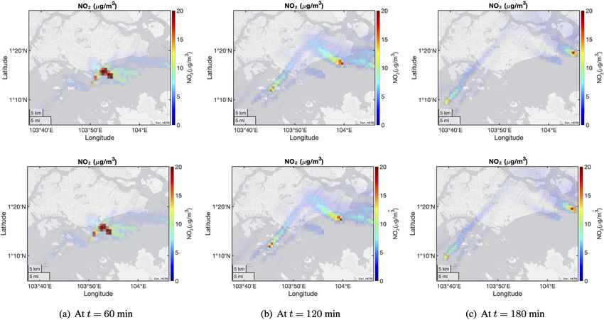
4512                                         K. Pan et al.: Development of a moving point source model in EPISODE–CityChem v1.3

Figure 1. Illustration of the moving point source model. The ship variables in the figures are explained in Table 1.

Table 1. Setup of the moving point source model.

   Parameter                  Description                                                         Value       Note
                                                                                                              (1) us = 0 m s−1 : fixed point (e.g., ships at berth);
   Speed (us )                speed at which point source is moving                          > 0 m s−1
                                                                                                              (2) us > 0 m s−1 : moving point (e.g., ships under
                                                                                                              cruise).
   Direction (9)              direction at which point source is moving                         0–360◦        0◦ : north; 90◦ : east; 180◦ : south; 270◦ : west.
                                                                                                              (1) θ = 0◦ : moving straightly (Fig. 1a);
   Turning angle (θ )         ship turning angle                                          −360–360◦           (2) θ > 0◦ : turning clockwisely (Fig. 1b);
                                                                                                              (3) θ < 0◦ : turning counterclockwisely (Fig. 1b).
                              time that ship starts moving in each simula-                                    (1) 0 s 6 ts1 63600 s if θ > 0◦ (when ship is moving
   Start time (ts1 )                                                                          0–3600 s
                              tion hour                                                                       straightly, as shown in Fig. 1a);
                                                                                                              (2) in current version, ts1 = 0 s if θ 6 = 0◦ (when ship
                                                                                                              is moving in a curve, as shown in Fig. 1b).
                                                                                                              (1) 0 s 6 ts2 6 3600 s if θ > 0◦ ;
                              time that ship stops moving in each simula-
   Stop time (ts2 )                                                                           0–3600 s        (2) in current version, ts2 = 3600 s if θ 6 = 0◦ ;
                              tion hour
                                                                                                              (3) ts1 < ts2 .

 Note that in each simulation hour, all five variables are assumed constant and only need to be updated hourly.

(estimated by Eq. 1), Clt and Cpt are the concentrations con-                                MPS model is hence developed to fill the gap in the pollutant
tributed from line and point emission sources, and L and                                     dispersion modeling.
P are the total numbers of line and point emission sources.                                     In the MPS model, five new parameters are defined to
In the sub-grid modeling, the stack downwash, dry and wet                                    determine the ship movement route, as presented in Fig. 1.
deposition, and plume rise and penetration are considered                                    The most important parameters are ship speed and direc-
as well, and the photochemistry applied is the EP10-Plume                                    tion, which can be easily captured from the maritime online
scheme (Karl et al., 2019). More details about the EPISODE–                                  databases, such as MarineTraffic. Three additional parame-
CityChem software can be found in the papers written by                                      ters, namely turning angle, start and stop time, are defined
Hamer et al. (2020) and Karl et al. (2019).                                                  to provide the options to customize the ship movement when
                                                                                             more accurate ship travel information is obtained. The new
                                                                                             variables for each ship are only updated hourly and hence
2.2    The moving point source model                                                         kept constant for each simulation hour. The detailed descrip-
                                                                                             tions about the five model parameters are summarized in Ta-
As found from the literature review, LS and FPS models                                       ble 1.
are the common approaches to simulate the emissions gen-                                        Based on these five variables, the ship position is estimated
erated by the moving ships; however, they are not realistic                                  and updated in each simulation time step (1t). As shown in
as they cannot update the instantaneous ship positions. The                                  Fig. 2, ship emission is assumed to be emitted in a virtual

Geosci. Model Dev., 14, 4509–4534, 2021                                                                            https://doi.org/10.5194/gmd-14-4509-2021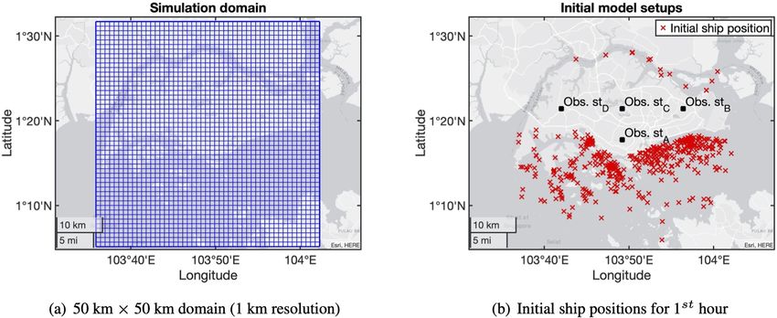
K. Pan et al.: Development of a moving point source model in EPISODE–CityChem v1.3                                                    4513

point of the short ship line that represents an average ship
position for each individual time step. The emitted plume is
then treated by using the SEGPLU model in EPISODE. As
mentioned above, the parameters (such as plume size and lo-
cation) of each individual plume were updated in each time
step, and then their contributions to the 3D Eulerian cell and
sub-grid receptors were calculated. In this model, the ship
movement parameters, mainly ship speed, direction and turn-
ing angle, are constant for each simulation hour, and hence
the virtual point is usually taken as the middle point of the           Figure 2. Virtual point for plume release in each time step (1t).
short travel distance during each 1t. Apparently, the ship
and plume positions are more realistic when the time step
is smaller. For the time step in which the ship starts or stops         2.3.1   Simplified study
moving, the estimation of the virtual point takes the time fac-
tor into account, as presented in Eqs. (4) and (5).                     As shown in Fig. 3, the simulation is first conducted to in-
                       ti − ts1                                         clude only a group of moving ships. The simulation domain
x i = x i−1 + 0.5dx i           ; (if ti−1 ≤ ts1 ≤ ti ),          (4)   is set for a 70 km by 70 km area, with a horizontal resolution
                          1t
                             ts2 − ti−1                                 of 1 km by 1 km in the reference case as suggested by Hamer
x i = x i−1 + dx i − 0.5dx i             ; (if ti−1 ≤ ts2 ≤ ti ), (5)   et al. (2020) and Karl et al. (2019), and the domain has 13
                                 1t
where x i is the virtual position (x, y) of a ship during the           vertical layers, with a height of 10 m in the ground layer and
ith time step in each simulation hour, dx i = us (ti − ts1 ) (or        500 m in the top layer (total height is 3500 m). The sub-grid
us (ts2 −ti−1 )) is the actual ship travel distance in the ith time     receptor points (100 m by 100 m horizontal resolution) are
step, ti = i1t is the actual time difference from the start of          created with a receptor height of 1.5 m above ground. In ad-
each simulation hour for the ith time interval and us is the            dition, a data point is selected around the coastline, as shown
ship velocity. As mentioned above, the five parameters in the           in Fig. 3, to record the concentrations of emission species at
simulation are only updated each hour, assuming that the ship           every simulation time step.
is moving in a straight line or a curve with a constant speed              To simplify the simulation, a constant meteorological con-
during each hour. This is actually a limitation for the current         dition taken from two weather stations (as shown in Fig. 3b),
version of the MPS model compared to a real ship if its move-           one in the south of Singapore and another in the north of
ment parameters change frequently; however, the model used              Singapore, was applied to the entire simulation period. The
in this study is to address the idea of a MPS model that has            details of the weather conditions are shown in Table 2, where
the potential of tracking the ship movement and then better             the wind inputs in two weather stations were assumed to
simulates the dispersion details of ship emissions. The cur-            be 2 m s−1 and 180◦ (blown from south to north). A built-
rent version of MPS model provides an alternative option for            in meteorological pre-processor, MCWIND, was used to
simulating the dispersion of ship emissions in a harbor city.           first guess and estimate the local wind speed and direc-
In addition, it should be highlighted that it is possible to de-        tion in the simulation domain, based on the input values
fine an arbitrary ship movement by using the MPS model,                 from the weather stations, and then they were adjusted to
once the real ship movement data collected at different time            the given topography to obtain the 3D divergence-free and
are added to the MPS input files in the simulation. In this             mass-consistent diagnostic wind field (Hamer et al., 2020).
study, the turning angle (θ ) is set as 0◦ for all moving ships,        Other meteorological parameters (such as vertical temper-
and the start time (ts1 ) and stop time (ts2 ) for all moving ships     ature gradient) in the simulation area were also estimated
are assumed to be 0 and 3600 s respectively, due to the lack            by MCWIND. In this paper, the calculated wind field in the
of such information for each ship.                                      ground-level layer for the dispersion modeling is shown in
                                                                        Fig. 4.
2.3   Simulation setup                                                     In the simplified simulation, a total number of 44 ships
                                                                        with different types and sizes are included. The ships are
The purpose of this study is to evaluate the new developed              separated into two groups, where one group (22 ships) is
MPS model, and two simulations are conducted in the Sin-                assumed to move towards China and another is heading to
gapore area in this paper. One is a simplified dispersion sim-          Europe. The ship data, such as ship position, speed, direction
ulation that only includes moving ships with simplified input           and gross tonnage, are collected from online ship resources
conditions, and the results by using the MPS model are com-             (such as VesselFinder). In order to better illustrate the fea-
pared with the LS and FPS models. Another is a real case                ture of the new MPS model and also compare its results with
study that simulates all the ships around the city of Singapore         those simulated by the LS and FPS models, only ships on the
using the new model and compares them with the concentra-               China–Europe route (west–east direction) are kept as the ini-
tions of emission species measured in different stations.               tial conditions by removing all other ships (such as those are

https://doi.org/10.5194/gmd-14-4509-2021                                                   Geosci. Model Dev., 14, 4509–4534, 2021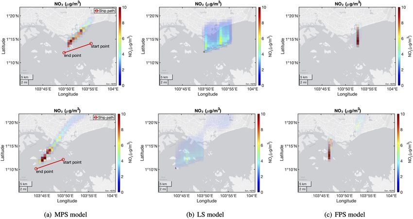
4514                                 K. Pan et al.: Development of a moving point source model in EPISODE–CityChem v1.3

Figure 3. Configuration of the simulation domain in Singapore used in the simplified simulation. Ships to China are indicated by blue circles,
and ships to Europe are indicated by red crosses; lines denote ship routes.

Table 2. Meteorological inputs applied in MCWIND pre-processing utility for the simplified simulation.

                             Ust1 (m s−1 )       WDst1 (◦ )        Tst1 (◦ C)      RHst1 (%)         Ust2 (m s−1 )       WDst2 (◦ )
                             2.0                 180               32              64.3              2.0                 180
                           U : wind speed; WD: wind direction; T : temperature; RH: relative humidity; st1 and st2: weather station 1 and
                           2.

                                                                                     sion factor equation (Eq. 6) proposed in the MEET method,
                                                                                     based on a ship’s specifications such as ship type, speed and
                                                                                     gross tonnage, as shown in Fig. 5. During the simplified sim-
                                                                                     ulation, the emission rates for each ship were constant as
                                                                                     the ship operating conditions were unchanged, and no back-
                                                                                     ground concentrations were used. In addition, the chimney
                                                                                     height is assumed to be 30 m for the large size ships (such as
                                                                                     the liquid bulk ships) and 10 m for the small ones (such as
                                                                                     the leisure ships), while exit gas is assumed to be at 20 m s−1
                                                                                     with 300 ◦ C for all ships. The ship building height for each
                                                                                     ship is set as 5 m below than the chimney height, and the
                                                                                     width is assumed to be 20 m for the large-size ships and 5 m
                                                                                     for the small ones. These choices have a very minor effect
                                                                                     on the results (Appendix C). In this study, the ship emission
Figure 4. The 2D plot of ground-level diagnostic wind field calcu-
lated by MCWIND for the simplified dispersion modeling.
                                                                                     sources were treated by using three different models, namely
                                                                                     moving point, fixed point and line sources, and the simu-
                                                                                     lated emission profiles were compared. The simulation se-
                                                                                     tups are summarized in Table 3. In addition, sensitivity stud-
at berthed or moving in a north–south direction), as shown in                        ies were conducted by changing the mesh density, simulation
Fig. 3, and no new ships are included in the simulation. The                         time step and emission source setups (such as exit veloc-
dispersion modeling was conducted until all ships moved out                          ity, chimney height and ship building dimensions), and the
of the simulation domain. During the entire simulation, all                          simulated concentration profiles for different species (such
ships were assumed to move straightly (θ = 0◦ ), and the ship                        as NO2 , SO2 and PM2.5 ) were compared as well. The simu-
parameters (such as speed and direction) were assumed to be                          lation results for the sensitivity studies are presented in Ap-
unchanged.                                                                           pendices A–D.
   The ships are then divided into different categories (such                                         "                                  #
as liquid bulk ships, dry bulk carriers, containers and cargo)                                     X       X
based on those defined in the MEET (Methodologies for esti-                          Etrip,i,j,k =      tm     Pe × LFe × EFe,i,j,k,m ,           (6)
                                                                                                        m          e
mating air pollutant emissions from transport) methodology
by Trozzi and Vaccaro (1999) and Trozzi (2010). The emis-                            where Etrip is the emission over a trip (kg), EF is the emission
sion rates of main species (such as NOx and PM) for each                             factor (kg kWh−1 ), LF is the engine load factor (%), P is the
ship were then estimated by using the power-based emis-                              engine power (kW), t is time (hours), e is the engine category

Geosci. Model Dev., 14, 4509–4534, 2021                                                                     https://doi.org/10.5194/gmd-14-4509-2021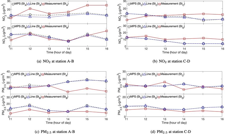
K. Pan et al.: Development of a moving point source model in EPISODE–CityChem v1.3                                               4515

Table 3. Setups of shipping emission dispersion modeling.

  Case     Emission source   Time step      Horizontal resolution             Vertical resolution
  1        MPS model         1t = 15.8 s    dx = dy = 1 km (nx = ny = 70)     varying dz (dz1−2 = 10 m. . . dz13 = 500 m) with total
                                                                              height of 3.5 km
  2        LS model          1t = 15.8 s    dx = dy = 1 km (nx = ny = 70)     varying dz (dz1−2 = 10 m. . . dz13 = 500 m) with total
                                                                              height of 3.5 km
  3        FPS model         1t = 15.8 s    dx = dy = 1 km (nx = ny = 70)     varying dz (dz1−2 = 10 m. . . dz13 = 500 m) with total
                                                                              height of 3.5 km
  4        MPS model         1t = 10 s      dx = dy = 1 km (nx = ny = 50)     varying dz (dz1−10 = 10 m and dz11−30 = 20 m) with
                                                                              total height of 0.5 km

                                                                    Singapore are included in the simulation, the ships are only
                                                                    updated each hour and their rates are estimated by using
                                                                    MEET method (Eq. 6) based on the ship information ob-
                                                                    tained from the online resource VesselFinder. Then the mete-
                                                                    orological conditions obtained from Meteorological Service
                                                                    Singapore in each hour are applied to the simulation, while
                                                                    the concentrations of emission species obtained from the Na-
                                                                    tional Environment Agency in Singapore were selected as the
                                                                    background concentrations. In this study, all other model se-
                                                                    tups and configurations are listed as case 4 in Table 3.

                                                                    3     Results and discussion

                                                                    In this section, the results for two studies are presented. The
                                                                    first one (Sect. 3.1 and 3.2) results from comparing the MPS
Figure 5. Shipping emission dispersion modeling with MEET           model with LS and FPS models for a simplified simulation.
method (Trozzi, 2010).                                              The air pollution dispersion modeling was first conducted
                                                                    with only one ship in the simulation domain, and the plume
                                                                    structures simulated by different emission models are com-
(main or auxiliary engine), i is the pollutant species (such as     pared. The emission source models were then applied to the
NOx , PM), j is the engine type (slow-, medium- and high-           additional simulation cases (cases 1–3) that include more
speed diesel engine, gas turbine, and steam turbine), k is the      ships in the China–Europe direction near Singapore. The in-
fuel type (bunker fuel oil, marine diesel/gas oil, gasoline), m     stantaneous results and the hourly averaged NO2 values sim-
is the ship operation mode (cruising, hoteling, maneuvering).       ulated by different emission models are presented, as both
                                                                    of them are important for evaluating the impact of the pollu-
2.3.2    Real case study                                            tant emissions on the locations of interest. The second part
                                                                    (Sect. 3.3) is a real case study (case 4) that compares the
The MPS model was applied to a real case study in this pa-          predicted hourly averaged NO2 and PM2.5 concentrations by
per as well. The hourly averaged emission values for several        the MPS model at the observation stations with the measured
hours (11:00 to 16:00 on 23 April 2020) in Singapore were           data.
simulated by using the MPS model, and the results at differ-
ent observation stations were compared to the measured data.        3.1     Simplified simulation – preliminary comparisons of
The model setups (such as the grid size) and numerical meth-                different emission source models
ods (such as MEET method for emission rate calculation) are
the same as those used in the simplified simulation, except         The new MPS model was first tested by simulating only one
for those (such as the meteorology and background concen-           ship, which moves from the east side to the west side. In
trations) introduced in this section. The configurations and        this preliminary simulation, the ship movement parameters
setups of the simulation are shown in Fig. 6.                       are constant, and all other conditions such as wind speed and
   The first difference in this real case study compared to the     direction are the same as mentioned in Table 2.
simplified simulation is that all the ships around the city of

https://doi.org/10.5194/gmd-14-4509-2021                                                Geosci. Model Dev., 14, 4509–4534, 2021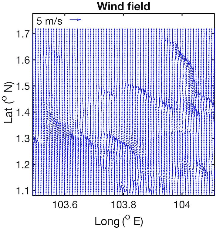
4516 K. Pan et al.: Development of a moving point source model in EPISODE–CityChem v1.3
Figure 6. Configuration of the simulation domain used in the real case simulation.
Figure 7a presents the instantaneous NO2 concentration from the ship point and then diluted. Since the ship position
near the ground simulated by the MPS model. Based on the is assumed to be unchanged during each hour in the simula-
2D plots, it clearly shows that the species concentration in- tion, the emission is distributed in a much smaller area with
side the plume is gradually reduced in the opposed direc- a much larger concentration compared to the other two mod-
tion to the ship movement, which is reasonable. As the ship els. Clearly, the FPS model cannot reveal the effects of ship
moves in the west–south direction and keeps emitting emis- movement on emission dispersion.
sions at different positions along its route, the early gen-
erated emission are transported by wind further north and 3.2 Simplified simulation – results for case studies with
then diluted, and hence the emission plume is formed with more ships
minimum concentration on the east side and peak value on
the west side. The simulated results indicate that the MPS After comparing the three emission source models for only
model gives a quite reasonable prediction for the distribution one ship simulation, the three models were applied to a sim-
of emissions released by a moving ship. plified study (cases 1–3) with 44 ships involved, in order to
In comparison, the LS model gives quite different results, further evaluate the performance of different models for pre-
as shown in Fig. 7b, with the simulated NO2 species dis- dicting the effects of moving ships on air quality in coastal
tributed in a much wider area with a relatively smaller peak cities. Both of the instantaneous and average results are pre-
concentration. In the dispersion modeling, a line source is a sented in this section to fully compare the different emission
very common model for treating a moving ship, assuming models. The meteorological conditions and simulation setups
that the ship continuously generates emissions along the en- are the same as presented in Tables 2 and 3.
tire line in the simulation. As a result, more emissions appear
near the entire ship route and are then gradually diluted in the 3.2.1 Simulated results by using the moving point
downwind side. Compared to the real condition, it is unrealis- source model
tic as the ship keeps moving and is not able to emit emissions
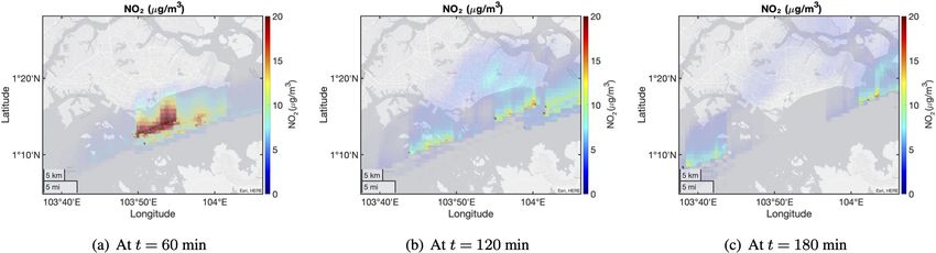
from the entire ship route simultaneously. Furthermore, since In the case study for more moving ships, the simulation was
the total emission rates (g s−1 ) generated by the ship are the first conducted by using the MPS model (case 1), and the
same for the MPS and LS models, the NO2 emission rate at instantaneous ground-level NO2 concentrations at different
each point along the ship route (or emission rate intensity, time around the Singapore area are plotted in Fig. 8. Based
g s−1 m−1 ) in the LS model is much smaller than the MPS on the 2D plots, it can be seen that the NO2 emission moves
model. Hence, the maximum NO2 concentration generated north from the ship positions and forms the higher concentra-
by the LS model has a relatively smaller value than the MPS tion at t = 60 min compared to other simulation time, as most
model. of ships are passing the same area during the first 60 min
In addition, the simulated emission profiles by using a FPS (Fig. 3c). The gas species then moves to the west and east
model are illustrated in Fig. 7c. The FPS model is another directions as the two groups of ships move towards their des-
commonly used assumption for treating the moving ship in tinations, and the gas concentration is continuously diluted
the literature. In this study, the moving ship is assumed to in the following simulations as the ships keep moving out of
stay in the middle point of the ship routine in each hour. As the Singapore area.
shown in Fig. 7c, the NO2 emission is blown north by wind Figure 9 illustrates three vertical NO2 concentration pro-
files (west–east vertical plane) at t = 60 min. From these fig-
Geosci. Model Dev., 14, 4509–4534, 2021 https://doi.org/10.5194/gmd-14-4509-2021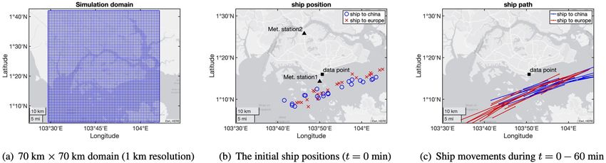
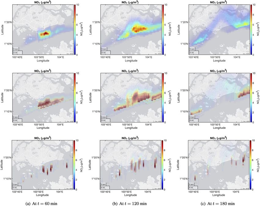
K. Pan et al.: Development of a moving point source model in EPISODE–CityChem v1.3                                             4517

Figure 7. Instantaneous NO2 concentrations near the ground generated by one moving ship. Top row: at t = 60 min; bottom row: at t =
120 min.

Figure 8. Instantaneous NO2 concentrations near the ground by using the MPS model (case 1).

ures, it can be seen that less NO2 species arrives on the            in the downwind direction, the plumes are diluted vertically
ground when the plumes are closer to ships (Fig. 9a), and            until they fully disappear, as shown in Fig. 9c.
then the gas species are transported vertically to the ground            In addition, the time history of NO2 concentration
as the plumes move in the downwind direction (Fig. 9b).              recorded at the data point (shown in Fig. 3b) is also plot-
This is mainly attributed to the plume rise effects when the         ted as shown in Fig. 10, where it indicates that there are two
gas species exits the ship chimney with a certain velocity (in       peaks for NO2 concentration when using the MPS model.
the simplified simulation, the exit velocity is assumed to be        The time history is reasonable. Based on the NO2 curves,
20 m s−1 for all 44 ships), and then the gas species are blown       it indicates that the emission species generated by the ships
by the wind (south to north) and only reach the ground at a          take around 30 min to reach the data point, and hence the two
certain distance in the downwind direction. As a result, the         peaks should be induced by the transport and accumulation
peak NO2 concentrations at ground level appear on the lo-            of emissions generated during the first 60 min. As shown in
cations that are far away from the ship routes but not near          Fig. 11, a large group of ships pass by or are close to the data
the ships, as shown in Fig. 8. As the emissions move further         point during the first 30 min and lead to a continuous emis-

https://doi.org/10.5194/gmd-14-4509-2021                                                Geosci. Model Dev., 14, 4509–4534, 2021
4518                               K. Pan et al.: Development of a moving point source model in EPISODE–CityChem v1.3

Figure 9. Vertical NO2 profiles (west–east direction) at t = 60 min.

                                                                       trated in a small region (as shown in Fig. 3), the integration
                                                                       of simulated NO2 emission generated by line sources induces
                                                                       a higher peak concentration than the MPS model (Fig. 13a),
                                                                       although the emission rate intensity for each line source is
                                                                       smaller as mentioned in Sect. 3.1. As expected, when the
                                                                       ships are separated, the maximum NO2 concentration for the
                                                                       line source becomes smaller than the MPS model, as shown
                                                                       in Fig. 13b and c.
                                                                          The NO2 time history curve for the LS simulation is also
                                                                       obtained as shown in Fig. 10. Compared to the MPS model,
Figure 10. Time history of NO2 concentration at the data point sim-    this simulated NO2 concentration reaches its peak at around
ulated by using different emission source setups.                      t = 65 min and then is kept for around 15 min before it drops.
                                                                       In EPISODE–CityChem, hourly based simulations are con-
                                                                       ducted, and all the conditions such as meteorological param-
sion accumulation to form the first peak concentration, and            eters and emission setups are constant for every 60 min sim-
another group of ships pass by the data point later (from 40           ulation. As shown in Figs. 3 and 12, more ships pass the data
to 60 min) to generate the second peak value. After 60 min,            point during the first 60 min and less ships pass by during
most of the ships have passed the data point (Fig. 12), and            the second simulation period (t = 60–120 min). When the
hence the NO2 concentration is continuously decreased. The             LS model is used, a constant total NO2 emission rate is gen-
time series of 2D plots in Fig. 8 and the NO2 concentration            erated during the first simulation period (t = 0–60 min) and
curve in Fig. 10 reveal that the effects of ship movements             continuously affects the data point, leading to a concentration
on emission distributions can be well captured by using the            rise in the NO2 curve to the peak value at around t = 65 min
MPS model.                                                             (Fig. 10). Then the emission generation and dilution reach
                                                                       an equilibrium condition to maintain a constant peak con-
3.2.2   Comparison of three emission source models –                   centration for a while, until the emissions generated by the
        instantaneous value                                            ships in the second simulation period arrive at the data point.
                                                                       A smaller total emission rate is generated by the smaller
In the simplified case study, the simulation was then con-             amount of ships (during t = 60–120 min) near the data point
ducted by treating each moving ship as a line source (case             area, and hence the local concentration at the data point is re-
2). The instantaneous NO2 concentrations contributed from              duced, shown as the NO2 curve in Fig. 10. Clearly, the NO2
the two groups of ships are plotted in Fig. 13 for different           concentration history obtained by the LS model cannot reveal
simulation times. Compared to the MPS results (Fig. 8), it             the effects of real ship movements on emission dispersion,
clearly shows a much wider NO2 distribution in the Singa-              and hence it is not an appropriate assumption for simulating
pore area when using the LS model to simulate the moving               the instantaneous emission dispersion for ships in cruising
ships, due to the continuous emission generation along the             mode compared to the MPS model.
entire ship routes. For the LS model, the generated emis-                 In addition, the simulation was conducted by using the
sions have the continuous impact on a specific area, while             FPS model as well, assuming that the ships are staying at the
the emissions emitted by the MPS model only have transient             middle points of the ship routes in each hour. The ground-
impact on the same area. As a result, when ships are concen-

Geosci. Model Dev., 14, 4509–4534, 2021                                                https://doi.org/10.5194/gmd-14-4509-2021
K. Pan et al.: Development of a moving point source model in EPISODE–CityChem v1.3 4519
Figure 11. Ship movements during t = 0 − 60 min.
Figure 12. The ship initial positions and movements during t = 60–120 min.
level NO2 distribution profiles are presented as Fig. 14. As source models are compared as well, and the average NO2
expected, the emissions are distributed as separated plume concentrations near the ground at different simulation time
segments, which are clearly not accurate. In Fig. 10, the NO2 are presented in Fig. 15. Based on the 2D plots in Fig. 15,
history curve for the fixed point assumption has the smallest it can be seen that the average NO2 profiles using the FPS
peak value, as less NO2 emission can be blown to the loca- model are much different from the other two setups. As dis-
tion of the data point. The individual plume segments and the cussed above, the FPS setup is clearly inappropriate for mod-
smallest single-peak NO2 time history indicate that the FPS eling the moving ships.
model is an inaccurate approach for simulating the emission The hourly averaged 2D plots in Fig. 15 also indicate that
release and dispersion from the moving ships. Based on the the simulated NO2 emissions by using the MPS and LS mod-
comparisons of the simulation results by using three differ- els are distributed in a similar area. This is because the emis-
ent emission models, this suggests that the new developed sions for each ship are emitted along the same ship route for
MPS model can simulate more realistic ship movement and two models, although the location of NO2 species generated
then instantaneous emission concentrations generated by the by a MPS model changes along the ship route, while the LS
moving ships. model emits emissions along the entire route continuously.
As a result, the accumulated NO2 emissions cover a similar
3.2.3 Comparison of three emission source models – area for the two model setups and then generate similar re-
average value sults in the hourly averaged evaluations. However, the details
of the NO2 distributions (such as the peak concentration lo-
The simulation results in previous sections are the instanta- cations and values) are different for the two emission models,
neous NO2 concentrations. In emission dispersion modeling, due to their natures of treating the emission generation dif-
the average results (usually hourly based) are also impor- ferently in the dispersion modeling. As shown in Fig. 15, the
tant as they can be used for policy decision and for eval- LS model may overestimate the average NO2 concentrations
uating the long-term environmental impact. In this section, in some locations, compared to the MPS model.
the hourly averaged results by using three different emission
https://doi.org/10.5194/gmd-14-4509-2021 Geosci. Model Dev., 14, 4509–4534, 20214520 K. Pan et al.: Development of a moving point source model in EPISODE–CityChem v1.3
Figure 13. Instantaneous NO2 concentrations near the ground by using the LS model (case 2).
Figure 14. Instantaneous NO2 concentrations near the ground by using the FPS model (case 3).
The hourly averaged NO2 concentrations at the data point the emission values at the four stations compared to the mea-
for three emission source models are presented in Fig. 16. sured results, although there are still gaps between simula-
The concentration curves again indicate that the MPS and tion and measurement. The differences may be attributed to
LS models predict comparable average NO2 concentrations, the following aspects. First of all, only the emissions gener-
while the FPS model gives a much different result. The sim- ated from ships around Singapore were included in the sim-
ulation results suggest that the MPS model should be able to ulation; however, in the real world, the emissions measured
provide an alternative option to predict the hourly averaged in the observation stations should be the results contributed
emission concentrations and distributions in the air pollution from ships and other sources, such as cars and powerplants.
dispersion modeling. In addition, some assumptions were made in the simulation
to simplify the model inputs that could induce different re-
3.3 Real case study – comparison with measurement sults from the real conditions. In the simulation, the me-
teorological conditions (such as wind speed and direction)
are assumed to be hourly constant, although a space-varying
After comparing with the LS and FPS models in a simplified
wind field is estimated based on the input values at multi-
study, the new developed MPS model was applied to the real
ple weather stations, while the real wind and temperature
case by predicting the emission results generated by all ships
are time- and space-varying, which could highly affect the
(including those under cruise and at berth) around the Sin-
dispersion of the emissions generated from ships. A con-
gapore area during a couple of hours. The predicted hourly
stant background concentration was applied for the simula-
averaged NO2 and PM2.5 concentrations are compared to the
tion while the actual value changes in different locations at
observed results obtained from the Singapore National Envi-
different time. For the MPS model, each ship is assumed to
ronment Agency online data resource.
move at constant speed and direction in each simulation hour,
Figure 17 compares the concentrations of NO2 and PM2.5
and no new ships are included until the next hour; however,
predicted by using the MPS model with the values ob-
in the real world, ships’ speed and direction vary frequently,
tained from different observation stations, whose locations
and ships can travel to the selected region at any time. The
are shown in Fig. 6b. Based on the figures, it can be seen
emission inventory or emission rate calculated by using the
that the new developed MPS model can reasonably predict
Geosci. Model Dev., 14, 4509–4534, 2021 https://doi.org/10.5194/gmd-14-4509-2021K. Pan et al.: Development of a moving point source model in EPISODE–CityChem v1.3 4521
Figure 15. Hourly averaged NO2 concentrations near the ground by using different emission models. Top row: MPS model (case 1); middle
row: LS model (case 2); bottom row: FPS model (case 3).
MEET method is based on the empirical equations fitted by
the emission data obtained from a ship database, which in-
cludes ships with different types and sizes operating under
different conditions (such as cruising and hoteling), and the
estimated emission rates may be quite different from the ac-
tual values. Finally, the computational methods and model
setups used in the simulation may not reveal the real process.
The simulation is applied to a city-scale region with rela-
tively coarse mesh setup, and the emission details at specific
locations may not be well captured. The local emission distri-
bution may vary highly due to the effects of different factors,
Figure 16. Hourly averaged NO2 concentrations at a fixed point such as building effect and different surface roughness. The
(“data point” in Fig. 3b) simulated by using different emission chemical reactions of emission species are very complicated
source setups. and may not be well predicted by the chemical mechanism
applied in the simulation, while the physical changes in the
aerosol particles are not simulated by the model.
https://doi.org/10.5194/gmd-14-4509-2021 Geosci. Model Dev., 14, 4509–4534, 20214522 K. Pan et al.: Development of a moving point source model in EPISODE–CityChem v1.3
Figure 17. Comparison of hourly averaged emission concentrations between simulation and measurement at different locations.
The simulation results by using the LS model are also ner in the location of interest; however, the new MPS model
presented in Fig. 17. Compared to the measured data, the could capture the impact of changes in the ship’s course on
NO2 and PM2.5 concentrations predicted by the MPS and LS the emission dispersion and hence provide more options to
models are generally similar, while the MPS model shows the modeler.
slightly better NO2 results at the observation station A, which
is closer to the ships than other stations. Fig. 18 also presents
the overall averaged emission concentrations during the en- 4 Conclusions
tire simulation period predicted by the MPS and LS models,
and it clearly shows that the emission concentrations pre- In this paper, a MPS model was developed to simulate the
dicted by the two models are quite different, especially at emission generation and transport from the moving ships in
the locations close to the ships. The different results for the pollutant dispersion simulations. For the dispersion model-
two models are mainly attributed to the different treatments ing, the common assumption is to use a LS or a FPS model
for the moving ships. However, as the emissions are trans- to treat the emissions generated by the moving ships. Both
ported to the locations far away from the ships (such as at the models cannot update the ship movements within a certain
stations A–D), the differences of the emission concentrations time period (usually an hour), which results in an unrealistic
predicted by the two models become smaller, due to the emis- emission distribution. In the MPS model, the ship movement
sion deposition and dilution. Although it may be expected parameters, including speed and direction, are used to update
that with a large number of ships and for large distances from the ship positions and then to estimate the emission disper-
the sources the LS model and the new MPS model will give sion at different simulation times. The new developed model
similar results, the MPS model is a more realistic represen- was integrated into the city-scale chemistry transport model,
tation of the source and allows for greater granulation of the EPISODE–CityChem, and then was evaluated by simulating
emissions, allows for a swift response of the pollution disper- the atmospheric dispersion of emission species emitted by
sion model to any changes in the ship movement and is ex- the ships in the Singapore area.
pected to be equally accurate across all scales. Based on the The computational results by using the MPS model were
results in this section and the simplified study, it is found that first compared to those obtained from a LS model and a FPS
differences between the LS and the MPS models are small model in simplified simulations. Under the simplified con-
when a large number of ships are moving in a constant man- ditions with a limited number of ships, the results indicated
that the new developed MPS model can simulate the ship
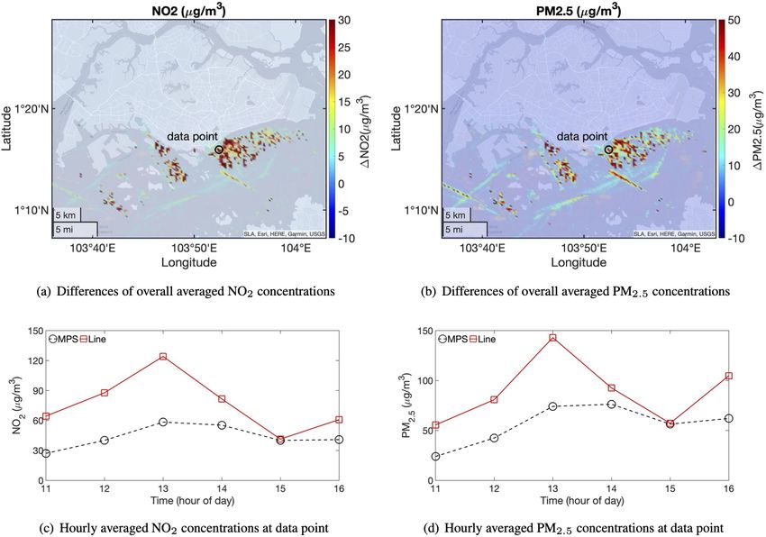
Geosci. Model Dev., 14, 4509–4534, 2021 https://doi.org/10.5194/gmd-14-4509-2021K. Pan et al.: Development of a moving point source model in EPISODE–CityChem v1.3 4523 Figure 18. Emission concentrations during the entire simulation period predicted by the MPS and LS models. Note that in panels (a) and (b), the 2D plots show the differences of the overall averaged concentrations during the entire simulation period (6 h) predicted by using the LS and MPS models (differences = LS results − MPS results). In panels (c) and (d), the curves present the hourly averaged concentrations predicted by two models at the location of the data point shown in panels (a) and (b), where large differences exist. movement and hence predicts more realistic instantaneous In addition, a real case study was conducted as well to fur- concentration profiles for the emission species (such as NO2 ) ther evaluate the MPS model by simulating all ships around generated by the moving ships. In comparison, the LS model the Singapore area. Compared to the measured data, the MPS assumes a continuous and constant emission rate along the model was found to reasonably predict the emission con- entire ship route and then results in much different emis- centrations at different observation stations located in Singa- sion profiles and cannot reveal the instantaneous impact of pore, although gaps still exist due to the different setups and ship movements on air quality in the coastal area. For the configurations between simulations and measurements. The FPS model, separated plume segments were observed in the LS model was compared in the study as well. The predicted simulation. Clearly, it is unrealistic as the emission is con- emission concentrations by the MPS and LS models are quite tinuously generated by the moving ships from different posi- different at the locations close to the ships, while these dif- tions at different time, and a continuous emission distribution ferences become smaller at the locations far away from the should be formed. The hourly averaged values were com- ships as the emission is diluted and deposited. Compared to pared as well for all three models. The comparison shows the measured data, the MPS and LS models perform simi- that the averaged concentration profiles are similar but with larly, while a slightly better NO2 result was found for the local differences for the MPS and LS models, mainly caused MPS model at observation station A, which is closer to the by the different treatments for emission release by the two ships. The real case study together with the simplified study models although the positions of emission release cover the suggests that the MPS model is a more realistic representa- same ship routes. The FPS model again was proven to be an tion of the emission source, and it allows for greater granu- inappropriate assumption for treating the moving emission lation of the emissions and a swift response of the pollution source. dispersion model to any changes in the ship movement, com- https://doi.org/10.5194/gmd-14-4509-2021 Geosci. Model Dev., 14, 4509–4534, 2021
4524                            K. Pan et al.: Development of a moving point source model in EPISODE–CityChem v1.3

pared to the LS and FPS models. The MPS also has a great
potential for a real-time simulation of the shipping emission
dispersion, when used together with the automatic identifi-
cation system (AIS) ship position data. Therefore, the MPS
model should be a valuable alternative for the environmental
society to evaluate the pollutant dispersion contributed from
the moving ships.

Geosci. Model Dev., 14, 4509–4534, 2021                                    https://doi.org/10.5194/gmd-14-4509-2021
K. Pan et al.: Development of a moving point source model in EPISODE–CityChem v1.3                        4525

Appendix A: Parameter study – time step

To further evaluate the MPS model, the time step is investi-
gated. In the reference case (case 1), the calculated time step
is 15.8 s, and in this parameter study, the time step is adjusted
to two different values of 10 s (case S1) and 30 s (case S2) as
shown in Table A1. All other conditions and model setups
for all three cases are the same.
   The instantaneous NO2 profiles at ground level for two
additional time step simulations are plotted in Fig. A1. Com-
pared to the reference case (Fig. 8), it indicates that the NO2
profiles at different simulation time are almost same for all
three cases, although the local emission distributions and
concentrations are slightly different.
   In EPISODE–CityChem, parallel simulations of emis-
sion dispersion are conducted, with one Eulerian main
grid (where dz = dy = 1 km) built up to model the time-
dependent advection and diffusion of emission species in
the 3D space. At the same time, the emissions emitted from
each point source in the sub-grid modeling are treated as fi-
nite Gaussian plume segments generated in each time step.
The plume size and movement (speed and direction) are esti-
mated based on the local meteorological conditions (mainly
temperature, wind speed and direction) of the Eulerian grid
cell, where the plume stays. In next time step, the plume po-
sition is updated, and then its size and movement parameters
are re-calculated based on the new meteorological conditions
of the main grid cell, where the plume segment is transported.
In addition, when the length scale of the segmented plume
(σy or σz , which is highly affected by the meteorological con-
ditions such as wind speed and temperature) reaches a pre-
defined value (usually one-fourth of the Eulerian grid size),
the plume mass is integrated into the main Eulerian grid cell
where the segmented plume is located and then deleted from
the sub-grid model.
   As the wind field (speed and direction) estimated by
EPISODE–CityChem is spatially different (as shown in
Fig. 4), the mass and number of plume segments and the val-
ues of other parameters (position, size, speed and direction)
for each plume segment estimated in the dispersion modeling
are different when using different time steps, and hence the
plume prediction in the sub-grid modeling is different and
results in different emission concentrations. However, as the
time step reduces to a relatively small value, the impacts of
time step on simulation results are negligible as shown in this
paper (Figs. 8 and A1).

https://doi.org/10.5194/gmd-14-4509-2021                                Geosci. Model Dev., 14, 4509–4534, 2021
You can also read