David A. Garfield , and Eileen EM Furlong
←
→
Page content transcription
If your browser does not render page correctly, please read the page content below
Cis-acting variation is common across regulatory layers but is
 often buffered during embryonic development

 Swann Floc’hlay*, Emily S Wong*, Bingqing Zhao* ,
 Rebecca R. Viales, Morgane Thomas-Chollier, Denis Thieffry,
 David A. Garfield†, and Eileen EM Furlong†

 Supplementary figures and methods
Floc'hlay_FigS1
Swann Floc’hlay et al Furlong lab, EMBL

 A

 0.6
 20
 Density

 Density
 0.4

 10
 0.2

 0 0
 0 0.1 0.2 0.3 0.4 0.5 -5.0 -2.5 0 2.5
 Minor Allele Frequency PhyloP score

 B ATAC H3K27ac H3K4me3 RNA
 2-4 h 6-8 h 10-12 h 2-4 h 6-8 h 10-12 h 2-4 h 6-8 h 10-12 h 2-4 h 6-8 h 10-12 h
 4 4 4
 4

 vgn028
 3 3 3
 3
 2 2 2
 0.99 0.99 0.99 2 0.97 0.98 0.96 0.96 0.98 0.97 0.98 0.96 0.99
 4 4
 4 4

 vgn307
 3 3
 3 3
 2 2
 0.99 0.99 0.99 2 0.98 0.97 0.94 0.98 0.96 2 0.98 0.98 0.98
 0.96
 4 4 4 4

 vgn639
 3 3 3 3
 2 2 2 2
 0.94 0.97 0.96 0.94 0.97 0.92 0.89 0.96 0.93 0.97 0.99 0.97
 log10 read counts for replicate1

 4 4
 4 4

 vgn714
 3 3
 3 3
 2 2
 2 2
 0.96 0.98 0.94 0.98 0.98 0.88 0.97 0.98 0.95 0.99 0.97 0.96
 4 4
 4 4

 vgn057
 3 3
 3 3
 2 2
 0.98 0.98 0.98 2 0.95 0.97 0.95 0.94 0.97 0.96 2 0.99 0.95 0.99
 4 4
 4 4

 vgn399
 3 3
 3 3
 2 2
 0.97 0.99 0.98 2 0.95 0.98 0.93 0.91 0.97 0.96 2 0.96 0.98 0.96
 4 4 4 4

 vgn712
 3 3 3 3
 2 2 2 2
 0.96 0.99 0.98 0.97 0.96 0.96 0.96 0.97 0.97 0.95 0.99 0.99
 4 4
 4 4

 vgn852
 3 3
 3 3
 2 2
 2 0.94 0.95 0.9 2 0.96 0.99 0.95
 0.94 0.98 0.98 0.97 0.95 0.89
 2 3 4 2 3 4 2 3 4 2 3 4 2 3 4 2 3 4 2 3 4 2 3 4 2 3 4 2 3 4 2 3 4 2 3 4
 log10 read counts for replicate 2
 genes
 Nr. of

 25 50 75 10 30 50 10 20 30 10 20 30 40

 C 1 D

 2
 0.9
 log10 (meancount_K27)
 Spearman's Rho

 1
 0.8

 0
 0.7
 h

 8h

 2h

 h

 8h

 2h
 4

 4

 ATAC H3K4me3 H3K27ac RNA
 2-

 6-

 -1

 2-

 6-

 -1
 10

 10

 different time point different time point same time point
 Correlation between: replicates
 different genotype same genotype different genotype with ATAC without ATAC

Figure S1: General properties of the data – distribution of SNPs and reproducibility
A. Smoothed histograms show the distribution of minor allele frequencies of SNPs in regulatory
elements (left) and regulatory element phyloP scores (right). Regulatory elements are defined here as
peaks of ATAC-seq, H3K27ac, or H3K4me3. MAF are taken from the full 205 lines of release 2 of
the Drosophila melanogaster Genetic Reference Panel. B. Gene expression levels and read counts
from accessible chromatin/ChIP-seq show consistently high levels of correlation between replicates.
Pearson’s correlation coefficients indicated. C. Box plots comparing the correlations of read count
signal between samples from the same or different time points and/or genotypes. D. Coverage plots
comparing distal peaks of H3K27ac that do (left) and do not (right) overlap annotated ATAC-seq
peaks, showing an overall lower read count for the second category.

 1
Swann Floc’hlay et al Furlong lab, EMBL
 Floc'hlay_FigS2

A
 ATAC seq H3K4me3 H3K27ac RNA
 0.20

 0.15
 Dispersion (phi)

 0.10

 0.05

 0
 6 8 10 12 14 6 8 10 12 14 4 6 8 10 12 14 4 6 8 10 12 14
 Log2 mean count

 Proximal Distal
B
 2-4h 6-8h 10-12h 2-4h 6-8h 10-12h
 12

 vgn28
 0
 12

 vgn57
 0
 12

 vgn307
 0
 12

 vgn399
 Density

 0
 12

 vgn639
 0
 12
 vgn712

 0
 12
 vgn714

 0
 12
 vgn852

 0
 0 0.5 1 0 0.5 1 0 0.5 1 0 0.5 1 0 0.5 1 0 0.5 1
 Maternal ratio
 ATAC H3K27ac H3K4me3 RNA

Figure S2: Dispersion and distribution of allelic ratios across data types
A. Dispersion is largely constant as a function of read count for RNA-seq and ATAC-seq. Density
plots show the beta-binomial dispersion parameter estimated across our pooled replicates for each
feature per time point and per genotype (y-axis) plotted against the log2 averaged (arithmetic mean)
total count across replicates (x-axis). The grey line is a line of best fit. B. Density plots showing the
distribution maternal ratios for each regulatory layer (colors), at each time-point (columns), for each
line (rows), for TSS-proximal and TSS-distal regions separately.

 2

Swann Floc’hlay et al Furlong lab, EMBL

 A Distribution of allelic imbalance per layer (6-8h + 10-12h)
 C Proportion of maternal specific SNPs
 anova + tukey test
 0.6928868
 1.00 * * * * * * * *
 0.6

 0.0000117 0.9897002
 Absolute alleleic imbalance

 0.75

 0.4

 Proportion
 0.50

 0.2

 0.25

 0

 0

 0 1 2 3 4 5 6 7 8
 ATAC K27 RNA ATAC K27 K4
 proximal proximal proximal distal distal proximal ATAC absolute log2FC (binned)
 Layer group SNP segregating in
 Maternal specific SNP
 the DGRP (paternal lines)

 B 6-8 hours 10-12 hours
 1 .5

 1 .0
 Effect size of the eQTL

 0 .5

 0 Chromosome
 Autosome
 -0 .5 X chromosome

 -1 .0

 -1 .5 = 0.51 n = 361 = 0.37 n = 394
 0 0 .2 5 0 .5 0 0 .7 5 1 .0 0 0 0 .2 5 0 .5 0 0 .7 5 1 .0 0

 Mean allele-specific expression per gene

Figure S3: Proportion and distribution of SNPs and allelic ratios
A. Distribution of the absolute departure from allelic balance for each data type. For the same data
type, distal features show a significantly higher amplitude of imbalance compared to proximal
features (Tukey test, p
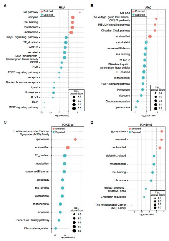
Swann Floc’hlay et al Furlong lab, EMBL

Figure S4: Allelic variation is consistently depleted for transcriptional regulation and enriched
for the expression of metabolic genes
Enrichments for all GLAD categories with statistically significant (p < 0.01, Fisher’s-Exact Test)
enrichment or depletion of significant allelic imbalance for (A) RNA, (B) ATAC or (C-D) histone
modifications. Bubble size represents the number of genes/features per category. For regulatory
elements, category assignments were made on the basis of closest gene annotations.

 4
Floc'hlay_FigS4

Swann Floc’hlay et al Furlong lab, EMBL

 A
 Insecticide
 Aggressive catabolic Response to Response to Response to Response to
 behavior process DTT insecticide mercury ion organophosphorus

 Allelic bias
 general allelic
 Value

 imbalance
 paternally biased
 A

 A

 A

 A

 A

 A
 AC
 AC

 AC

 AC

 AC

 AC

 K4 c
 K4 c

 K4 c

 K4 c

 K4 c

 K4 c
 e3

 e3

 e3

 e3

 e3

 e3
 7a
 7a

 7a

 7a

 7a

 7a
 N

 N

 N

 N

 N

 N
 m

 m

 m

 m

 m

 m
 AT
 AT

 AT

 AT

 AT

 AT
 R

 R

 R

 R

 R

 R
 K2
 K2

 K2

 K2

 K2

 K2

 Data type

 B Chr 2R
 C Genes with
 All genes
 Maternal effects
 ATAC

 Paternal
 Peaks
 Coefficient of genetic variation

 #8332 #8333 #8334
 H3K4me3

 Maternal

 Paternal
 Peaks
 H3K27ac

 Maternal

 Paternal
 Peaks

 Maternal
 RNA

 Paternal
 Genes
 False True False True
 Cyp6g2 Extreme feature Extreme feature
 Cyp6g1
 Enhancers

 r r

Figure S5: Regulatory changes on paternal haplotypes are enriched for genes related to
pesticide resistance and environmental response.
A. Gene categories involved in environmental response and immunity show consistent biases towards
the paternal allele. Coefficients from point-biserial correlation analyses are plotted, with red bars
indicating correlation with the absolute value of allelic imbalance and blue bars (negative values)
indicating correlation with allelic imbalance with the paternal allele being more highly expressed.
B. Cyp6g1, a DTT resistant gene, shows an upregulated paternal allele in every regulatory layer and
in gene expression, with the maternal allele showing no evidence of expression (matching reports in
FlyBase). Grey bars indicate locations of non-uniform mappability across lines. C. Coefficient of
genetic variation for highly imbalanced genes vs. all others (left) or only those with significant line
effects (right).

 5
Swann Floc’hlay et al Furlong lab, EMBL

Figure S6: Time and genotype effect over development
A. Flow diagram showing dynamics of allelic imbalance (AI) in chromatin marks across
developmental time. Proportions of AI and non-AI features are shown in black and grey,
respectively, and represented by the line thickness. Exact proportions for each category are provided
as numbers. B. Histograms showing allelic imbalance for the pde8 gene. Allelic imbalance changes
across time for gene expression level and associated H3K27ac enrichment.

 6
Floc'hlay_FigS7

Swann Floc’hlay et al Furlong lab, EMBL

A B

 ac

 ac

 ac

 ac

 ac

 ac

 ac
 27

 27

 27

 27

 27

 27

 27
 AC

 AC

 AC

 AC

 AC

 AC

 AC
 A

 A

 A

 A

 A

 A

 A
 3K

 3K

 3K

 3K

 3K

 3K

 3K
 N

 N

 N

 N

 N

 N

 N
 AT

 AT

 AT

 AT

 AT

 AT

 AT
 H

 H

 H

 H

 H

 H

 H
 R

 R

 R

 R

 R

 R

 R
 0.96 0.92 0.9 0.91 0.9 0.87 0.93 0.9 0.69 0.93 0.85 0.93 0.87 0.85 0.87 0.9 0.82 0.67 0.83 0.8 0.8
 H3K4me3 0.78 0.54 0.49 0.6 0.55 0.46 0.32 0.15 0.43 0.36 0.07 0.33 H3K4me3 0.4 0.33 0.39 0.74 0.58 0.29 0.52 0.45 0.45
 0.9 0.9 0.85 0.86 0.74 0.8 0.96 0.93
 H3K27ac 0.47 0.49 0.37 0.43 0.34 0.19 0.53 0.32 0.92 0.91 0.76 0.77 0.8 0.81
 0.93 0.95 0.97 0.93 H3K27ac 0.57 0.55 0.45 0.47 0.45 0.46
 ATAC 0.61
 n=20
 0.76
 n=24
 0.65
 n=12
 0.35
 n=12
 0.89 0.87 0.85
 vgn28 vgn57 vgn307 vgn399 ATAC 0.45
 n=21
 0.68
 n=63
 0.57
 n=44

 2-4h 6-8h 10-12h
 0.95 0.89 0.84 0.97 0.89 0.94 0.91 0.92 0.85 0.69 0.84 0.56
 H3K4me3 0.49 0.1 0.09 0.73 0.25 0.49 0.43 0.48 0.17 0.15 0.21 0.36
 H3K27ac
 0.95 0.94 0.91 0.92 0.79 0.88 0.75 0.7 Pearson correlation
 0.52 0.39 0.33 0.38 0.02 0.27 0.03 0.15
 0.95 0.92 0.92 0.74
 ATAC 0.46
 n=12
 0.38
 n=14
 0.47
 n=16
 0.05
 n=18
 -1 -0.5 0 0.5 1
 vgn639 vgn712 vgn714 vgn852

C Alellic ratio Total count

 H3K27ac
 &
 ATAC

 H3K4me3
 &
 ATAC

 H3K27ac
 &
 H3K4me3

 H3K27ac
 &
 RNA

 H3K4me3
 & significance
 RNA FDR > 1%
 FDR < 1%
 RNA
 &
 ATAC
 time point
 0.3 0.0 0.3 0.6 0.0 0.25
 6-8 hr
 partial correlation partial correlation
 10-12 hr
D Alellic ratio Total count 6-12 hr

 H3K27ac
 &
 ATAC

 H3K27ac
 &
 RNA

 RNA
 &
 ATAC

 0.3 0.0 0.3 0.6 0.0 0.25
 partial correlation partial correlation

Figure S7: Partial and Pearson’s correlations on thresholded allelic ratios
A-B. Heatmaps showing the correlation of allelic ratio between each regulatory layer, grouped by
genotype (A) and by time points (B). Values represent the 5% confidence interval for each pairwise
correlation and significant results are emphasized in bold. C-D. Partial correlation results for allelic
ratio and total count values for TSS-proximal (C) and TSS-distal (D) features, grouped by time points.
Whiskers represent the 95% confidence interval ascertained via bootstrapping. See Supplemental
Methods (M3) for the procedure used for thresholding.

 7
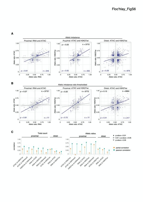
Swann Floc’hlay et al Furlong lab, EMBL

Figure S8: Partial correlation analysis reveals potentially causal relationships among regulatory
layers.
A. Overall Pearson’s correlations in allelic ratios (black values, grey points and regression lines)
between regulatory layers. Correlations are generally modest with little correspondence in allelic
ratios between overlapping non-coding features and associated genes. B. Correlations in allelic ratios
for more imbalanced features (thresholded AI 0.5 +/- 0.06 for all regulatory layers; blue values, points
and regression line) are stronger. C. Comparison between the partial (orange) and the Pearson’s
(blue) correlation for total count (left) and allelic ratios (right). A decrease in partial correlation
denotes a lack of direct relationship within the overall correlations.

 8
Swann Floc’hlay et al Furlong lab, EMBL

Figure S9: Differences in the frequency of cis and trans acting genetic variation among
regulatory layers influences the heritability of regulatory phenotypes
A. For each regulatory layer, cis-trans classified genes/features were assessed to evaluate the relative
contributes of cis and trans to the cis/trans signal. Only RNA has evidence for an unequal
contribution (more trans than cis). B. Scatterplots showing total read counts in the F1 lines vs. the
mean of the two parents for genes/features classified as cis (top) or trans (bottom). Shown in black are
genes/features with an F1 total read count significantly different (FDR
Swann Floc’hlay et al Furlong lab, EMBL

concordance of cis and trans effects suggests predominantly compensatory evolution, while RNA
shows a pattern more consistent with diversifying selection. E. An alternative classification of
selective forces for cis-trans features following Goncalves et al. (2012), which is designed more
explicitly for within species contrasts. As in (d), likely positive selection (cis and trans working in the
same direction) is significantly more common for RNA than for non-coding features.

 10
Swann Floc’hlay et al Furlong lab, EMBL

Supplemental Methods

Fly husbandry, crosses and embryo collection 12
Whole-embryo RNA-seq 13
Whole-embryo ATAC-seq 13
Whole-embryo iChIP 15
Whole embryo gDNA-seq 15
Sequenced reads processing 16
 Personal genome construction 16
 Read mapping 16
 Mappability filter 17
 Quality Control 17
 Peak-calling 19
Total signal quantification 19
 Read assignment 19
 Differential expression across time points 19
 Library size normalization and other processing of total counts 19
Allele-specific signal quantification 20
 Read assignment and gDNA correction 20
 Maternal transcript identification 20
Statistical test for allelic imbalance 21
 Allele-specific changes across lines and developmental time 22
 Gene category enrichment of allelic imbalance 23
Allele-specific changes across regulatory layers 24
 Overlap definition across layers 24
 Partial correlation 26
 Copula directional dependence analysis. 26
 Locus-specific test of gene expression with numbers of open chromatin regions 27
Cis-trans analysis. 27
 Statistical method for steady-state assignment of cis/trans regulatory mechanism 27
 Control for difference in staging between samples 28
Calculating broad sense heritability and coefficient of genetic variation. 29
Measuring additive vs. non-additive heritability 30
The link between trans variation and gene category 30
The impact of cis and trans variation on patterns of selection 31

References 32

 11
Swann Floc’hlay et al Furlong lab, EMBL

Supplemental Methods

Fly husbandry, crosses and embryo collection
 The virginizer line was maintained at 20 ̊C in bottles and flipped once per week. 100-200
adult flies of 5-10 days age were transferred into fresh bottles. The flies were left to lay
embryos for about 24 hours at 20 ̊C before the adults were removed. The bottles were placed
inside a special “heat shocking tray” (a fly tray with holes on the bottom and sides) and the
tray was placed inside a 38 ̊C water bath for 1 hour. After removal from the water bath, the
bottles were kept at 18 ̊C, 20 ̊C or 25 ̊C to synchronize bottles from multiple days. Once the
adult flies eclosed, they were flipped into fresh bottles, to be crossed with the males from the
paternal line later.

 The virgins females that eclosed from the heat-shocked bottles were collected and mated
to males from the paternal lines and placed in collection containers at 25 ̊C two days prior to
embryo collections (Sisson 2007). On the day of collection, three one hour prelays were
performed to stimulate laying, and thereby clear females of any held embryos, followed by 2-
hour collections. The plates with embryos were aged to the appropriate stages at 25 ̊C,
followed by washed into sieves and dechorionated by incubating in 50% bleach for 2.5 min.
The embryos were extensively washed and blotted dry on tissue paper. Approximately 200
embryos were transferred to an eppendorf tube and snap-frozen for subsequent RNA assays.
The majority of embryos were fixed in 1.8% formaldehyde (9.5 ml cross-linking solution
with 485 μl 37% formaldehyde) with vigorous shaking for 15 min at room temperature.
Cross-linking was stopped by incubating with Glycine solution with vigorous shaking for at
least 1 min. After washing with PBT, the embryos were blotted dry. A small aliquot of
embryos (100-200) was transferred into a tube containing 0.5 mL heptane and 0.5 mL
methanol and shaken vigorously for 2 min to devitellinize the embryos. The embryos were
left to settle and liquid was removed as much as possible, followed with 2 washes of
methanol and store at -20 ̊C in methanol for evaluation of the developmental stage of each
collection. The bulk of cross-linked dry embryos were transferred into 1.5 mL eppendorf
tubes, snap-frozen in liquid N2 and stored at -80 ̊C.

 The samples stored in methanol at -20 ̊C were rehydrated at room temperature by
incubating with 50% methanol / 50% PBT for 5 min on a nutator. Nuclei were stained by
incubating the embryos in PBT with DAPI for 5 min on a nutator, followed by washing with
PBT twice. After removing as much liquid as possible, 80% glycerol was added to the

 12
Swann Floc’hlay et al Furlong lab, EMBL

embryos and left to settle in glycerol and then mounted onto a microscope slide, covered with
a cover slip and sealed with transparent nail polish. The developmental stages of the embryo
collection were evaluated by examining the morphological features under the Axio Imager
M2 research microscope (Campos-Ortega 1997).

Whole-embryo RNA-seq
 Embryos were thawed in 200 μl Trizol on ice and smashed with pestle and cordless motor.
Another 800 μl Trizol was added to each sample and samples were shaken by hand for 2-3
min, incubated at room temperature for 5 min. 200 μl of chloroform was added and samples
were vigorously shaken for 30 sec by hand and centrifuged for 15 min at 12,000g at 4 ̊C. The
aqueous phase was transferred to a clean tube and 500 μl isopropanol added to precipitate the
RNA by incubating at room temperature for 10 min, followed by centrifugation for 10 min at
12,000g at 4 ̊C. The RNA pellet was washed twice with freshly made 80% EtOH and
resuspended in 44 μl nuclease-free water. DNA was digested by adding 5 μl DNase 10x
buffer, 1 μl DNase and incubated at 37 ̊C for 30 min. RNA was purified using RNAclean XP
beads. The concentration of total RNA was measured with the Qubit RNA assay kit. If
necessary, the size distribution of the library was checked using RNA 6000 Pico kit on the
Bioanalyzer.

 5 μg of total RNA was taken from each sample and mRNA was extracted using
Dynabeads® mRNA Direct Purification Kit, following the manufacturer’s manual. RNA
tagmentation, reverse transcription, cDNA synthesis and sequencing library preparation were
done using NEBNext Ultra Directional RNA Library Prep Kit following the manufacturer’s
manual.

Whole-embryo ATAC-seq
 Frozen embryos were transferred into a 7 mL douncer placed on ice, thawed in 4 mL HB
buffer supplemented with proteinase inhibitor cocktail cOmpleteTM. Embryos were dounced
20 times with the loose pestle and 10 times with the tight pestle. The homogenate was
filtered through two layers of Miracloth that were positioned 90 ̊ to each other in a clean 15
mL tube. The sample was centrifuged for 7 min at 3500 rpm at 4 ̊C and the murky
supernatant was discarded. The nuclei pellet was resuspended in 3 mL HB buffer and
transferred to a clean 15 mL tube. The nuclei were dissociated by passing them 10 times
through a 20G needle and 10 times through a 22G needle using a 5 mL syringe and then
filtered through 20 μm Nitex membrane on a funnel into a clean 15 mL tube.

 13
Swann Floc’hlay et al Furlong lab, EMBL

 The nuclei extracted were quantified using the LSRFortessa system. 50 μl diluted nuclei
were mixed with 50 μl CountBright Absolute Counting Beads, 197 μl PBS and 3 μl 100x
DAPI and loaded onto the LSRFortessa. The nuclei concentration was calculated as:

55000*(nuclei detected/beads number detected)*dilution factor/50 = nuclei/μl.
 With the quantification of the nuclei solution, we kept 3 aliquots of 200,000 nuclei in 50 μl
PBT for ATAC-seq and 6 aliquots of 40,000 nuclei in 10 μl PBT for iChIP for chromatin
marks. The remaining nuclei were centrifuged at 3500 rpm for 5 min at 4 ̊C, supernatant
discarded, snap-frozen in liquid N2 and stored at -80 ̊C.

 For ATAC-seq, one aliquot of 200,000 nuclei in 50 μl PBT was thawed on ice
supplemented with 50 μl permeabilization solution and incubated on a nutator for 30 min at
4 ̊C. The permeabilized nuclei were centrifuged at 3200 g for 5 min at 4 ̊C and supernatant
removed. The nuclei pellet was resuspended in 50 μl tagmentation mix, containing 5 μl
TDE1, 25 μl 2x tagmentation buffer (both from Nextera kit) and 20 μl nuclease-free water,
and incubated at 37 ̊C for 30 min. 50 μl STOP buffer and 5 μl of 1 mg/mL RNase A were
added to stop the tagmentation reaction and digest RNA by incubating on a thermomixer at
55 ̊C for 10 min with 900 rpm shaking. The reverse cross-linking and protein digestion were
done by adding 3 μl of 20 mg/mL Proteinase K and incubating at 65 ̊C overnight with 900
rpm shaking. The reaction was purified using a MinElute column with Qiagen PCR
purification buffers. The DNA concentration was measured using Qubit. 20 ng of DNA was
brought to 10 μl with water. 2.5 μl i7 primer, 2.5 μl i5 primer, 2.5 μl Nextera primer cocktail
and 7.5 μl Nextera PCR mastermix (all from Nextera kits) were added to complete the PCR
reaction. PCR was run using the following program: 72 ̊C, 3 min; 98 ̊C, 30 sec; cycle start:
98 ̊C, 10 sec, 63 ̊C, 30 sec, 72 ̊C, 3 min, cycle close (run 12 cycles); Hold at 10 ̊C. The PCR
product was run on a 1.2% agarose gel supplemented with 1:20,000 GelGreen for ~50 min at
80V. On the gel, every two samples were separated by one empty lane to avoid cross
contamination. Gel piece from right above the primer dimer band (~100 bp) to 1 kb was cut
with SafeXtractor (one-time use only) on a blue light transilluminator. DNA was extracted
from the gel using Qiagen gel extraction kit and eluted with 2 MinElute columns for each
sample. The concentration of the libraries was measured with Qubit, and the 8 samples were
multiplexed in equal molarity and sequenced on Illumina HiSeq 2500 platform to obtain 125
bp paired-end reads.

 14
Swann Floc’hlay et al Furlong lab, EMBL

Whole-embryo iChIP
 iChIP experiments were performed as described in Lara-Astiaso et al. 2014 (Lara-Astiaso
et al. 2014). In brief, 40.000 D. melanogaster nuclei in a total volume of 10 μl PBS + 0.5%
SDS were used per sample. We usually processed 24 samples in one iChIP experiment. The
nuclei were sonicated in a 0.1 ml sonication tube (Diagenode Cat. No. C30010015) at 4°C for
40 cycles 30’’/30’’ ON/OFF using the Bioruptor Pico (Diagenode). For the first IP,
Chromatin was immobilized with 1.3 μg of anti-H3 antibody (abcam ab1791) and Dynabeads
Protein G (Invitrogen, Cat. No. 10003D) on a rotating wheel overnight at 4°C. Following
Chromatin End Repair and A-tailing, the samples were indexed by ligation of Y-shaped
Index Adaptors containing P5 and P7 sequences.

 After Chromatin Release, samples were pooled by 8, resulting in three pools. These pools
were split into two second IPs each. The chromatin was incubated at 4°C for 3h on a rotating
wheel with 2.5 μg of antibody against H3K27ac (abcam, ab4729) or H3K4me3 (Millipore,
07-473), followed by a 1 h incubation with Dynabeads Protein G. The IPs were washed, the
ChIPed DNA was eluted and purified. For Library Amplification, KAPA HiFI Hot Start
Ready Mix (KAPA Biosystems, KM2605) and primers containing the Illumina P5-Read1 and
P7-Read2 sequences were used. After a final clean-up with AmPure XP beads (Beckman,
Cat No. 63880), the quality of the libraries was determined by qPCR. To assess efficiency
and specificity of the ChIP, we used a positive and a negative target region and compared the
enrichments by qPCR before and after library amplification. The libraries were run on a
Bioanalyzer chip, multiplexed and sequenced with Illumina NextSeq500 high 150bp PE.

Whole embryo gDNA-seq
 We isolated gDNA from ~100 embryos per F1 cross using an electric pestle and Solution
A from Qiagen (0.1mM Tris-HCl pH9.0 / 0.1 M EDTA / 1% SDS). Following this step, the
lysate was incubated for 30 min at 65˚C followed by the addition of 28 μl 8M KAc and
30min incubation on ice. The debris was then spun down and the supernatant cleaned up
using a standard Phenol/Chloroform extraction. The resulting gDNA was processed in a
75bp SE sequencing library using NEBNext DNA Ultra 2 protocol on a Hamilton automated
Liquid Handling system and sequenced on an Illumina NextSeq.

 15
Swann Floc’hlay et al Furlong lab, EMBL

Sequenced reads processing

Personal genome construction
 As a starting point for all personal genomes, we began with Drosophila reference
assembly dm3 as downloaded from the UCSC genome browser (version 5 from FlyBase)
along with reference annotations r5.57 from FlyBase. To generate reference genomes for our
paternal lines, we downloaded variant calls for the full 205 lines of the DGRP
(http://dgrp2.gnets.ncsu.edu/) made against the dm3/v5 D. melanogaster reference genome.
For each paternal line from DGRP, we inserted SNPs and indels from the VCF file into the
reference genome. Changes in coordinates were recorded in a liftOver chain file for
subsequent steps. Heterozygous SNPs were replaced with the appropriate ambiguity code
with missing data (‘.’) recorded as an N. Heterozygous indels were inserted as a string of N
equal to the length of the longer haplotype. In the case of the Virginizer line, we made use of
a VCF file generated for reference genome dm6/v6 (Ghavi-Helm et al. 2019) and converted
the coordinates to dm3 using pslMap (http://genome.ucsc.edu/, v5). The same steps for
reference generation was used for the DGRP paternal lines. For all parents, a genotype-
specific set of annotations was created using liftOver to translate the r5.57 reference GFF3
file into the coordinate frame of the custom parental genome.

Read mapping
 Read were trimmed for adaptor sequences and sequencing quality using skewer (v0.2.2)
and seqtk (v1.0), respectively, with default parameters. To avoid mappability bias, we used
the parental genome mapping strategy (see mappability filter section, below) and mapped
reads to both personalized parental genomes (Skelly et al. 2011). Reads from ATAC-seq and
ChIP-seq were mapped using BWA (v0.7.12) (Li and Durbin 2010), reads from RNA-seq
were mapped using STAR (v2.5.1b) (Dobin et al. 2013) and FlyBase gene annotation version
5.57. Aligned reads were clipped when overlapping their read pairs using clipOverlap
(v1.0.14). Using the appropriate chain files and pslMap (http://genome.ucsc.edu/), alignment
coordinates were converted into the reference Drosophila melanogaster r5.57 genome
coordinate space, also used in the DGRP project for variant calling.

 Resulting alignments from both parental genome mappings were merged into a single
alignment file, where reads aligned in both cases were reported only once (selecting the
alignment with the highest mapping score).

 16
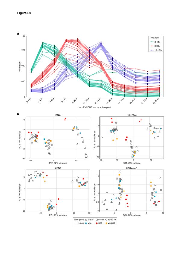
Swann Floc’hlay et al Furlong lab, EMBL

Mappability filter
 To ensure equal mappability across the two parental genomes for a given F1 line, we made
use of two approaches. First, genomic DNA sequencing data from all the parental lines were
mapped using STAR on their personalized genome and converted into the r5.57 reference
using pslMap (http://genome.ucsc.edu/). Coverage data was produced using pslToBed
(http://genome.ucsc.edu/) from the UCSC genome browser utilities. For each of our F1
crosses, genomic regions showing a null coverage in either the mother or the father line were
discarded from the analysis by trimming the portion of the aligned reads overlapping such
regions. Second, for each of the parental genotypes, we simulated transcriptomic and
genomic reads spanning the entire genome with equal coverage (one read starting at each
base pair, read length=100bp). The resulting reads were mapped on the corresponding
parental genome and converted to the reference genome coordinates in the same manner as
the RNA-seq, ATAC-seq and ChIP-seq experiments. For each of the F1 lines, regions
showing a different coverage between the paternal and maternal synthetic read mapping were
not considered when calling allele-specific measures. This step captured mappability issues
caused by ambiguous bases and Ns introduced during the construction of the parental
reference genomes. In order to compare total coverage measures across samples, a universal
mappability filter encompassing all the line-specific filtered regions was applied to trim the
reads before further analysis.

Quality Control
 We evaluated the quality of our sequencing data in three ways. First, we looked at
pairwise correlations between each sample. We observed a Spearman’s correlation of at least
0.95 in all biological replicates (Supplemental Fig. S1b), while the median Spearman’s
correlations between samples from different genotypes or different time points were lower, as
expected, ranging between 0.84 and 0.98 for all data types (Supplemental Fig. S1c). Second,
we performed a principal component analysis at the level of total counts to look for evidence
of issues for specific samples (e.g. failure to cluster with a replicate or clustering with the
wrong time point). Third, in the case of RNA, we looked for correlations between our
samples and the modENCODE time series of development (Supplemental Fig. M1, below)
(Graveley et al. 2011). Through these last two steps, we realized significant issues with the
6-8hr time point for the parental line 399 – while the replicate correlations are high, these
samples appear closer to 10-12hr than they do 6-8hr. We thus removed these two samples

 17
Swann Floc’hlay et al Furlong lab, EMBL

from all analyses, reducing our cis/trans analyses for RNA to only the 10-12hr time point.
No similar staging issues are apparent in the open chromatin or histone modification data.

Figure M1: Total count data cluster with similar time points
a. Correlation of gene expression total count data with modENCODE time series. As expected, the
highest correlation corresponds to the comparison with equivalent time points. b. Principal
component analysis of total count data for each data type. Parent-offspring trio is shown in color. For
gene expression data (upper, left), the two replicates of parental line 399 at 6-8hr cluster together with
the 10-12hr samples. We removed these samples from further analysis.

 18
Swann Floc’hlay et al Furlong lab, EMBL

Peak-calling
 For ChIP-seq experiments targeting H3K4me3 and H3K27ac marks, peak calling was
performed for each sample on each parental genome using Macs2 (v2.1.1) (Zhang et al.
2008) with the broad option and default parameters. After converting all peak calls to the
dm3 coordinates, we merged peaks using the bedtools merge function to produce a single
peak set used across all lines and all developmental time points (Quinlan and Hall 2010). For
ATAC-seq experiments, regions of chromatin accessibility were defined as the merge of peak
summits called by Hotspot (v4.0.0) (John et al. 2011), with a score higher than 5 in at least
one of the F1 samples after extending the summits by 200bp in both directions.

Total signal quantification
Read assignment
 For each individual sample, total coverage signal was evaluated at the feature level (genes
or peaks) using scripts accessing the pysam package (Li et al. 2009). Each read mapping to
at least one of the two parental genomes and not filtered by the mappability filter was
assigned to its overlapping feature. Reads not overlapping a SNP were also included in this
process, as this measure is not allele-specific.

Differential expression across time points
 To quantify changes in total read counts between time points, we imported the total count
data into DESeq2 and fit a model consisting of line + time (Love et al. 2014). For any gene
with a significant (FDR < 0.1) time effect, we subsequently looked for evidence of changes
between neighboring time points using the contrasts option in DESeq2. One concern is that
some genes may have expression levels that are simply too low to provide statistical power.
To avoid this issue, we presented results only from genes whose mean expression across all
three time points was equal or greater to the read count threshold identified via DESeq2
implementation of independent filtering (Bourgon et al. 2010).

Library size normalization and other processing of total counts
 Upon visual inspection of the total count distribution across data types, we set the
minimum of 20 reads per feature as the threshold for detecting expressed genes and non-
coding peaks. Total counts were library scaled and TMM normalized using EdgeR
(Robinson et al. 2010). Values are expressed in log10 (Counts Per Million).

 19
Swann Floc’hlay et al Furlong lab, EMBL

Allele-specific signal quantification

Read assignment and gDNA correction
 For each dataset, allele-specific counts were performed at the feature level, i.e. per genes
for RNA-seq and per peak for ATAC-seq and ChIP-seq. Based on their genotype at the SNP
location, reads overlapping a feature were assigned to the maternal or paternal haplotypes.
Reads not overlapping a segregating SNP or reads with disagreeing assignment between
SNPs were ignored in the measurement. Cases of genotyping errors can potentially lead to
incorrect allelic imbalance measure if a SNP is wrongly called as segregating in a given
cross. To correct for these events, we performed a genomic DNA-seq experiment for each of
the F1 lines and processed it in the same manner as the ATAC-seq data. Using a two-sided
binomial test with false discovery rate correction, we tested for each SNP whether the
number of reads assigned to the maternal and the paternal haplotypes were significantly
different from an expected 50:50 ratio in the autosomes. In chrX, the expected ratio was
empirically measured from the 1000 SNPs with the highest coverage in chrX. Only SNPs
with a minimum coverage of 15 reads for autosomes and 10 reads for chrX were tested.
SNPs considered as significantly imbalanced (p < 0.05) for the genomic DNA data were
formatted as missing data (N) for alignment and were ignored when performing the allele-
specific measures. In order to evaluate the sex ratio of our pool of embryos, allele-specific
counts of gDNA reads were also performed at the feature level.

Maternal transcript identification
 Due to the presence of maternally deposited transcripts, especially in the early 2-4hr time-
point, a portion of the genes has an allelic imbalance biased toward the mother in the RNA-
seq data. In order to detect them, we used RNA-seq data from unfertilized eggs from the
same developmental time windows as the F1 samples. To identify genes with maternal
deposition, we plotted the log10 read count of each gene as measured in freshly laid eggs (the
first time window), and used the bimodality of this distribution to set a threshold for
“expressed”. The majority of these genes were excluded from subsequent analyses.
However, as previously noted (Thomsen et al. 2010), we observed a population of these
transcripts that decayed over time, becoming not detected by 6-8 hours. Formally, we
quantified this population as those transcripts showing significant evidence of decay (using
DESeq2) between 2-4h and 10-12h (Supplemental Fig. M2, below). As this population of
transcripts shows a 50:50 autosomal ratio in the 6-8h and 10-12h datasets, we included them
in our analyses.

 20
Swann Floc’hlay et al Furlong lab, EMBL

In addition to maternal transcript removal, as we used a poly(A)+ selection step in the
construction of our RNA-seq libraries, any genes that largely or entirely lack polyadenylation
signal (e.g. ncRNA, snRNA, rRNA) were removed from our analyses categories.

Figure M2: Maternally deposited transcripts show different rates of decay
 Distribution of allelic ratios for gene expression data for line vgn28 at each time point. The genes are
separated into three categories, based on their expression in freshly laid eggs (i.e. purely maternally
deposited transcripts). Left: genes detected in unfertilized eggs (maternal transcripts) showing no
evidence of decay at 10-12h. Middle: genes detected in eggs and showing significant decay between
2-4hr and 10-12h. Right: genes not detected in eggs, only zygotically expressed. Zygotic genes and
maternally deposited genes with evidence of fast decay are included in the analysis.

Statistical test for allelic imbalance
Individual tests were performed for each line and for each time point. Total F1 counts
( !",$,% can be modeled on an allele-specific basis ( !",$,% ) using a beta-binomial distribution.

Specifically, !",$,% denotes the number of reads from the maternal allele mapped to feature f

for pool of individuals i, of paternal strain s, at time t. !",$,% denotes the total number of reads
mapping to genes for pool of individuals i of strain s, at time t.

 &",$,% ~ ( &",$,% , &",$,% )

 !",$,% ~ ( , )

where , are the shape parameters of the beta distribution. We tested the following
scenarios by maximum likelihood estimation:

 : =

 : ≠

 21
Swann Floc’hlay et al Furlong lab, EMBL

Due to limited replicates per condition, we used information across features to reduce the
uncertainty of estimates and improve power by assuming that all features have the same
mean-variance relationship (Robinson et al. 2010; Love et al. 2014). Empirical data was used
to estimate the over-dispersion parameter ( ) for each data type based on the beta-binomial
distribution. Maximum likelihood estimation was used to obtain and for each feature of
time t and strain s. is calculated as follows:

 1
 =
 + +1

The mean over-dispersion value for all features was used as the shrinkage term and likelihood
ratio tests (df=1) were used to obtain a p-value, which was adjusted using FDR (Benjamini
1995). Autosomes were tested separately to sex chromosomes; features on the X
Chromosome were tested using a background allelic ratio of no imbalance centered on the
averaged ratio of maternal versus paternal alleles across the data set being compared (i.e.
RNA, ATAC, H3K4me3, H3K27ac). Autosomal features were tested using a null
distribution of 0.5.

Allele-specific changes across lines and developmental time
 We use a linear mixed-effects model where a random effect is incorporated to estimate
variability between strains. Specifically, &'"( represents the proportion of reads
 )*%+(,*-
)*%+(,*-./*%+(,*-
 , mapped to a feature f in data type d of strain s, replicate r and time t.

Random effect components were incorporated to estimate variability between pools of
individuals, time points and lines.

 &',",(,% = & + &% + &" + ( )%& &" ~ Ν(0, &0 )
 & is the intercept term. &% is a random effect term denoting time. &" is a random effect
based on strain and ( )%& is a interaction term for time by strain.
 1 : & ≠ 0, &% ≠ 0, &" ≠ 0, ( )%& = 0
 2 : & ≠ 0, &% = 0, &" ≠ 0, ( )%& = 0
 0 : & ≠ 0, &% ≠ 0, &" = 0, ( )%& = 0
 3 : & ≠ 0, &% ≠ 0, &" ≠ 0, ( )%& ≠ 0

To infer the significance of time or strain dependent allele bias, we restrict the values that the
parameters can take where 1 is the full model that controls for effects due to time, genotype

 22
Swann Floc’hlay et al Furlong lab, EMBL

as well as the time by genotype effect. 2 is a model where we assume no allelic balance
between time points after controlling for strain effects. Conversely, 0 accounts for allelic
imbalance changes by time points while controlling for strain effects. 3 specifies a non-
zero interaction term between time and line. Each model is fitted to the data in turn by
maximizing the likelihood using the R library ‘lme4’ (Bates 2015). Akaike information
criterion (AIC) is used to assess the best model.

 Prior to analysis, count data filtered for reads with more than 20 allele-combined counts.
Additionally, maternally deposited genes were removed for gene expression counts, as
described above. For this analysis, the sex chromosome was removed. Each feature is tested
using read counts at SNPs common to all lines.

Gene category enrichment of allelic imbalance
 To better understand the biological functions affected by cis-regulatory variation, we
looked for the enrichment/depletion of allelic imbalance in functional categories using a
Fisher’s exact test. We focused on the gene-centric GLAD categories (Hu et al. 2015), which
are broadly representative of the trends observed using other ontologies (Supplemental Table
S5). In these analyses, chromatin features (ATAC and histone mark peaks) were assigned to
the closest gene, though similar results were obtained if we limit our analysis to only
promoter-proximal elements (
Swann Floc’hlay et al Furlong lab, EMBL

Allele-specific changes across regulatory layers

Overlap definition across layers
 Each set of non-coding features were split into TSS-distal and TSS-proximal subsets.
Features are considered as part of the TSS-proximal set if their nearest TSS is not further than
500bp away or if they overlap a region called as a H3K4me3 peak. For each subset, we
defined regions of overlap between the regulatory layers as the overlap portion of two or
more non-coding features. In the case of the overlap of three features, at least one base pair
must be shared with all the layers to create an overlap.

 For the proximal subset, genes features are assigned to a given overlap region if the
distance between the overlap boundaries and the TSS is smaller or equal to 500bp. For the
distal subset, overlaps are associated with the gene having the closest TSS. To avoid mis-
assignment of TSS to proximal cis-regulatory overlaps, we excluded TSS positioned in the
600bp upstream region of other TSS.

 During our partial correlation (and related) analyses, as we noticed a clear drop in the
correlation between the regulatory layers when the distance between the nearest TSS and the
chromatin features exceed 1500bp (Supplemental Fig. M3a, below), we thus restricted the
TSS-distal set to a maximum distance to TSS of 1500bp.

 The characterization of overlapping regions (i.e. regions of overlap between multiple non-
coding features) resulted in the definition of TSS-distal ATAC-only and H3K27ac-only
peaks, which did not overlap each other (Fig. 1c). We assessed the enrichment for regulatory
signatures and transcription factor binding motifs of these peak sets using i-cisTarget
(Imrichova et al. 2015) and RSAT (Nguyen et al. 2018) (Supplemental Table S3). Strong
enrichment for Polycomb and Su(Hw) ChIP-seq signal was observed in ATAC-only peaks
(NES > 5), which was further supported by the enrichment for Su(Hw) binding motif in the
de-novo motif discovery analysis (e-value = 3 x 10-11). In H3K27ac-only peaks, strong
enrichment for Polycomb, Elav and H3K27me3 ChIP-seq signal was observed (NES > 5).

In both ATAC-only and H3K27ac-only peaks sets, an enrichment for RNA polymerase II
ChIP-seq signal was also observed (mean NES of 10.26 and 6.02 for ATAC-only and
H3K27ac-only peaks, respectively), although it did not reach the enrichment score observed
in the overlapping peaks (mean NES = 10.81 and 10.2 for ATAC & H3K27ac overlapping
peaks, respectively).

 24
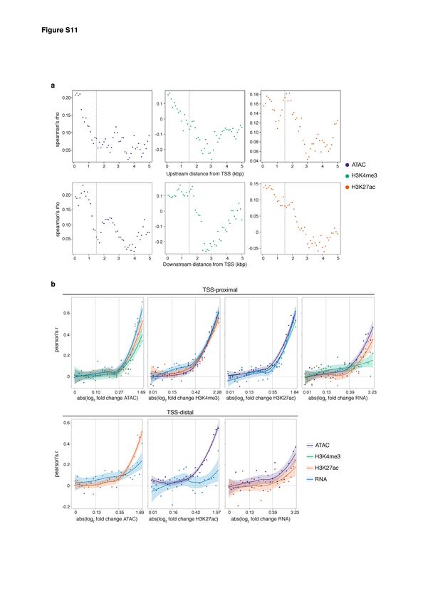
Swann Floc’hlay et al Furlong lab, EMBL

Figure M3: AI and TSS distance thresholding increases correlation between regulatory layers
a. Spearman’s correlation of allelic ratios between genes expression and the other regulatory layers,
as a function of their distance from TSS. Correlations are shown for non-coding features located from
0 to 5kb upstream (upper row) or 0 to 5kb downstream (lower row) of the TSS. As the correlation
values show a clear drop for distances further than 1.5kb, we removed features greater than 1.5kb
from TSS (upstream and downstream) from the TSS-distal overlap set. b. Pearson’s correlation of
allelic ratios between regulatory layers for TSS-proximal (upper row) and TSS-distal (lower row)
features at 10-12hr. Correlations are binned into 30 quantiles based on the absolute log2 fold change
of allelic ratio. Values on x-axis show the mean log2 fold change in the 1st, 10th, 20th and 30th
quantiles from left to right. Shaded regions indicate the 90% confidence intervals. In most cases, we
see an inflection point around the 18th quantile, which was used to set the AI threshold of 0.5 +/- 0.06
in further analysis.

 25
Swann Floc’hlay et al Furlong lab, EMBL

Partial correlation
 Partial correlation analysis was performed using the R package ‘GeneNet’ (Opgen-Rhein
and Strimmer 2007) for both allelic ratios and total count data and for TSS-proximal and
TSS-distal sets (excluding the X Chromosome). We used features with no missing data in
any of the regulatory layers (Supplemental Fig. S8). For allelic ratio data, we observed a
distinct increase in Pearson’s correlations between layers as the AI fold change increased,
suggesting a threshold below which allelic imbalance was effectively “noise”. To establish a
filtering threshold for “noisy” allelic imbalance, we separated each dataset into 30 bins of
total allelic imbalance and plotted the average correlation in allelic fold change between
datasets for each bin (Supplemental Fig. M3b, above). In each case, there is a general
inflection point in the correlation at an allelic ratio of ~0.5 +/- 0.06. We filtered loci that fell
below this threshold to improve the covariance signal of AI datasets for partial correlation
analysis (Supplemental Fig. S8).

 For both TSS-proximal and TSS-distal analysis, the Pearson’s and the partial correlation
results are largely consistent between time points and genotypes (Supplemental Fig. S7).
Samples from different time points and genotypes were thus pooled for this analysis.
Because the different ratios for autosomes and X Chromosomes would lead to an artificially
inflated correlation, X Chromosome genes/features were removed for this analysis. We
additionally performed bootstrapping over 2000 iterations and 80% sampling to compute
confidence intervals (Supplemental Fig. S7).

Copula directional dependence analysis
 Directional dependence modeling was done in a regression framework using copulas to
describe the bivariate distribution between our pairwise datasets. A copula is a multivariate
distribution where the marginal distributions are uniform (Sklar 1973; Kim 2017). Any
multivariate function, F(x,y), can be represented in a copula as a function of its marginals,
C( 4 ( ), 5 ( )). Hence, given two random variables X and Y, the copula C(u,v) reflects this
dependency, and = 4 ( ), = 5 ( ) are the marginal variables with uniform
distributions. Given an asymmetric copula, it is possible to infer directional dependence
based on the proportion of total variance of V that can be explained by the copula regression
 6|8 ( ) compared to the proportion of total variance of U that can be explained by the copula
regression 8|6 ( ) (Sungur 2005; Lee and Kim 2019). We use the method of Lee and Kim
2018 (Lee and Kim 2019) to infer the flow of information for pairwise relationships that

 26
Swann Floc’hlay et al Furlong lab, EMBL

showed a significant relationship in partial correlation analyses. Analyses were performed
for allele-specific and total counts and at different developmental time points (excluding 2-
4hr and sex chromosomes). X Chromosome data was kept for both analyses and it removal
did not change the direction of findings but did increase effect size.

Locus-specific test of gene expression with numbers of open chromatin regions
 ATAC-seq peaks were associated to genes at +-1500bp from the TSS and the relationship
between the regulatory datasets was tested on a locus-specific basis. We note that the results
obtained from this analysis, showing less imbalance in expression with more local peaks, are
unlikely to be due to differences in statistical power, as genes linked to shadow enhancers and
multiple peaks are typically more highly expressed (wilcox test, p < 1.5 x 10-69). Hence,
there is greater power to detect allelic imbalance.

Cis-trans analysis

Statistical method for steady-state assignment of cis/trans regulatory mechanism
 For one F1 line (vgn x 399), we use maximum likelihood estimation (MLE) to compare
parental and offspring ratios simultaneously to determine whether gene expression, chromatin
accessibility, H3K4me and H3K27ac enrichments are influenced by cis-, trans, conserved or
both cis- and trans- acting effects by modeling read counts in parents using negative binomial
distributions and the F1 alleles using beta-binomial distribution. We then find the most likely
model for each gene.

 For each gene, F0 counts from each strain can be modeled as a negative binomial marginal
distribution, while F1 counts were modeled using a beta-binomial distribution where the
parameters of the beta distribution modeled the proportional contribution from each allele.
For each data type, there were 2 replicates (i) for each F0 strain and 2 replicates (j) for F1
samples. F0 counts for each strain ( $ , and $ ) were assumed to follow negative binomial
distributions while F1 counts ( 9 ), were modeled on an allele-specific basis ( 9 ) using a beta-
binomial distribution:

 $ ~ ( $ ), $ ~ ( $ ), 9 ~ ( 9 , 9 ) (1)
 ; <
 $ ~ Q , S , $ ~ T , U , 9 ~ ( , ) (2)
 1 − ; 1 − <

 27
Swann Floc’hlay et al Furlong lab, EMBL

where $ is formally defined as the count of the variant in the ith vgn F0 line, $ is the
binding intensity of the variant in the ith dgrp399 F0 line, 9 is the number of reads mapping
across both allelic variants in the jth F1 hybrid and 9 is the number of reads mapping to the
vgn allele in the jth F1 hybrid.

 We estimate the dispersion parameter r for F0 samples using the ‘estimateDispersions’
function within ‘DESeq2’ with local regression fit. r was used as the reciprocal of the fitted
dispersion value from ‘DESeq2’.

 We constrained parameter estimation for each distribution based on four different
regulatory scenarios and derived maximum likelihood values for each hypothetical case on a
site-by-site basis. The four models are described below:

 : ; = = =
 ;
 1 − ;
 : ; ≠ = = ; <
 + +
 1 − ; 1 − <

 : ; ≠ = =
 : ; ≠ = ≠

 Figure 6c, showing the proportion of features assigned to each category, we presented the
maximum likelihood assignment. In subsequent analyses, we limited our analyses to features
that showed a BIC difference ≥ 2.

 For the cis and trans assignments, we focused only on autosomal features. This was in
part due to the complications of calculating cis/trans components for two different sets of
expected ratios, but also because the difference in expected ratio between the X Chromosome
and the autosomes can influence the power to detect allelic imbalance and, thus, influence the
assignments of cis vs. trans, with resulting complications for downstream analyses (e.g.
categorical enrichment)

Control for difference in staging between samples
 A challenge in assessing cis and trans proportions during development is the influence of
differences in staging between samples, which can induce differences in read counts that will
not be reflected in allelic ratios. If these differences stem from genetically based differences
in developmental rates, then the classification would reflect genuine trans differences.

 28
Swann Floc’hlay et al Furlong lab, EMBL

Environmental variation or differences in sample handling, however, can also lead to
developmental shifts. To evaluate this possibility, we looked first to see if genes and features
classified for trans frequently showed evidence of an increase in log2 fold-changes between
time points. For all regulatory layers, we observed a significant increase in log2 fold-changes
between time points for genes and features classified as trans (p < 2.2 x 10⁻¹⁶). However, we
see no evidence for a coordinated shift in the parental ratios used to calculate trans relative to
log2 fold-changes between time points. Indeed, genes and feature counts that increase during
development are equally likely to show higher expression in either the maternal line (vgn) or
paternal line (DGRP-399). We thus conclude that while a portion of our observed trans
effects may result from differences in developmental timing, the majority are likely genetic in
origin, as global shifts in developmental staging (e.g. from handling errors or differences in
collection temperature) would induce clear correlations between log2 fold-change over
development and expression bias towards the more developmentally advanced parent.

Calculating broad sense heritability and coefficient of genetic variation
 To avoid potential interaction effects with ‘time’, we fit a separate model for each time
point (all three time points in the case of the chromatin data, and excluding 2-4h in the case
of RNA). For each gene/feature, we used the lmer function from lme4 to estimate a random
effect for line after applying the vst function in DESeq2 to bring the trait values more closely
in line with normality. To evaluate the significance of the resulting fit, the model was
compared to a null model consisting only of an intercept using the anova function. FDR
values were calculated from the resulting vector of p-values using the qvalue function in R
(v3.5.1). Estimated line variances and residual variances were extracted from the model using
the ‘VarCorr’ function. Line variances were treated as proportional to broad-sense
heritability (H^2). We calculated the coefficient of genetic variation by scaling our estimated
‘between-line variances’ by the variance stabilized mean read count of each feature such that
genetic variation is presented as a percentage deviation from the average of the population
(Berney et al. 1975; Garfield et al. 2013). We used the formula below:

 √
 = 100 ×

In our analysis, H^2 and coefficient of genetic variation were considered meaningful as long
as the line-model was significant with an FDR < 0.1.

 29
Swann Floc’hlay et al Furlong lab, EMBL

 The result of the above process generated one value per time point for each feature. An
alternative is to fit a similar model to the above for all times (excluding 2-4h in the case of
RNA) and including a term for ‘time’. The resulting distributions for H^2 and coefficient of
genetic variation were qualitatively similar. The enrichment calculations were carried out as
described above.

Measuring additive vs. non-additive heritability

In the case of additively inherited gene expression (or read counts for any of our measured
features), the signal observed in the F1 is expected to be equal to the midpoint (average) of
the two parents, while non-additively inherited genes/features should show a significant
departure from that midpoint. To formally test for non-additivity, we made use of the
standard workflow in DESeq2 with two modifications. First, we set the betaPrior option
equal to TRUE. After setting the reference genotype to the F1 (vgn x 399) using the relevel
function, we then extracted the results using the ‘results’ function and the contrast vector
c(0,1,-.5, -.5) to contrast the full value of the F1 genotype with ½(vgn + 399). Features with
an FDR < .1 were considered as “non-additive”.

The link between trans variation and gene category

 Mirroring our buffering results, genes with more regulatory elements in their vicinity are
more likely to be classified as trans-acting having more peaks in their immediate regulatory
domain (trans = 2.58 peaks per gene vs. 1.9, p = 0.00094). Similarly, there is a significant,
though modest, enrichment of trans influences among TFs and a depletion among metabolic
genes, two categories that are strongly distinguished in the complexity of their associated
regulatory landscapes (Supplemental Table S9). This appears to have downstream impacts
on the heritability of gene expression for different gene categories. Among 80 tested gene
categories, DNA-binding TFs (p = 3 x 10⁻³) and interestingly mitochondrial associated genes
(p = 2 x 10⁻⁶) stand out as the two gene categories with statistically elevated frequencies of
non-additive inheritance (Fisher’s exact test; Methods). Thus, while TFs generally show
reduced genetic variation among lines and reduced allelic imbalance in gene expression
(Supplemental Fig. S4), they are still affected by trans-acting variants whose non-additive
inheritance reduces the efficacy by which selection can alter gene expression differences
among different lines.

 30
Swann Floc’hlay et al Furlong lab, EMBL

The impact of cis and trans variation on patterns of selection

Genes influenced by both cis and trans acting variants (cis-trans) provide an opportunity to
understand patterns of recent selection: In the face of compensatory evolution, cis and trans
acting influences are more likely to work in opposite directions, while directional selection
will be more likely to reinforce cis and trans effects acting in the same direction. Using the
classification of cis and trans by Goncalves et al (Goncalves et al. 2012)(see below), we
observed that cis and trans effects were much more likely to act in a compensatory manner as
compared to gene expression: for chromatin accessibility and histone modifications, 13% of
cis-trans features were classified as same vs. 37% for RNA (Fig. 6c: p < 2.2 x 10⁻¹⁶ chi^2).
This suggests that for RNA there is either more frequent directional selection or less efficient
selection against directional changes. This result is robust to the method used to classify cis
+ trans effects (Landry et al. 2005), with 63% of cistrans RNA features being classified as
divergent for RNA vs. 22% for chromatin features (Supplemental Fig. S9d: p < 2.2 x 10⁻¹⁶;
chi^2). Taken together, these results suggest clear differences in evolutionary trajectory
between regulatory layers which reflects population processes operating at different levels of
organization, as well as differences between functional gene classes. The classification of
Goncalves et al. (Goncalves et al. 2012) is as follows. For all genes, we asked if their cis and
trans contributes act to reinforce one another (same direction) or if they operated in opposite
directions. Formally, for the i_th gene, we define the average log2 fold change for the
parental lines as x_i and the average log2 allelic ratio from the F1 data as y_i. We then
classified:

Opposite – cis stronger: (0 < y_i < x_i) OR (0 > y_i > x_i)

Opposite – trans stronger: (x_i < 0 < y_i) OR (y_i < 0 < x_i)

Same – cis stronger (0 < x_i < y_i < 2x_i) OR (0 > x_i > y_i > 2x_i)

Same – trans stronger (0 < 2x_i < y_i) OR (0 > 2x_i > y_i)

 31
You can also read