SUBDUCTION EARTHQUAKES CONTROLLED BY INCOMING PLATE GEOMETRY: THE 2020 M 7.5 SHUMAGIN, ALASKA, EARTHQUAKE DOUBLET - EARTHARXIV
←
→
Page content transcription
If your browser does not render page correctly, please read the page content below
Subduction earthquakes controlled by incoming plate
    geometry: The 2020 M>7.5 Shumagin, Alaska,
                  earthquake doublet
                  Yu Jianga, Pablo J. Gonzáleza,b, Roland Bürgmannc
        aCOMET,   Department of Earth, Ocean and Ecological Sciences, School of
    Environmental Sciences, University of Liverpool, Liverpool, L69 3BX, United Kingdom,
                                   Yu.Jiang@liverpoolac.uk
      bVolcanology Research Group, Department of Life and Earth Sciences, Instituto de

Productos Naturales y Agrobiologıa (IPNA-CSIC), 38206 La Laguna, Tenerife, Canary
                        Islands, Spain, pabloj.gonzalez@csic.es
cDepartment of Earth and Planetary Science, University of California, Berkeley, CA,

                         USA, burgmann@seismo.berkeley.edu

This manuscript is a preprint and has been submitted for publication in Earth and Planetary
Science Letters. Please note that the manuscript is undergoing peer review and has not
been accepted for publication. Subsequent versions of this manuscript may have slightly
different content. If accepted, the final version of this manuscript will be available via the
Peer-reviewed Publication DOI link on the right-hand side of this webpage. Please feel free
to contact the corresponding author; we welcome feedback.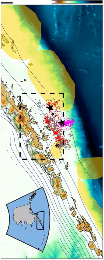
Subduction earthquakes controlled by incoming plate
    geometry: The 2020 M>7.5 Shumagin, Alaska,
                  earthquake doublet
             Yu Jianga , Pablo J. Gonzáleza,b , Roland Bürgmannc
        a
          COMET, Department of Earth, Ocean and Ecological Sciences, School of
 Environmental Sciences, University of Liverpool, Liverpool, L69 3BX, United Kingdom
b
  Department of Life and Earth Sciences, Instituto de Productos Naturales y Agrobiologı́a
            (IPNA-CSIC), 38206 La Laguna, Tenerife, Canary Islands, Spain
  c
    Department of Earth and Planetary Science, University of California, Berkeley, CA,
                                          USA

Abstract

In 2020, an earthquake doublet, a M7.8 on July 22nd and a M7.6 on Octo-
ber 19th, struck the Alaska-Aleutian subduction zone beneath the Shumagin
Islands. This is the first documented earthquake doublet, of considerable
size, involving a megathrust event and a strike-slip event, with both events
producing deeply buried ruptures. The first event partially ruptured a seis-
mic gap, which has not hosted large earthquakes since 1917, and the sec-
ond event was unusual as it broke a trench-perpendicular fault within the
incoming oceanic slab. We used an improved Bayesian geodetic inversion
method to estimate the fault slip distributions of the major earthquakes us-
ing Interferometric Synthetic Aperture Radar (InSAR) wrapped phase and
Global Navigation Satellite Systems (GNSS) offsets data. The geodetic in-
versions reveal that the Shumagin seismic gap is multi-segmented, and the
M7.8 earthquake ruptured the eastern segment from 14 km down to 44 km
depth. The coseismic slip occurred along a more steeply, 26-degree dipping

Preprint submitted to Earth and Planetary Science Letters                  May 16, 2021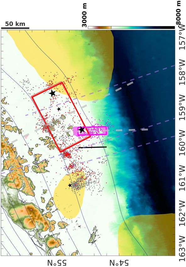
segment, and was bounded up-dip by a bend of the megathrust interface to
    a shallower 8-degree dip angle connecting to the trench. The model for the
    M7.6 event tightly constrained the rupture depth extent to 23-37 km, within
    the depth range of the M7.8 coseismic rupture area. We find that the M7.6
    event ruptured the incoming slab across its full seismogenic thickness, po-
    tentially reactivating subducted Kula-Resurrection seafloor-spreading ridge
    structures. Coulomb stress transfer models suggest that coseismic and/or
    postseismic slip of the M7.8 event could have triggered the M7.6 event. This
    unusual intraslab event could have been caused by accumulation and lo-
    calization of flexural elastic shear stresses at the slab bending region. We
    conclude that the segmented megathrust structure and the location of in-
    traslab fault structures limited the rupture dimensions of the M7.8 event
    and are responsible for the segmentation of the Shumagin seismic gap. Our
    study suggests that the western and shallower up-dip segments of the seismic
    gap did not fail and remain potential seismic and tsunami hazard sources.
    The unusual earthquake doublet provides a unique opportunity to improve
    our understanding of the role of the subducting lithosphere structure in the
    segmentation of subduction zones.
    Keywords: Subduction earthquake doublet, slab geometry, Shumagin
    seismic gap, Alaska subduction zone

1   1. Introduction

2      In 2020, a pair of large and similar sized earthquakes (doublet) occurred
3   along the eastern Aleutian subduction zone off the Alaska Peninsula (Fig.
4   1(a)). The first and largest earthquake of the doublet, with a magnitude (M)

                                          2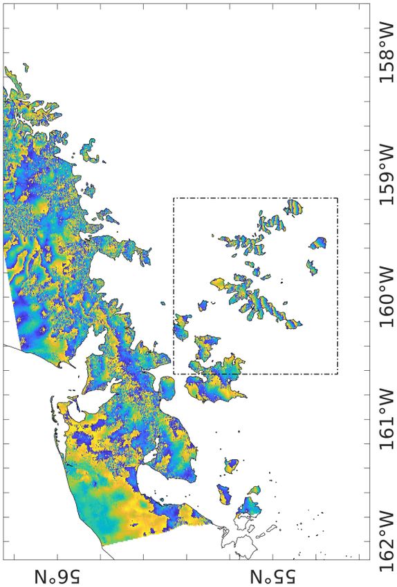
5   of 7.8, occurred at 06:12:44 UTC (22:12:44 local) on July 22 2020. On Oct
 6   19 2020 at 20:54:39 UTC (12:54:39 local), an anomalously large aftershock
 7   (M=7.6) occurred 80 km southwest of the first event. According to the U.S.
 8   Geological Survey (USGS) hypocentre catalog, both earthquakes are located
 9   on the landward side of the subduction trench. The aftershocks of the first
10   event are distributed parallel to the trench, while those of the second event
11   are aligned perpendicular to the trench. The focal mechanism solutions from
12   the Global Centroid Moment Tensor (GCMT) catalog suggest the mechanism
13   of the M7.8 event is of thrust-faulting type, while the M7.6 event was a strike-
14   slip event. The centroid depths of both earthquakes were estimated as about
15   30-35 km. This suggests that the M7.8 event ruptured the buried megathrust
16   interface, but the M7.6 event was caused by an unusual strike-slip rupture
17   along an approximately trench-normal fault.
18      The 2020 Shumagin earthquake sequence is interesting for several reasons.
19   Firstly, the mainshock is located within the Shumagin seismic gap. This
20   portion of the subduction thrust has been identified as a seismic gap since
21   the 1970s (Sykes, 1971, Davies et al., 1981). The seismic gap stretches ∼200
22   km along the Shumagin Islands and is bounded to the west by the 1946
23   Mw 8.6 earthquake (López and Okal, 2006) and to the east by the 1938 Mw 8.2
24   rupture (Freymueller et al., 2021). The last earthquakes that are inferred
25   to have ruptured through part of or the whole Shumagin gap occurred in
26   1993, 1917, 1788, and possibly 1847 (Estabrook et al., 1994). Over the last
27   century, a few moderate (M6.5 to M7.0) events have occurred in the area at
28   depths greater than 30 km. However, the fault sections ruptured by those
29   earthquakes are relatively small compared to the 200 km-long seismic gap

                                            3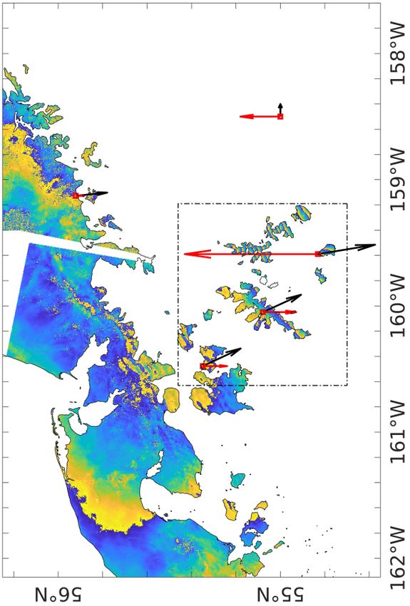
30   (e.g., the estimated rupture area of the 1993 Ms 6.9 earthquake is 40 km-long
31   and 15 km-wide, Lu et al. (1994)). If the whole Shumagin gap were fully
32   locked, the accumulated moment equates to 6.6×10¹⁹ Nm/year, assuming a
33   plate convergence rate of 64 mm/year and a uniform rigidity of 50 GPa. This
34   would require a 7.5 event every 4 years, or a M8 event every 20 years. The lack
35   of historic M7.5+ earthquakes in the Shumagin region has been explained due
36   to substantial aseismic fault creep at seismogenic depths revealed by model
37   inversions of inter-seismic GNSS velocities (Fournier and Freymueller, 2007).
38   Fournier and Freymueller (2007) suggested that instead of rupturing in large
39   earthquakes, most of the seismic moment in the Shumagin gap is released
40   through steady creep. Thus, a moderate M7 earthquake every ∼40 years, as
41   observed in the last century, may be sufficient to accommodate the residual
42   slip deficit. To the west of the Shumagin gap, a recent interseismic coupling
43   model shows that the shallow portion along the Sanak segment, 240 km-long
44   and 115 km-wide, might be partially locked, with 15%-25% coupling (Drooff
45   and Freymueller, 2021). For the shallow portion along the Sanak segment,
46   if the estimated 1946 earthquake rupture area, 180 km-long and 115 km-
47   wide (López and Okal, 2006), was fully locked, and the remaining area is
48   20% coupled, the seismic moment deficit would be accumulating at around
49   4.5×10¹⁸ Nm/year. This calculation suggests that the seismic moment of the
50   1946 earthquake, 8.5×10²¹ Nm (López and Okal, 2006), releases 1900 years
51   of elastic strain accumulation along the Sanak segment. Large uncertainties
52   are associated with estimating earthquake recurrence intervals, including the
53   poorly constrained estimation of the 1946 earthquake slip and the assumption
54   of the highest slip deficit near the trench in the interseismic coupling model

                                           4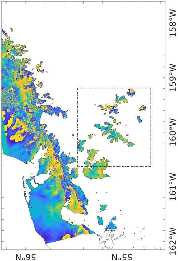
55   (Drooff and Freymueller, 2021). Nevertheless, such long recurrence intervals
56   could be the reason for there only being one documented major earthquake
57   in the Sanak segment since 1700 (Estabrook and Boyd, 1992).
58      Secondly, the M7.6 slab-breaking aftershock had an unusual strike-slip
59   mechanism and was deeply buried. Large oceanic lithosphere strike-slip
60   events have previously occurred in the oceanic plate off subduction zones,
61   such as the 2018 Mw 7.9 Gulf of Alaska earthquake (Lay et al., 2018) and
62   the 2012 Mw 8.6 Wharton basin earthquakes off-Sumatra (Wei et al., 2013).
63   In addition, the subduction zone outer-rise region regularly hosts normal-
64   faulting mechanisms events. Outer-rise normal-faulting events are attributed
65   to plate bending stresses from slab pull, and can be modulated by the in-
66   terplate seismic cycle (Ammon et al., 2008). However, the occurrence of a
67   major intraplate earthquake in the oceanic lithosphere just landward of the
68   trench is rare, with only few reported examples, such as the October 4, 1994
69   Mw 8.2 earthquake off Shikotan Island along the Kuril trench (Tanioka et al.,
70   1995). Another notable example was a Mw 7 strike-slip intraslab event lo-
71   cated beneath Kodiak Island, Alaska down-dip of the locked portion of the
72   Alaska-Aleutian megathrust (Hansen and Ratchkovski, 2001).
73      Thirdly, to our knowledge, these earthquakes are the first documented
74   sizable earthquake doublet to involve a megathrust earthquake rupture, fol-
75   lowed by an intraplate strike-slip earthquake tearing the subducting incom-
76   ing slab. Earthquake doublets are pairs of events with comparable size and
77   likely occur due to earthquake triggering interactions. Subduction earth-
78   quake doublets have been studied in the 2006-2007 Kuril and 2009 Samoa
79   doublets (Lay, 2015). In the 2006-2007 Kuril earthquake doublet, a Mw 8.4

                                          5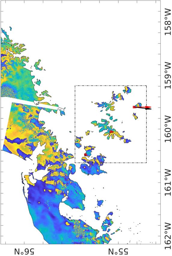
80   megathrust earthquake was followed by a Mw 8.1 earthquake rupturing an
 81   outer trench-slope normal fault, while in the 2009 Samoa earthquakes, a
 82   normal-faulting earthquake (Mw 8.1) in the outer-rise region triggered a simi-
 83   larly sized thrust-faulting earthquake (Mw 8.0) on the plate interface (Beavan
 84   et al., 2010). Therefore, detailed documentation of this doublet might con-
 85   tribute to the general understanding of the triggering mechanisms during
 86   doublets.
 87      In this paper, we use geodetic observations to determine kinematic co-
 88   seismic fault slip models of the M7.8, M7.6 earthquakes and the postseismic
 89   afterslip between two events. We investigate the major controls for the 2020
 90   Shumagin earthquake doublets. We analyze the static fault slip distribution
 91   of both events using static GNSS offsets and InSAR surface displacement
 92   measurements. The earthquakes ruptured an area off the Alaska Penin-
 93   sula covered with scattered islands, and incoherence due to water channels
 94   makes it challenging to estimate phase ambiguities during the InSAR phase
 95   unwrapping process. Hence, we take advantage of an improved Bayesian
 96   inversion of wrapped interferometric phase change observations (Jiang and
 97   González, 2020) to estimate the fault geometry and slip distribution. Our
 98   coseismic geodetic inversion results reveal that the Alaska megathrust has a
 99   complex down-dip segmentation. We propose a slab bend structure, which
100   represents a major factor controlling the occurrence and interaction during
101   this doublet, and contributes to the understanding of the mechanics of the
102   subducting oceanic lithosphere in the central Alaska subduction zone.

                                            6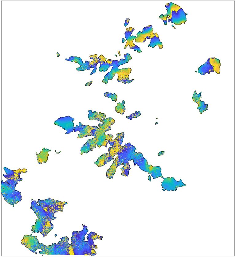
103   2. Datasets

104   2.1. GNSS dataset

105         We used three-component coseismic offsets and postseismic time series
106   from GNSS stations computed by the Nevada Geodesy Laboratory (Blewitt
107   et al., 2018). The estimated coseismic offsets of the M7.8 event were derived
108   from 5-minute sample rate time series of 108 GNSS stations, using 48 hours
109   of data before and after the mainshock. The coseismic displacements were
110   estimated by subtracting the median position after the mainshock from the
111   median position before. The coseismic displacements of the M7.6 event were
112   derived by subtracting the 24-hour final solutions of 97 GNSS station on
113   October 19 from those on October 20. For the postseismic displacements
114   between the M7.8 and M7.6 events, the displacements can be observed in
115   the GNSS time series of daily solutions. Taking station AC12 as an example,
116   the M7.8 postseismic horizontal displacements in the first day, 2 days, 24
117   days and 48 days are 0%, 4%, 19%, and 25% of the coseismic horizontal
118   displacements of the M7.8 event. Therefore, we model the 89-day postseismic
119   deformation signal between July 22 to October 19 in the following way: (1)
120   three-component daily solution of 21 GNSS stations less than 500 km away
121   from the epicenter are downloaded; (2) a parametric model is fit to the
122   time series from July 22 to October 19 with an exponential transient decay
123   function (Hearn, 2003), to obtain estimates for the displacement magnitude
124   for each station and a relaxation time (see Fig. S8); (3) we compute a
125   parametric model of postseismic GNSS displacements between July 22 and
126   October 19, and subtract the displacements on July 22 from those on October
127   19.

                                            7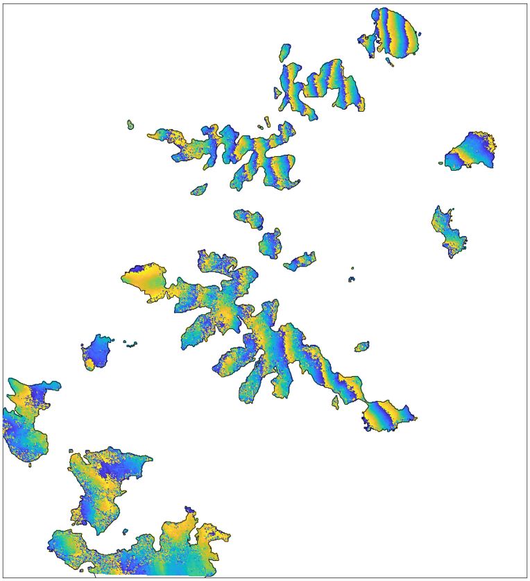
128   2.2. InSAR dataset

129      We imaged the ground surface displacement caused by the 2020 Shumagin
130   earthquake doublet using InSAR. Satellite radar interferograms capture line-
131   of-sight (LOS) motion away or towards the satellite. We used 12 European
132   Space Agency Sentinel-1 satellite interferometric wide swath mode images
133   to make six interferograms from three different satellite tracks from July 10
134   to November 7, 2020. We used data from two parallel descending tracks
135   to cover the epicentral area around the Shumagin and neighboring islands
136   (track 73 and track 102). The ascending track 153 fully images the epicentral
137   area. We processed the coseismic interferograms using the TopsApp module
138   of the ISCE software. We removed the topographic phase contribution in the
139   interferograms using SRTM 30-m resolution digital elevation model.
140      Our interferograms (Table 1) spanning the M7.8 event are dominated by
141   the coseismic deformation signals (Fig. 1(c)-(f)). We generate a preseismic
142   interferogram (Fig. S1) which is dominated by the turbulent atmosphere
143   phase delays. The two descending-track coseismic interferograms span less
144   than 2 days of early postseismic deformation. However, for the coseismic
145   interferogram in ascending track 153, the first available secondary image was
146   acquired 48 days after the earthquake. Hence it could be affected by post-
147   seismic deformation. We use the same strategy as described in Section 2.1
148   to model the 48-day postseismic deformation signal (Fig. S9), and then we
149   forward-simulate and remove the line-of-sight phase change from the ascend-
150   ing interferogram (track 152, Jul 22-Sep 08) during the first 48 days of the
151   postseismic period. Although, the correction is relatively small, our approach
152   reduces the leakage of postseismic deformation into our coseismic models.

                                            8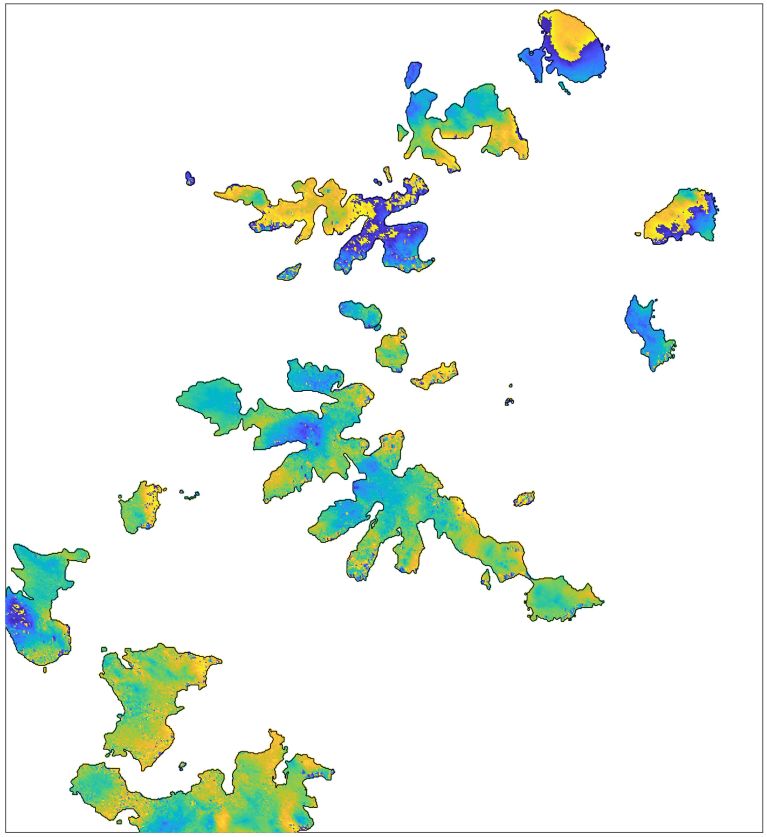
153      For the interferograms covering the M7.6 event, the interferometric phase
154   observations are also dominated by the coseismic deformation signals. The
155   estimated postseismic relaxation time for the M7.8 event is approximately
156   40 days, while the acquisition dates of the primary images of the interfero-
157   grams for the M7.6 event are 84 and 86 days after the M7.8 event, that is
158   5 and 3 days before the M7.6. Therefore, any M7.8 postseismic deforma-
159   tion signal can be considered negligible. The interferograms spanning the
160   M7.6 event might contain 7, 9 and 19 days of postseismic deformation of
161   this event. However, we did not find clear transient displacement signals ei-
162   ther in the postseismic interferograms or GNSS time series during the M7.6
163   early-postseismic period, so we performed no corrections on the coseismic
164   interferograms.

165   3. Methodology

166   3.1. Fault geometry: Non-linear surface displacement inversion

167      To determine the fault geometry of the ruptures, we invert for an elastic
168   uniform slip rectangular dislocation model. First, we solve for the fault
169   parameters using only the coseismic horizontal and vertical GNSS offsets
170   using the GBIS package (Bagnardi and Hooper, 2018). However, the sparse
171   spatial distribution of the GNSS stations does not allow to tightly constrain
172   the fault geometry (Fig. S2). Thus, we take advantage of independent high-
173   spatial-resolution InSAR observations over the Shumagin Islands and the
174   imaged far-field surface deformation over the Alaska Peninsula to refine the
175   rupture fault geometry.

                                           9
176 Standard modeling approaches of InSAR observations require unwrap-
177 ping the wrapped phase from [-π,π] to the absolute unwrapped LOS dis-
178 placements. However, phase unwrapping is an ill-posed problem requiring
179 integration along a path connecting pixels. In the Shumagin islands case,
180 the incoherence due to water channels between islands makes the phase
181 unwrapping especially challenging. Any phase unwrapping of coseismic in-
182 terferograms might contain unknown multiples of 2π between islands (see
183 Fig. S12) due to the dense gradient of fringes. Instead, our method skips
184 the phase unwrapping step, and directly inverts for fault source parameters
185 by applying the WGBIS method, a Bayesian algorithm that minimizes the
186 weighted wrapped phase residuals (Jiang and González, 2020). Now, using
187 the wrapped InSAR phase and GNSS offsets, we can constrain more tightly
188 the fault geometry parameters (Fig. 2).
189 3.2. Distributed slip models
190 Next, we propose an extension to the WGBIS method to estimate dis-
191 tributed fault slip directly from InSAR wrapped phase observations applying
192 a novel physics-based fault slip regularization. Traditional kinematic fault
193 slip inversion method used static observations to solve for the slip displace-
194 ments but neglected to consider the driving forces or stresses that cause these
195 motions. Recently, a laboratory-derived crack model was introduced to de-
196 scribe the relationship between stress and slip on the fault (Ke et al., 2020).
197 Instead of a uniform stress drop across the whole fault plane, this model
198 allows a constant stress drop in the crack center while keeping the stress
199 concentration at the rupture tip finite, and it retains a smooth transition in
200 between. The preferred shape of the crack model, an ellipse, is supported by
10201 mechanical considerations (Sendeckyj, 1970). Ke et al. (2020) proposed an
202 analytical model of the slip profile from the centre of the crack to the rup-
203 ture tip, and we expand this one-dimensional model into a two-dimensional
204 model with an elliptical shape, by assuming one of the focal points of the
205 ellipse to be the crack centre and the elliptical perimeter to be the crack tip.
206 Therefore, the slip distribution s on the fault plane is controlled by a very
207 reduced set of parameters, our crack model contains only seven parameters
208 m, s = f (m).
m = {x0 , y0 , a, e, λ, dmax , θ} (1)
209 where x0 , y0 are the locations of the focal point, and e is the eccentricity of
210 ellipse, λ is the ratio controlling the displacement transition from the center
211 to the edge of the elliptical crack, dmax is the maximum slip, and θ is the rake
212 angle. We design synthetic tests (see Fig. S13) to validate our approach, and
213 compare the performance with respect other slip-inversion methods (Amey
214 et al., 2018).
215 We name our method, the Geodetic fault-slip Inversion using a physics-
216 based Crack MOdel, hereafter referred to as GICMo. The forward model
217 proceeds as follows: (1) the crack model parameters are provided and slips
218 for all fault patches are determined based on the two-dimensional crack model
219 discussed above; (2) the surface displacements are computed by integration
220 over the fault slip distribution set; (3) for the inversion, we follow Jiang
221 and González (2020), using a misfit function based on the wrapped phase
222 residuals and the weighting matrix of observations. This misfit function is
223 then regarded as the likelihood function, and used to retrieve the posterior
224 distribution of crack model parameters by a Bayesian sampling process.
11225 We rationalize our choice for a simple elliptical crack model, firstly be-
226 cause the resolution power of InSAR and GNSS data to constrain the sub-
227 surface slip distribution decrease with the fault depth and off-shore distance.
228 Deeper earthquake sources will produce less surface deformation than shal-
229 lower events of the same size, and hence the detailed distributions of fault
230 slip of deep sources are not well resolved. Second, the published M7.8 earth-
231 quake coseismic slip distributions agree on the most notable feature: a high
232 fault slip area with rather smooth slip distribution on the plate interface
233 beneath the Shumagin Islands (Crowell and Melgar, 2020, Ye et al., 2021).
234 This first-order pattern is well resolved by our GICMo model. Third, a sim-
235 ple circular crack is also a widely accepted model to estimate the stress drop
236 of earthquakes using the observed seismic spectra (Madariaga, 1976). In
237 addition to the desirable physics-based properties (finite shear stress at the
238 crack tip), another advantage of this method is its low dimensionality. The
239 model is parametrized using fewer parameters than usually needed to de-
240 scribe the spatial pattern of slip distributions. Previous inversion algorithms
241 using deterministic or Bayesian approaches allow for highly complex patterns
242 of slip distributions by allowing unconstrained or regularized slip distribu-
243 tions (Fukahata and Wright, 2008). However, those methods are solving very
244 high dimensional problems with larger associated null-spaces, and are also
245 computationally more intensive.
246 3.3. Coulomb stress models
247 The Coulomb stress theory has been extensively applied to study the in-
248 teraction between earthquakes. Coulomb stress change induced by fault slip
249 is a quantitative measure that has been correlated with the aftershock dis-
12250 tribution, seismicity rate changes and earthquake triggering. Usually, more
251 aftershocks occur in the high stress-change region. It is thought that in-
252 creases in Coulomb stress of 0.01 MPa are sufficient to trigger events (King
253 et al., 1994). In our study, we calculate the Coulomb stress changes due to
254 the M7.8 event and investigate whether the M7.8 earthquake and its afterslip
255 promoted failure of the subsequent M7.6 event. We use the Coulomb 3.3 pro-
256 gram to carry out the stress calculations, which is based on the dislocation
257 model algorithms (https://www.usgs.gov/software/coulomb-3).
258 4. Results
259 4.1. Coseismic model for the M7.8 earthquake
260 The Shumagin earthquake nucleated near the eastern edge of the Shu-
261 magin seismic gap (Davies et al., 1981). Our static surface displacement
262 inversions suggest that the coseismic rupture extended for 112±2 km to the
263 WSW from the location of the USGS hypocentre (red rectangles in Fig. 2),
264 with an average pure thrust slip of 1.5±0.1 m, corresponding to an estimated
265 M7.8. The buried rupture extended down-dip to 44±2 km and up-dip up to
266 14±2 km depth and did not break the seafloor at the Alaska-Aleutian trench.
267 This is consistent with reports of a minor tsunami (Ye et al., 2021). A re-
268 markable feature of our inversion results is that the inferred fault geometry
269 requires a relatively steep dip angle (26±0.5 degrees, Fig. 2(b)), steeper than
270 the widely used Slab2 subduction model (∼15 degrees, Hayes et al. (2018)).
271 We further investigate this feature by separately inverting for the fault geom-
272 etry using GNSS coseismic offsets only, InSAR wrapped phase only and both
273 observations. In all cases, the obtained fault geometries are consistent with
13274 a 25-to-28 degree fault rupture plane. The GNSS only inversion suggests a
275 slightly steeper fault dip angle (Fig. S2), than the 26±0.5-degrees dip angle,
276 obtained using only the InSAR wrapped phase or both datasets (Fig. S3-S4).
277 Next, we use our estimated fault geometry model to refine the location
278 and pattern of coseismic slip during the earthquake. We tested two different
279 3D fault geometry parameterizations. The first 3D fault geometry, based
280 on the estimated fault geometry, contains two segments. A deeper segment
281 dipping 26-degree from 14 km to 44 km depth using the optimal rectangular
282 dislocation plane estimated by the non-linear inversion, and then a shallower
283 segment connecting the top edge of the rectangular plane to the trench.
284 These fault planes were then discretized into a triangular mesh with patch
285 dimensions of ∼5 km. A second geometry was obtained based on the Slab2
286 model for the Alaska megathrust, which has an average dip of 15 degrees
287 from 20 km to 50 km (Hayes et al., 2018).
288 We solve for the slip distribution of our elliptical rupture model on the
289 Slab2 and our proposed fault geometry (Fig. 2). Fig. 3 shows the observed
290 and modeled GNSS displacements and the wrapped interferometric phase,
291 as well as the residuals using the proposed down-dip structure. The modeled
292 phase is consistent with the observed phase. The root-mean-square (RMS)
293 of the GNSS residuals in the east, north and vertical directions are 0.3, 0.3
294 and 0.6 cm, and corresponding to data variance reductions of 98%, 99%,
295 and 97%. The GNSS offsets can be fit comparably well with both interface
296 geometries (see Fig. S5-S7). However, the distributed slip model on the
297 Slab2 geometry cannot reproduce the InSAR surface displacement patterns
298 as well as those with the optimized, steeper fault geometry (Fig. 3, S5-S6).
14299 Moreover, the posterior probability distribution functions on the elliptical
300 rupture model parameters are less well resolved for the Slab2 fault parame-
301 terization (Fig. S7). Our final slip model (Fig. 4(a)) shows a patch of large
302 slip near the hypocenter and below the Shumagin Islands, consistent with
303 kinematic coseismic slip models constrained using near-field high-rate GNSS
304 and strong-motion data showing a more broadly distributed slip (Crowell and
305 Melgar, 2020), and the finite-fault slip model using joint inversion of teleseis-
306 mic P and SH waves and static displacements from regional GPS stations (Ye
307 et al., 2021). The peak slip is 1.7 m, and the average slip is 0.7 m. The fault
308 slip distribution inverted from GNSS and three interferograms is shown in
309 Fig. 4(a). The total geodetic moment is 6.12×10²⁰ Nm, which is equivalent
310 to Mw 7.79, a value consistent with the seismic moment magnitude of Mw 7.8.
311 The estimated rupture centroid is located at [158.834◦ W, 55.130◦ N] and the
312 centroid focal depth is 32 km, which is deeper than the 28 km estimated by
313 USGS and 19 km away from the USGS-estimated hypocenter, [158.596◦ W,
314 55.072◦ N], in the northwest direction. Furthermore, as shown in Fig. 4(b),
315 few aftershocks are located close to the slip peak, and most seismic events
316 occurred near the edges of the estimated rupture area.
317 4.2. Postseismic model for the M7.8 earthquake
318 The M7.8 postseismic phase is important to study the whole doublet se-
319 quence, so we quantify the amount and distribution of early postseismic slip
320 caused by the M7.8 event. As afterslip is unlikely to be compact, and may
321 fully surround the coseismic rupture, the spatial distribution of postseismic
322 slip is resolved by using the slip inversion package, slipBERI (Amey et al.,
323 2018). This method incorporates the fractal properties of fault slip to regu-
15324 larize the slip distribution. We assume that afterslip dominates the observed
325 surface deformation during the 89-day-long period between the M7.8 and
326 the M7.6 events. Afterslip describes postseismic aseismic fault motions oc-
327 curring near the mainshock rupture regions over several months to several
328 years. Postseismic offsets are estimated by fitting the daily GNSS data from
329 July 22 to October 19 with a simple exponential model and then inverted
330 for the postseismic slip distribution. Compared with the coseismic model 3D
331 fault discretization, the subduction zone interface is extended along strike
332 and down-dip to investigate the distributed postseismic slip over a wider
333 area of the plate interface. The model predictions agree well with GNSS ob-
334 servations (Fig. S8), and the RMS of the GNSS residuals in the east, north
335 and vertical directions are 0.6, 0.6 and 0.7 cm, respectively.
336 We find the postseismic afterslip region mainly covered the deep portion
337 (>50km depth) of the plate interface (Fig. S10 and orange lines in Fig.
338 4(a)). A small patch, 60km-long and 40km-wide, is inferred to have slipped
339 aseismically in the very shallow portion (6-9 km depth). In the depth range
340 of 14-44 km, where the M7.8 earthquake ruptured, no strong afterslip is
341 revealed. The 3-month postseismic slip has a cumulative geodetic moment
342 of 1020 Nm, corresponding to Mw 7.27, assuming a variable crustal shear
343 modulus with depth from CRUST 1.0. We try different slip variance values
344 and rupture dimensions in slipBERI and it does not change those spatial
345 characteristics substantially.
346 Crowell and Melgar (2020) estimated the first 10 days of the postseismic
347 afterslip, finding that the majority of afterslip is concentrated downdip of
348 the mainshock between 40-60 km depth. Their model is generally consistent
16349 with our finding of afterslip dominantly occurring at greater depth. They also
350 argued that although afterslip might occur up-dip of the M7.8 earthquake,
351 the current configuration of GNSS stations is insensitive to the afterslip at
352 shallow depth. Recently, Zhao et al. (pers. comm., 2021 ) applied additional
353 constraints to regularize the afterslip distribution, where they considered
354 both stress-driven frictional models and kinematic inversions in which no
355 slip is allowed within the coseismic peak slip zone. The models of Zhao et
356 al. (pers. comm., 2021 ) suggest possible afterslip in the up-dip area of the
357 M7.8 earthquake.
358 4.3. Coseismic model for the M7.6 earthquake
359 To parameterize the geometry of the October 19 2020 M7.6 Shumagin
360 earthquake, we consider the spatial distribution of its aftershocks. Most of
361 these aftershocks occurred at the western edge of the coseismic slip area of
362 the M7.8 event. Aftershocks aligned in a north-south direction, parallel to
363 the plate convergence direction. We first approximate the dimensions of the
364 rupture area using the aftershock locations in the first two days after the
365 M7.6 event. The estimated rupture area dimensions from the aftershocks are
366 100-150 km long and 50-60 km wide and dipping 38 degrees to the east. Those
367 parameters are consistent with the focal mechanism from GCMT catalog (dip
368 angle=49◦ , strike angle=350◦ ) and the inverted parameters for a rectangular
369 dislocation source (length=50 km, width=20 km, top depth=23 km, bottom
370 depth=37 km, dip angle=44.5◦ , strike angle=358.5◦ , strike slip=3.2 m). Our
371 slip model reproduces well the coseismic deformation observed by GNSS and
372 InSAR (Fig. 3 and Fig. S11).
373 The coseismic slip model shows right-lateral strike-slip motion on a fault
17374 plane perpendicular to the Alaska subduction zone, consistent with the distri-
375 bution of the aftershocks. The aftershocks following the M7.6 event occurred
376 at the periphery of the coseismic rupture (Fig. 1(a)), effectively extending
377 the latter farther to the south and were dominated by strike-slip rupture
378 mechanisms with east-dipping north-south-striking nodal planes. The total
379 moment release from the coseismic slip was 2.1×10¹⁹ Nm, assuming a vari-
380 able crustal shear modulus with depth based on the CRUST 1.0 model. The
381 corresponding moment magnitude is Mw =7.5, in reasonable agreement with
382 the seismically determined value. We also estimated the stress drop to be 6.6
383 MPa, which is within the usual bounds of intraplate earthquakes (Allmann
384 and Shearer, 2009).
385 Our model suggests that the rupture zone is located from 23 km to 37 km
386 in depth, beneath the slab interface (Fig. 2(c)). This reveals that the M7.6
387 strike-slip earthquake ruptured the subducting oceanic slab, rather than the
388 forearc. This is also confirmed from the focal depth range of the aftershocks.
389 70% of the M2.5+ aftershocks in the first 2 days after the mainshock occurred
390 at 20-40 km depth. A significant non-double-couple component in the mo-
391 ment tensor, the substantial tsunami and the residuals of the GNSS vertical
392 component (Fig. 3(d)) indicate that another shallow rupture segment paral-
393 lel to the trench might exist (Lay, 2021), but our geodetic inversion cannot
394 resolve a second segment at shallow depth. Our inversions for two segments
395 using the geodetic data are not stable, which might be limited by the minor
396 deformation signals on the islands.
18397 5. Discussion
398 5.1. Influence of slab geometry on the rupture characteristics of the M7.8
399 earthquake
400 Our preferred coseismic rupture model constrains the deep structure of
401 the Alaska megathrust along the Shumagin segment. It reveals a ∼26 degrees
402 dipping interface from 14 to 44 km depth. The megathrust interface at
403 shallower depths is a gentler dipping segment (∼8±4 degrees) of 90 km width,
404 connecting the up-dip edge of the rupture to the trench (Fig. 2). This plate-
405 interface geometry substantially deviates from the most recent subduction
406 interface model Slab2, which is based on regionally and globally located
407 seismic events (Hayes et al., 2018). The Slab2 model suggests a 15-degrees
408 dip in the depth range from 20 to 50 km. This might indicate that the steeper
409 segment could be a relatively localized structural feature along this section
410 of the subduction zone. The discrepancy with the Slab2 model might be
411 due to smoothness constraints applied to the subduction zone model, which
412 might not resolve length-scales similar or smaller than those of the Shumagin
413 gap (100-200 km). This highlights the need to create additional regional
414 models that capture finer spatial structural details to improve subduction
415 zone seismic hazard assessment.
416 Seismic reflection imaging along profiles across the Shumagin segment
417 suggests a geometry similar to our inversion results (Li et al., 2015). In
418 Fig. 2(b), we show the interpreted seismic reflection data from Line 4 of
419 Li et al. (2015). Line 4 is located in the proximity of the M7.8 rupture
420 area, at the boundary of the Semidi segment and Shumagin seismic gap.
421 The seismic reflectors are consistent with our inferred fault geometry. Our
19422 plate interface geometry also agrees with a fault geometry grid search using
423 GNSS vertical coseismic offsets caused by the M7.8 earthquake by Crowell
424 and Melgar (2020). Their dislocation models also support a 25-degree dip
425 fault geometry, with an up-dip edge at 21±2 km and extending down to 45±5
426 km depth.
427 We also note that the M7.8 down-dip rupture limit approximately coin-
428 cides with the depth of the continental Moho, imaged by the seismic reflection
429 data at 39-41 km depth. This is consistent with a first-order correlation of
430 the base of the seismogenic zone and the base of the continental crust (e.g.,
431 Oleskevich et al. (1999)), but exceptions to this pattern have been noted
432 (Simoes et al., 2004). A zone of low-frequency tremor sources (Brown et al.,
433 2013) is located at ∼50km depth, and there is a gap between the seismo-
434 genic zone and the area hosting tremor, which is also observed in the Nankai
435 and Cascadia subduction zones (Gao and Wang, 2017). The bottom of the
436 rupture likely reached the down-dip limit of the locked seismogenic zone.
437 Recently, Shillington et al. (2021) analyzed the seismic reflection data from
438 nearby Line 5 (Fig. 2(a)) and found the continental Moho depth at 35 km,
439 with less uncertainties than Line 4 (Li et al., 2015). If this is confirmed,
440 it might suggest that part of the coseismic slip extended downdip of the
441 continental Moho (or mantle wedge corner). This coseismic slip feature was
442 previously observed in very large megathrust events, e.g. the 2010 M8.8
443 Maule, Chile, earthquake (Weiss et al., 2019). One of the explanations could
444 be that hydrated materials (e.g., serpentinites) along the base of the man-
445 tle wedge control the frictional properties of the megathrust, and allow the
446 propagation of large ruptures, even though the megathrust downdip of the
20447 mantle wedge corner is predominantly velocity strengthening (Wang et al.,
448 2020, Kohli et al., 2011).
449 Our findings suggest that the fault geometry controls the rupture size
450 and extent. A similarly large buried rupture was observed during the 2015
451 Gorkha, Nepal earthquake on a continent-continent subduction zone (Elliott
452 et al., 2016). Hubbard et al. (2016) developed a fault morphological model
453 consisting of two ramps and found that the location and shape of coseis-
454 mic fault slip (>1m) match well with the location and shape of the middle
455 decollement bounded on both sized by ramps. Therefore, they proposed that
456 the variations in fault dip angle controlled the shape and size of the main-
457 shock rupture in this continental megathrust earthquake. Decollement-ramp
458 structures formed in subducting sediments are not rare in global subducting
459 zones (Seno, 2017). About 1-km-thick subducting sediments were inferred
460 from seismic reflection data beneath the eastern Shumagin gap (Li et al.,
461 2018) and clear variations of the megathrust dipping angle were revealed at
462 7 km and 17 km (Li et al., 2015), which is consistent with the top rupture
463 depth at 14 km. In summary, the variation in fault orientation with depth
464 was likely a controlling factor limiting the extent of the Shumagin rupture.
465 5.2. The M7.6 slab-tear earthquake source region
466 If we assume that the M7.6 earthquake occurred on a pre-existing fault
467 plane, this fault had a 16-degree strike and 60-degree dip prior to being
468 subducted. This strike angle is consistent with the strike of the Kula-
469 Resurrection ridge (Fig. 6(a), Fuston and Wu (2020)). These ridges were
470 active from 60 to 40 Ma, producing north-south striking faults through the
471 seafloor spreading, and have been inactive since ∼40 Ma. The inferred dip-
21472 ping angle of the pre-existing fault is consistent with the dip angle of mid- 473 ocean-ridge normal faults. The pre-existing faults are unlikely to be formed 474 in the outer-rise region because the outer-rise bending faults are parallel to 475 the trench with approximately east-west strike directions (Shillington et al., 476 2015). The pre-existing faults are unlikely to have formed along the Pacific- 477 Kula ridge or the Pacific-Farallon ridge, because the orientation of the mag- 478 netic anomalies (east-west and northwest-southeast) are inconsistent with 479 the eventual strike of the M7.6 ruptured fault. 480 In addition, our M7.6 fault model is correlated with the location of a 481 low seismic-velocity anomaly, which has been attributed to higher slab hy- 482 dration (Li et al., 2020). Li et al. (2020) imaged the crust and uppermost 483 mantle structure of the Alaska subduction zone using ocean bottom seismo- 484 graphs and broadband seismic stations. They constructed a 3-D shear veloc- 485 ity model, where one trench-normal profile (TT1) is just
497   which might have played a major role in the location of seismogenic ruptures.
  498         Here, we propose a simple mechanical model that partially explain the
  499   location of the M7.6 event. As previously shown, the M7.6 strike-slip event
  500   ruptured the incoming slab near a bend in the down-dip geometry of the
  501   plate interface. This bend could localize deformation. Knowing that sub-
  502   ducting lithosphere is subject to flexural bending shear stresses, which are
  503   large enough to break the crust in the outer-rise region, we propose that
  504   the M7.6 could have partially been caused by accumulated flexural bending
  505   shear stresses in addition to lateral stress loading variations along the trench.
  506   Here, we assume that the rheological behaviour of the oceanic lithosphere can
  507   be approximated by that of an elastic beam. The deflection of the oceanic
  508   lithosphere is, to the first order, controlled by the gravitational body forces
  509   and bending moment acting on the descending plate (Fig. 5). So, we can
  510   compute the shear stress rate dV acting on the elastic lithosphere as a func-
  511   tion of the distance from the trench, X (Turcotte and Schubert, 2014):
  512
        √
            2π 3 eπ/4

                      Dwb         π (X − X0 )            π (X − X0 )           π (X − X0 )
dV =                          cos                + sin                   exp −                (2)
             32A (Xb − X0 )3      4 (Xb − X0 )           4 (Xb − X0 )          4 (Xb − X0 )
  513   where X0 is the location of the trench, Xb is the location deflection forebulge
  514   with height wb , and A is the slab age. The flexural rigidity parameter, D
                                            ETe3
  515   is given by the expression D =    12(1−ν 2 )
                                                     ,   which is a function of the effective
  516   elastic thickness (Te ), the Young’s modulus (E) and the Poisson’s ratio (ν).
  517   To simulate the shear stress rate dV acting on the Shumagin segment, we
  518   use parameters from Zhang et al. (2018) as listed in Table 2. The estimated
  519   shear stress rate at the location and along the length of the M7.6 rupture
  520   fault varies from 0.006 to 0.05 MPa/year. If we compare these values with

                                                23
521 respect to the coseismic stress drop, 6.6 MPa, the M7.6 event could have
522 released 130∼1100 years of accumulated bending shear stress. In addition
523 to flexural bending shear stress, shear stress directions could be controlled
524 by the slab geometry variations along trench-parallel direction. For example,
525 the downdip plate geometry from 10-50km depth along Line 5 (Shillington
526 et al., 2021) is smoother than that along Line 4 (Li et al., 2015).
527 Alternatively, shear stresses could be caused by spatial variations of elas-
528 tic coupling along the megathrust interface. Herman and Furlong (2021)
529 present models that simulate the effect of laterally variable coupling. The
530 preferred models represent the Semidi segment to be highly coupled while
531 the Shumagin segment has low coupling. The lateral displacement variations
532 can impose large-magnitude, right-lateral shear stresses on the M7.6 rupture
533 plane geometry, assuming the target fault plane was north-south striking
534 and east dipping with a dip angle 50◦ . However, we note that the available
535 geodetic observations infer only 30%±10% coupling in the western portion
536 of Semidi segment (Drooff and Freymueller, 2021) which is much lower than
537 the 100% assumed by Herman and Furlong (2021), for the whole Semidi
538 segment. Therefore, interseismic coupling variation between the Semidi and
539 Shumagin segments may contribute to the shear stress accumulation on the
540 M7.6 rupture plane, but geodetic evidence suggests this contribution may be
541 more modest in magnitude. Hence, lateral variations of coupling, the exis-
542 tence of structural weaknesses and long-accumulated bending flexural shear
543 stress could explain the occurrence of the M7.6 slab breaking event, which
544 broke the entire seismogenic thickness.
24545 5.3. Mechanisms for the interaction between the two earthquakes
546 Earthquake doublets are not uncommon and suggest short-term fault in-
547 teractions and triggering. Lay (2015) compiled 7 pairs of earthquake doublets
548 in subduction zones, where he proposed that stress transfer and triggering
549 interactions are clearly demonstrated by several doublet sequences and the
550 complexity of faulting of many of the events. To investigate the possible
551 relationship between these events, we calculate the stress perturbations on
552 the M7.6 event associated with the Jul 22 2020 M7.8 coseismic and post-
553 seismic slips (Fig. 4(d)). We utilize the inferred slip distribution from our
554 inversion model for the M7.8 event. Then, we compute the stress change on
555 the estimated fault plane of the M7.6 event. We extend the M7.6 rupture
556 fault plane along dip from the surface down to 60 km depth, and compute
557 the stress change on a regular grid with 5 km-wide patches. The M7.8 earth-
558 quake caused a shear stress increase of 0.07 MPa and tensile normal stress
559 increase of 0.27 MPa around the hypocenter, while the contributions from
560 the postseismic slip are almost neutral. Our Coulomb stress models suggest
561 that the second, M7.6 intraslab, earthquake was likely triggered by the elas-
562 tic stress changes transferred by the slip during the M7.8 coseismic slip on
563 the megathrust interface, with postseismic deformation processes possibly
564 explaining the ∼3-month delay in the occurrence of the large intraslab event.
565 6. Conclusions
566 We conclude that the 2020 Shumagin earthquake doublet represents a
567 rare example of two deeply buried ruptures on a subduction megathrust and
568 an oceanic intraplate strike-slip fault (Fig. 6(b)). The first M7.8 earth-
25569 quake partially ruptured the Shumagin seismic gap, along a 112 km-long, 65
570 km-wide section, extending from 14 km to 44 km depth. The second M7.6
571 event was likely triggered by static stress changes due to the M7.8 coseismic
572 slip and could have released 130∼1100 years of accumulated flexural bend-
573 ing shear stresses. The M7.6 broke the incoming oceanic plate at moderate
574 depths from 23 km to 37 km along a north-south striking and east-dipping,
575 right-lateral strike-slip fault. We propose that the Shumagin gap is seg-
576 mented and has variable mechanical characteristics. The M7.8 earthquake
577 ruptured a distinct eastern segment of the Shumagin gap, while the western
578 segment and shallow portions remain unruptured. We highlight that the in-
579 ferred rupture geometry of the M7.8 event is substantially steeper compared
580 to the Slab2 model. The variations of down-dip megathrust structure of the
581 Shumagin segment might have implications for seismo-tectonics and tsunami
582 hazard of this segment of the Alaska-Aleutian subduction zone, e.g., by con-
583 trolling the degree of coupling and seismic segmentation of the megathrust
584 interface (Fournier and Freymueller, 2007, Hayes et al., 2018), and influenc-
585 ing coseismic and postseismic slip distributions (Crowell and Melgar, 2020).
586 In addition, we identify Kula-Resurrection ridge fault structures imprinted
587 in the oceanic lithosphere as the likely earthquake source plane reactivated
588 during the M7.6 event. Our study highlights that the reactivation of such
589 oceanic lithospheric structures might pose an important seismic hazard in
590 subduction zones, and might represent favorable pathways for fluid flow and
591 dehydration of the subducting slab.
26592 7. Acknowledgments
593 This research was supported by the Natural Environmental Research
594 Council (NERC) through the Centre for the Observation and Modelling
595 of Earthquakes, Volcanoes and Tectonics (GA/13/M/031) and the LiCS
596 large grant (NE/K011006/1). This research was also supported by a Chi-
597 nese Scholarship Council-University of Liverpool joint scholarship awarded
598 to YJ (201706450071). PJG contribution was supported by the Spanish
599 Ministerio de Ciencia e Innovación research project, grant agreement num-
600 ber PID2019-104571RA-I00 (COMPACT) and the Beca Leonardo a Investi-
601 gadores y Creadores Culturales 2020 of the Fundación BBVA. RB acknowl-
602 edges support by NSF award EAR-1801720. Copernicus SAR data are re-
603 trieved from scihub.copernicus.eu, and 6 interferograms as well as the
604 information of 12 SAR images can be downloaded from Zenodo (https://
605 doi.org/10.5281/zenodo.xxx). The 108 and 97 GNSS stations with three-
606 component coseismic offset estimates for Jul 22 2020 M7.8 event and Oct 19
607 2020 M7.6 event are retrieved from http://geodesy.unr.edu/news_items/
608 20200723/us7000asvb_5min_rapid_20200723.txt and http://geodesy.unr.
609 edu/. The 21 GNSS stations with three-component daily offsets to estimate
610 the postseismic decay time are retrieved from Nevada Geodetic Laboratory
611 (http://geodesy.unr.edu/). The Subduction zone geometry model is re-
612 trieved from Slab2 (https://www.sciencebase.gov/catalog/item/5aa1b00ee4b0b1c392e86467/
613 The bathymetry data is retrieved from SRTM30 PLUS (https://topex.
614 ucsd.edu/WWW_html/srtm30_plus.html). The earthquake catalog is re-
615 trieved from USGS (https://earthquake.usgs.gov/earthquakes/search/).
616 The coastal data is retrieved from NOAA (https://www.ngdc.noaa.gov/
27617 mgg/shorelines/). This is a contribution of the CSIC Thematic Platform
618 PTI-Teledect (https://pti-teledetect.csic.es/). CRUST 1.0 model is
619 retrieved from https://igppweb.ucsd.edu/~gabi/crust1.html.
28Table 1: Details of Sentinel-1 interferograms for 2020 Shumagin earthquake doublet, M7.8
and M7.6 event.
Earthquake Track Direction Incidence Primary image Secondary image
date and magnitude no. (asc/des) (degree) (yyyy/mm/dd hh:mm:ss) (yyyy/mm/dd hh:mm:ss)
73 des 30-33 2020/07/10 17:03:59 2020/07/22 17:04:00
2020/07/22 06:12:44
102 des 43-46 2020/07/12 16:47:32 2020/07/24 16:47:33
M7.8
153 asc 36-41 2020/07/22 04:23:36 2020/09/08 04:23:39
73 des 30-35 2020/10/14 17:04:04 2020/10/26 17:04:04
2020/10/19 20:54:38
102 des 43-46 2020/10/16 16:47:36 2020/10/28 16:47:36
M7.6
153 asc 34-41 2020/10/14 04:23:40 2020/11/07 04:23:40
Table 2: Variables for shear stress rate calculation (Zhang et al., 2018)
Symbol Variables Value Unit
E Young’s modulus 7×10¹⁰ Pa
ν Poission’s ratio 0.25 -
Te Effective thickness of oceanic lithosphere 18.2 km
wb Height of the forebulge 0.18 km
x0 Location of the trench 0 km
xb Location where the deflection is wb 42.7 km
A Plate age 54 Ma
29168 W 164 W 160 W 156 W 152 W
50 km
(a) (b)
1964
Fig 1(c)-(f) Mw 9.2
56 N
2020/07/22 i
id
m ent
M7.8
e
54 N
1948 S gm 3000m
Se Mw 8.2
Ms 7.5 1938
m
0k
-20
km
Bathymetry
40 2020/10/19
-1
52 N
km
-80
ak M7.6
in
San ent mag
m Shu ic Gap
Seg
1946
1957 m
Mw 9.1
-20
km
Mw 8.6
Seis
-8000m
(c) (d)
2020/07/22
M7.8
AB07 Fig 3
P.
B.K.
U.
AC28 10cm
L.K.
c
N.
GPS displacement Line-of-sight Phase
AC12 S.
B. (radian)
c
C.
(e) (f)
2020/10/19
M7.6
AC12
c
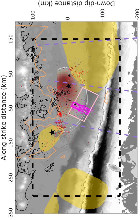
Figure 1: Tectonic background and geodetic observations of the Shumagin earthquake
doublet, 2020/07/22 M7.8 earthquake and 2020/10/19 M7.6 earthquake. (a) inset shows
the Aleutian subduction zone. Panel (b) shows historic ruptures as shaded yellow areas,
on top of the bathymetry as the background. The Shumagin seismic gap is the 200 km-
long region between the 1946 Mw 8.6 and the 1938 Mw 8.2 earthquakes. The M7.8 and
the M7.6 events are plotted as red and magenta beachballs. The first 2-day and 3-month
aftershocks following the M7.8 event are plotted as red and gray dots, where two M6+
events are plotted as little black stars. The first 2-day aftershocks following the M7.6 event
are plotted as magenta dots. The dashed box shows the boundary for images (c)-(f). Panel
(c) shows the wrapped phase of two descending interferograms, 2020/07/10-2020/07/22
(Track 73) and 2020/07/12-2020/07/24 (Track 102). The arrows show the GNSS
30Figure 1 (continued): displacements retrieved from Nevada Geodesy Laboratory, red for
vertical, and black for horizontal displacements. AB07, AC28 and AC12 are three GNSS
stations with the most significant movement. GNSS displacement at [158.5W,55N] is
the unit displacement vector for 10cm vertical and horizontal displacement. The dotted-
dashed box marks area in Fig. 3. Panel (d) shows the ascending interferogram 2020/07/22-
2020/09/08 from track 153. Panel (e) and (f) is same with Panel (c) and (d), but three
interferograms covering the M7.6 event, of two descending interferograms, 2020/10/14-
2020/10/26 (Track 73) and 2020/10/16-2020/10/28 (Track 102), and one ascending in-
terferogram, 2020/10/14-2020/11/07 (Track 153). Island abbreviations: U.: Unga; P.:
Popof; N.: Nagai; B.K.: Big Koniuji; L.K.: Little Koniuji; B.: Bird; C.: Chernabura; S.:
Simeonof.
31(a)
P’
0 km
-14
2020/07/22
km M7.8
-80
1948
Ms 7.5
Q’ 1938
Mw 8.2
2020/10/19
M7.6
-20 km
Bathymetry
1946 P
Mw 8.6 Q 64 mm/year
5 TT1 4
B.
(c) .
U.
P. N.
B. C. (b)
C. B.K.
L.K. S. Trench
S.
Trench
Lower continental
Shear velocity = 4.2 km/s crust reflection (?)
Plate interface
Continental
Moho (?) Bathymetry
Subduction depth from Slab2
Shear velocity = 4.5 km/s WGBIS-estimated fault geometry
0°
WGBIS-estimated fault geometry for 2020/07/22 M7.8 earthquake
for 2020/10/19 M7.6 earthquake 10° (dark red: optimal geometry)
(dark magenta: optimal geometry) 20° Seismic reflections
° (Line 4 in Li et al., 2015)
Upper mantle shear velocity reduction 30
(Line TT1 in Li et al., 2020) Non-volcanic tremor
Aftershock 1985 M6+ events Aftershock
Q’ Q P’ P
Figure 2: Preferred geodetic fault model constrained using InSAR wrapped phase and
GNSS. In panel (a), red and magenta rectangles outline the ensemble of inverse bayesian
fault geometry models for the M7.8 and the M7.6 earthquakes. The black line west of the
magenta rectangle indicates its projection to the surface. The dashed purple lines 4, 5 and
line TT1 indicate the position of a seismic reflection line from Li et al. (2015) and a shear
velocity profile from Li et al. (2020); the dashed gray lines are profiles PP’ and QQ’ shown
in (b) and (c). Panel (b) shows a cross-section of the inferred fault geometry models of the
M7.8 earthquake projected to profile PP’. We also show the geophysical interpretation of
the reflection lines (Line 4 and Fig. 5 in Li et al. (2015)), and locations of tremor (Brown
et al., 2013). The cross-section also shows Slab2 model (depth to the top of subducting
plate) and the bathymetry along profile PP’. Brown lines show the projected location of
islands with the same abbreviations as Fig. 1(d). Panel (c) shows a cross-section of the
inferred fault geometry models of the M7.6 earthquake projected to profile QQ’. We also
show the shear velocity reduction zone within upper mantle, constrained by the shear
32Figure 2 (continued): velocity 4.2 km/s and 4.5 km/s and digitized from Li et al. (2020). Two orange blocks present the M6+ subduct- ing events in 1985
Observation        Model    Residual
                                                             (a)
                                                                               10cm
                                                                               GPS
                                                                           displacement

                                                    Y (km)
                        GPS

                                                              50 km

                                                             (b)
                              (Descending Tracks)
         2020/07/22

                                                    Y (km)
                      InSAR
            M7.8

                                                                   10 km

                                                             (c)
                                                               .
                              (Ascending Track)
                                                    Y (km)
                      InSAR

                                                             (d)
                                                                                5cm
                                                                               GPS
                                                                           displacement
                                                    Y (km)
                        GPS

                                                              50 km

                                                             (e)
                              (Descending Tracks)
         2020/10/19

                                                    Y (km)
                      InSAR
            M7.6

                                                                   10 km

                                                             (f)
                              (Ascending Track)
                                                    Y (km)
                      InSAR

                                                                                   X (km)         X (km)    X (km)

Figure 3: The observed and modelled GNSS displacements and wrapped interferometric
phase. Images in the left column present the GNSS observations and the observed wrapped
phase for the interferograms along 2 descending tracks, as shown in the dotted-dashed box
in Fig. 1(c)-(f). Images in the middle column are the modelled GNSS and wrapped
                                                                                             34
phase based on the optimal slip distributions. Images in the right column are the residual
between observations and model.
Western Eastern
Slip (m)
segment segment
Along-strike slip Sanak Shumagin Semidi
(m) Seismic Gap Seismic Gap Segment
3 2 1 0
(c) (a) 1948
Ms 7.5
1946 1938
Mw 8.6 1
m Mw 8.2
0.
300 200 100 0
# Aftershocks 5 4 3
0
0
# Aftershocks
Down-dip slip
GPS
300 200 100
1
GPS+InSAR
(m)
(b)
2
3
0 0
(d)
10 10
M7.8 co-seismic
Depth (km)
20 20
(Jul 22)
30 30
40 40
50 50
60 60
0 0
10 10
M7.8 post-seismic
(Jul 22-Oct 19)
Depth (km)
20 20
30 30
40 40
50 50
60 60
Shear stress change (MPa) Normal stress change (MPa)
-0.05 0 0.05 -0.2 -0.1 0 0.1 0.2
Figure 4: 2020 Shumagin earthquake doublet inferred fault slip and aftershock distribu-
tion. Panel (a) presents the coseismic slip distribution estimated from GNSS offsets and
interferograms. The map is rotated so the along-strike slip is parallel to the x-axis and
along-dip slip to the y-axis. White thin lines correspond to the 0.5m slip contours for
minimum and maximum acceptable model parameters illustrating the uncertainties in the
estimated coseismic rupture models of the Jul 22 2020 M7.8 event, and white thick lines
35You can also read