Reconstructing Scenes with Mirror and Glass Surfaces - Thomas Whelan
←
→
Page content transcription
If your browser does not render page correctly, please read the page content below
Reconstructing Scenes with Mirror and Glass Surfaces
THOMAS WHELAN, Facebook Reality Labs
MICHAEL GOESELE, Facebook Reality Labs and TU Darmstadt∗
STEVEN J. LOVEGROVE, JULIAN STRAUB, and SIMON GREEN, Facebook Reality Labs
RICHARD SZELISKI, Facebook
STEVEN BUTTERFIELD, SHOBHIT VERMA, and RICHARD NEWCOMBE, Facebook Reality Labs

Fig. 1. Reconstructing a scene with mirrors. From left to right: Input color image showing the scanner with attached AprilTag in a mirror, reconstructed
geometry without taking the mirrors into account, reconstruction taking the detected mirrors (rendered as cross-hatched area) into account and a photorealistic
rendering of the scene including the mirrors. Detecting the mirrors is crucial for accurate geometry reconstruction and realistic rendering.

Planar reflective surfaces such as glass and mirrors are notoriously hard to                     1    INTRODUCTION
reconstruct for most current 3D scanning techniques. When treated naïvely,                       Active scanning techniques using Kinect-like sensors have recently
they introduce duplicate scene structures, effectively destroying the recon-
                                                                                                 been used very successfully to reconstruct indoor scenes [Kähler
struction altogether. Our key insight is that an easy to identify structure
attached to the scannerÐin our case an AprilTagÐcan yield reliable informa-
                                                                                                 et al. 2015; Newcombe et al. 2011; Nießner et al. 2013]. One fre-
tion about the existence and the geometry of glass and mirror surfaces in a                      quently occurring element of such scenesÐreflective surfaces such
scene. We introduce a fully automatic pipeline that allows us to reconstruct                     as mirrors and glassÐhas, rarely been treated in previous work.
the geometry and extent of planar glass and mirror surfaces while being able                     While this at first sounds like a minor omission, mirrors actually
to distinguish between the two. Furthermore, our system can automatically                        pose a significant problem for any reconstruction system. A perfect
segment observations of multiple reflective surfaces in a scene based on their                   mirror shows a perfect reflection of the world, which is indistin-
estimated planes and locations. In the proposed setup, minimal additional                        guishable from a direct observation of the mirrored world. The
hardware is needed to create high-quality results. We demonstrate this using                     mirror is therefore essentially łinvisiblež. The mirrored scene, how-
reconstructions of several scenes with a variety of real mirrors and glass.                      ever, will still be reconstructed using standard vision techniques.
CCS Concepts: · Computing methodologies → 3D imaging; Shape                                      Fig. 2 shows examples of bathrooms from the ScanNet dataset [Dai
modeling; Reflectance modeling;                                                                  et al. 2017] with reflected scene parts reconstructed behind mirrors.
Additional Key Words and Phrases: 3D scanning, reflective surfaces, mirrors,
                                                                                                    This mirrored geometry overlaps with real geometry located be-
glass
                                                                                                 hind the mirror and interferes with its reconstruction. It is therefore
                                                                                                 not only desirable to reconstruct mirrors as standard elements in a
ACM Reference Format:                                                                            scene, but also necessary in order to avoid invalid reconstructions
Thomas Whelan, Michael Goesele, Steven J. Lovegrove, Julian Straub, Simon                        of the overall scene. Similarly, glass surfaces are typically not recon-
Green, Richard Szeliski, Steven Butterfield, Shobhit Verma, and Richard
                                                                                                 structed by sensors but should still be included in a reconstructed
Newcombe. 2018. Reconstructing Scenes with Mirror and Glass Surfaces.
ACM Trans. Graph. 37, 4, Article 102 (August 2018), 11 pages. https://doi.org/
                                                                                                 model. Due to the prevalence of mirrors and glass in common in-
10.1145/3197517.3201319                                                                          door environments, recent scene reconstruction approaches such
                                                                                                 as Matterport3D [Chang et al. 2017] require the user to manually
*This work was carried out at Facebook Reality Labs.                                             select windows and mirrors in a scan.
Authors’ addresses: Thomas Whelan, Facebook Reality Labs, twhelan@fb.com; Michael
Goesele, Facebook Reality Labs and TU Darmstadt; Steven J. Lovegrove; Julian Straub;                In this paper, we propose a method to automatically detect and
Simon Green, Facebook Reality Labs; Richard Szeliski, Facebook; Steven Butterfield;              reconstruct mirrors and glass surfaces in a scene (see Fig. 1). Our
Shobhit Verma; Richard Newcombe, Facebook Reality Labs.                                          key idea is to add a tag to the capture rig that can only be observed
                                                                                                 when the camera faces a mirror or glass surface. In our work, we
© 2018 Copyright held by the owner/author(s). Publication rights licensed to the
Association for Computing Machinery.                                                             use a mirrored version of an AprilTag [Olson 2011; Wang and Olson
This is the author’s version of the work. It is posted here for your personal use. Not for       2016]. Based on observations of this tag, we not only detect reflective
redistribution. The definitive Version of Record was published in ACM Transactions on
Graphics, https://doi.org/10.1145/3197517.3201319.
                                                                                                 surfaces, but also robustly estimate the plane parameters of the

                                                                                             ACM Transactions on Graphics, Vol. 37, No. 4, Article 102. Publication date: August 2018.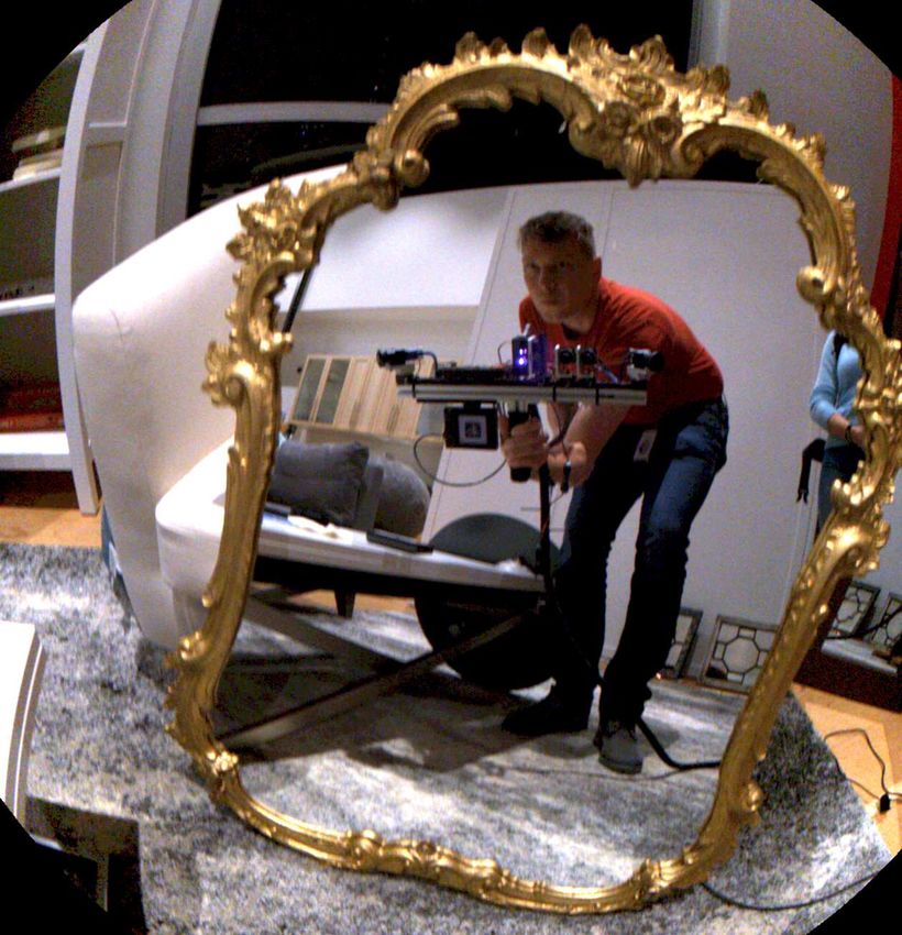
102:2 •      Whelan, Goesele, Lovegrove, Straub, Green, Szeliski, Butterfield, Verma, and Newcombe

                                                                                            approaches also rely on detecting and disentangling these two dis-
                                                                                            tinct image components. Applications include reflection removal
                                                                                            [Arvanitopoulos et al. 2017; Xue et al. 2015] and scene reconstruc-
                                                                                            tion [Sinha et al. 2012; Wang et al. 2015; Wanner and Goldluecke
                                                                                            2013]. Other approaches rely on indirect observations, such as the
                                                                                            fact that glass absorbs some light, especially in the infrared part of
                                                                                            the spectrum [Klank et al. 2011] or changes the polarization state
                                                                                            of the light [Miyazaki et al. 2004].
                                                                                               A standard mirror is covered by a thin reflecting layer at the
Fig. 2. Example scans from the ScanNet dataset [Dai et al. 2017] with                       back side of the glass. The reflection at this back side is typically
artefacts due to mirrors.                                                                   much stronger than the front reflection, leading to the well known
                                                                                            mirroring effect with hardly any observable double images. High
                                                                                            quality mirrors for scientific applications have a reflective layer
                                                                                            on the front surface (so called first surface mirrors), yielding an
surface. Additionally, we develop a multiple-feature-based approach
                                                                                            even crisper reflection. Given that we cannot observe two separate
to detect the boundary of the planar mirroring surface.
                                                                                            scenes, detecting mirror surfaces is very challenging. One option is
   Our contributions include:
                                                                                            to switch modalities, e.g., to use ultrasonic distance measurements,
     • An automatic AprilTag-based approach, where we use a mir-                            which are reflected from the mirror surface and can be reliably
       rored AprilTag to detect the existence of planar mirror or                           observed under specific imaging geometries [Yang and Wang 2008;
       glass surfaces in the scene.                                                         Zhang et al. 2017].
     • An automatic bundle adjustment-based calibration approach                               In the optical domain, there are weak signals that can be used.
       to accurately detect the plane of the reflective surface as well                     For example, time of flight scanning systems that return multiple
       as the relative tag location.                                                        observations along the line of sight may return a weak signal re-
     • An automatic approach to accurately reconstruct the bound-                           flected at the actual mirror surface. The presence of a framed mirror
       ary of framed and unframed mirror and glass surfaces and to                          can also be inferred from the observed depth discontinuity (also
       distinguish between the two surface types.                                           called a jump edge) along the mirror-frame boundary [Käshammer
     • A thorough evaluation of our approach using quantitative                             and Nüchter 2015; Yang and Wang 2011].
       measures as well as high quality renderings.                                            Active and purely passive optical approaches can detect the mirror
                                                                                            symmetry in captured images, depth images, or complete scene
2    RELATED WORK                                                                           models [Yang and Wang 2011]. While this approach can in principle
                                                                                            give a reliable indicator of the presence of a mirror in a scene, it
In this section, we survey related work on detecting and recon-                             fails if a part of the scene is only observed in the mirror and never
structing reflective surfaces and objects, focusing on the work most                        seen directly. Finally, curved specular surfaces can be detected using
relevant to our paper. We refer the reader to a recent state of the                         their distinct distortion patterns [DelPozo and Savarese 2007].
art report for more details on recovering the geometry of specular
objects [Ihrke et al. 2010]. Our work uses a prototype 3D scanner,
which implements a standard projector-camera system with an in-                             2.2 Reconstructing Reflective Surfaces
frared pattern and truncated signed distance function (TSDF) based                          The geometry of specular surfaces is typically recovered by de-
fusion. Since no modification to the scanning and reconstruction                            tecting the specular reflection of an extended target, enabling the
system is necessary, we refer the reader to the literature on KinectFu-                     estimation of a normal direction to the surface observed at a given
sion and follow-up publications for details and related work [Kähler                        pixel. The key challenge of this approach is that the target needs
et al. 2015; Newcombe et al. 2011; Nießner et al. 2013].                                    to cover all relevant angles, which would in general require it to
                                                                                            completely surround the object [Balzer et al. 2014]. Most practical
2.1 Detecting Planar Reflective Surfaces                                                    approaches therefore use a limited-size target (see, e.g., [Liu et al.
Planar glass and mirrors are difficult to detect in regular images.                         2015; Tarini et al. 2005]) that can be moved around the object and
When light hits a glass surface, most of it enters the glass, is re-                        recorded in multiple capture sessions [Balzer et al. 2011]. In the
fracted, and leaves at a different location on the back. Only a small                       limit, one can even use the specular reflection of a single point light
fraction of the light (typically less than 10%, as determined by the                        source aggregated over many frames [Chen et al. 2006]. Alterna-
Fresnel equations) is reflected on the front and back surfaces and                          tively, passive capture approaches make use of the full environment
can be observed as two distinct, faint mirror images, unless it is                          reflected in a planar [Sinha et al. 2012] or curved and more complex
masked by the scene behind the glass [Shih et al. 2015]. The fact                           surface [Godard et al. 2015]. For the special case of near-planar
that glass is a partially transparent and partially reflective surface                      surfaces, Ding and Yu [2008] interpret the reflection as observed
provides valuable information since one can actually observe two                            under orthographic projection as a general linear camera and deter-
distinct signals from the transmitted and reflected parts of the scene.                     mine its parameters from the observation of a checkerboard target.
This is widely used in multi-signal time of flight sensors [Foster et al.                   Jacquet et al. [2013] use reflections of lines in large window panes
2013; Jiang et al. 2017; Koch et al. 2017b,a]. Several passive imaging                      to reconstruct a normal field using a cut through the 3D video cube.

ACM Transactions on Graphics, Vol. 37, No. 4, Article 102. Publication date: August 2018.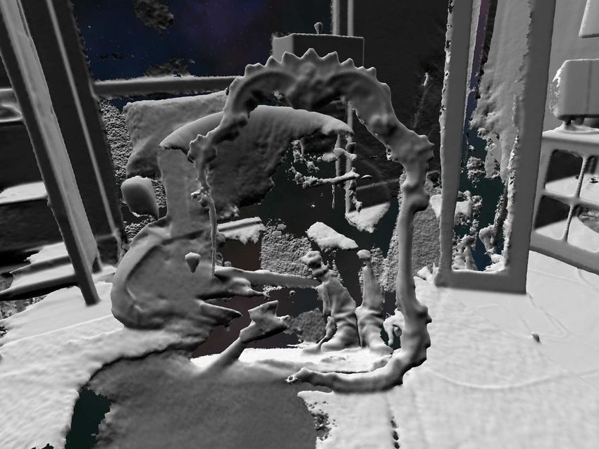
Reconstructing Scenes with Mirror and Glass Surfaces • 102:3

2.3 Scenes with Mirror and Glass Surfaces                                      area to the scanner. Since the scanner itself is typically not part of
For active scanning applications, most systems are able to scan                the scene and needs to be removed from the scan (when directly
through glass with a potential offset due to refraction. Scanning              observed or seen in a mirror), this will have no negative impact on
through a mirror surface is always possible as long as all light rays          the final scanned model.
are reflected along the same planar mirror surface. This results in               We want, however, not only to detect the fact that a mirror is
the reconstruction of a mirrored copy of the true scene geometry,              present but also to recover its position, orientation, and extent.
located behind the mirror. Fasano et al. [2003] use mirrors in order           For planar mirrors, this corresponds to finding the corresponding
to scan hard to reach areas using a laser stripe pattern scanner. Since        symmetry transform (to determine position and orientation) and
regular mirrors provided low quality scan data, the authors use first          defining the extent of the mirror plane. One way to solve the former
surface mirrors. They also propose an option for a hand-held mirror,           problem is to attach a rigid calibration target to the scanning system
whose position they detect using markers on the mirror.                        that can be detected reliably and allows the stable matching of
   Foster et al. [2013] rely on the faint diffuse reflection observed on       points on the target with feature locations in the recorded images
glass (and mirror) surfaces using a multi-return time of flight-based          [Rodrigues et al. 2010]. A simple prototype for such a system could
system. Given the physical reflection properties, glass can only be            be a standard cell phone that displays a calibration structure, records
observed in this way under a very restricted set of angles. They               images with the front-facing camera, and performs all the processing.
extend the popular occupancy grid mapping, giving it the ability to            Once calibrated, such a system could reconstruct the mirror plane
include surfaces that are only observable in a fraction of the frames          in the camera coordinate system from a single image.
in which they should have been seen.                                              In Sec. 4, we describe how we use an AprilTag-based calibration
   Jiang et al. [2017] use the intensity of the return signal for a            target attached to our scanner in order to detect glass and mirror
time-of-flight (TOF) sensor, the distance to the surface, and the              surfaces and to reconstruct the mirror plane. We currently use the
incident angle as features for a neural network-based classification           RGB camera of our scanning system for target detection, but this
of glass surfaces in indoor environments. While sufficient for robot           could also be performed in the infrared domain, where our pattern-
navigation, their approach cannot yield high accuracy scan data.               based depth camera is operating. Since our actively illuminated
   Käshammer and Nüchter [2015] detect mirrors of known geom-                  (backlit) target emits light diffusely at a luminance level similar to
etry in TOF data. They find boundaries of framed mirrors using                 the scene, it can easily be detected under a wide range of viewing
the associated jump edges in depth. A similar metric is introduced             directions while having minimal influence on scene illumination
by Yang and Wang [2011] to detect candidate mirror locations. We               or, in the infrared case, the directionally emitted high frequency
generalize the jump edge metric to also include frameless mirrors.             pattern of the projector.
Further, we use the reflection of an active tag in order to determine             Sec. 5 discusses how we jointly estimate the position of the target
mirror planes. As a result, we are able to detect planar mirrors with          with respect to the scanner and the mirror plane. We then describe
unknown, arbitrary geometry in a scene.                                        how we distinguish observations of multiple mirrors in order to
   An alternative line of work combines ultrasonic sensors with                reconstruct each of them separately (Sec. 6). In Sec. 7, we detail our
classical optical scanning in order to detect glass and mirror surfaces.       approach to accurately detect the extent of the mirror before gener-
Yang and Wang [2008] integrate a sonar sensor into a laser scanning            alizing our method to also detect glass surfaces such as windows
system to detect glass. Evidence of mirrors is detected at depth               (Sec. 8). We evaluate the full system quantitatively and qualitatively
discontinuities in the laser scans. The actual extent of a mirror              for a wide range of scenes and reflective surfaces (Sec. 9) and con-
is detected by performing an ICP based registration of real and                clude with an outlook on future work.
reflected geometry.
   Zhang et al. [2017] augment a Kinect scanning device with an                4    DETECTING A MIRROR
ultrasonic distance sensor. They look for differences in optical and           To ensure a robust detection of our target, we use AprilTags [Olson
ultrasonic depths and use an elaborate MRF-based inference in                  2011; Wang and Olson 2016], fiducial markers frequently used in the
order to detect the extent of glass and mirror surfaces. They can              robotics community. Detection using the authors’ free implementa-
also reconstruct curved surfaces by fitting a parametric surface to            tion1 happens in multiple phases. After some basic image processing
the points from the acoustic sensor. One of the key limitations of             for local intensity normalization, candidate locations are detected
ultrasonic depth sensors is that the surface needs to be observed at           as continuous bright regions containing a dark region. Next, the
near-orthogonal angles, whereas our camera has a wide field of view            edges and corners of the dark square region are extracted and the
and our tag is visible from a substantially larger set of orientations         numerical code corresponding to the tag is robustly decoded. Finally,
of the scanning rig.                                                           the edge locations are refined. Note that in order to directly use the
                                                                               existing AprilTag library, we manufactured a mirrored version of
3   OVERVIEW                                                                   the tag that can only be detected when it is observed in a mirror.
                                                                               The output of the AprilTag library is the set of detected AprilTags
The easiest way to identify a mirror or other semi-reflective surface          per frame. Each detection contains the ordered image-location of
such as glass in a scanning context is to identify the reflection of           the four corners and the tag’s center, the tag ID, as well as additional
the scanning device itself in the mirror. While this is a classical            information about the quality of the detection.
vision problem with a certain expected error rate, detection can
be simplified by adding easy to detect features such as a colorful             1 https://april.eecs.umich.edu/software/apriltag/

                                                                           ACM Transactions on Graphics, Vol. 37, No. 4, Article 102. Publication date: August 2018.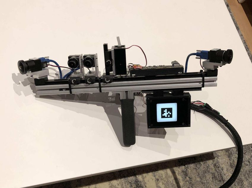
102:4 • Whelan, Goesele, Lovegrove, Straub, Green, Szeliski, Butterfield, Verma, and Newcombe
infrared RGB infrared
camera camera projector where Rba ∈ SO(3) and ab ∈ R3 is the origin of frame a expressed
in frame b such that ẋb ∝ Tba ẋa . The points xa and xb are points
in R3 ; ẋa and ẋb represents their homogeneous lifting to R4 . In our
setting, we work with three coordinate frames:
SLAM
• The corners of the AprilTag are defined in tag space t as
cameras
backlight with
ct = (± ω2 , ± ω2 , 0). ω denotes the width and height of the
AprilTag black portion of the AprilTag. The center of the AprilTag is
located at the origin of t.
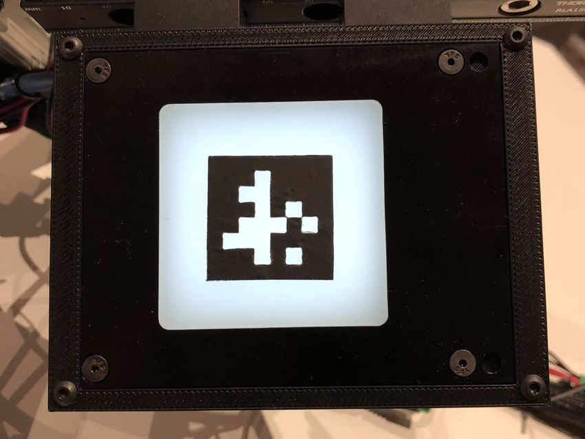
(a) Scanning rig. (b) Backlit mirrored AprilTag. • The camera defines the camera frame c with the image plane
aligned with the xy plane of the coordinate system.
Fig. 3. The prototype of the scanning rig with attached backlit AprilTag. • The world frame w is defined as the reference frame given by
the SLAM system, which also yields the per-frame transfor-
mation Tcwi from world to camera space as well as its inverse
bisection
i
Twc .
virtual virtual
camera 2 point
camera 3
V
We define the plane of the mirror N using a standard plane pa-
mirror
mirror 2 mirror 3 rameterization as " #
D
n
virtual N= ∈ R4 , (2)
tag d
virtual
camera 1 real real such that N · ẋ = 0 for points x on the plane. D
n is the unit length
tag tag
mirror 1 real real
x
normal of the plane and d is a scalar which represents the closest
camera camera
approach of the plane with the origin. Plane Na in frame a can be
expressed in frame b using the following expression: Nb = Tab ⊤ N .
a
Fig. 4. Initialization of the optimization. Left: Estimation of the mirror plane
and the tag to camera transformation from at least three virtual camera Note the unusual use of the transformation matrix Tab transposed
estimations. Right: Estimation of the mirror plane from a single frame given and not obeying the index notation ordering.
known Tc t . The symmetry transform S that transforms a point ẋa into the
virtual point v̇a as reflected in the planar mirror surface Na via
v̇a = S(Na ) ẋa is then given by
" #
The AprilTags were constructed by applying 3M 468MP pressure n) 2dD
R (D n
S (N) ≡ ∈ R4×4 (3)
sensitive adhesive to Thorlabs BKF12 black aluminum foil. The 0⊤ 1
foil was then cut on a water jet and then sandwiched between as described in Rodrigues et al. [2010]. The householder matrix
sheets of ABS plastic with the adhesive side up. (Note that this f g
supports only the manufacture of codes that consist of a single n) ≡ I3x 3 − 2D
R (D nDn⊤ ∈ R3×3 (4)
connected component.) The laminated pattern was then mounted on defines a reflection on a plane through the origin.
Metaphase backlights to ensure uniform illumination. We adjusted
the intensity of the backlights to match our overall system setup, 5.2 Generative Model
ensuring that no part of the captured tag is overexposed. Fig. 3 shows
Given the above definitions, we can now write down the reprojection
the mirrored AprilTag mounted onto the backlight and attached to j
error for pt , the j’th tag corner (or tag center) in image i, using tag
our scanning rig. The width and height of the aluminum foil tag is
coordinates t:
28.34 mm.
j i, j
i
f i, j (θ ) = πc Tcw i
S (Nw ) Twc Tct ṗt − p̃c , (5)
5 MIRROR SURFACE ESTIMATION j
where p̃c is the observed (noisy) measurement of pt in c and πc
In the following, we assume that a typical SLAM system yields an
is camera c’s projection function, R3 → R2 . We use the Kannala
accurate estimate of the pose of our scanning system for each frame
Brandt fish-eye projection model [Kannala and Brandt 2006] for
[Engel et al. 2018; Mur-Artal et al. 2015]. We formulate the problem
this function. θ is the optimization state vector consisting of the
of estimating the mirror plane as minimizing the reprojection error
tag to camera transformation Tct and the mirror plane Nw . Once
of the corner points of the AprilTag mounted to the scan head into
the system is calibrated, we can treat Tct as fixed and include only
the camera view. This requires us to define the generative model
Nw . Combining all the observations of the tag yields the following
for the projection, which we introduce in the following section.
sum-of-squares objective:
5 f
N X g2
5.1 Definitions X
F(θ ) = f i, j (θ ) , (6)
A transformation Tba of a point from coordinate frame a into a i=1 j=1
coordinate frame b is represented as
" # which we minimize using Ceres [Agarwal et al. 2018] with appro-
R ab priate initialization as described in the following section. Updates
Tba = ba ⊤ ∈ SE(3), (1)
0 1 to Tct occur on the manifold of SE(3) and we use a local minimal
ACM Transactions on Graphics, Vol. 37, No. 4, Article 102. Publication date: August 2018.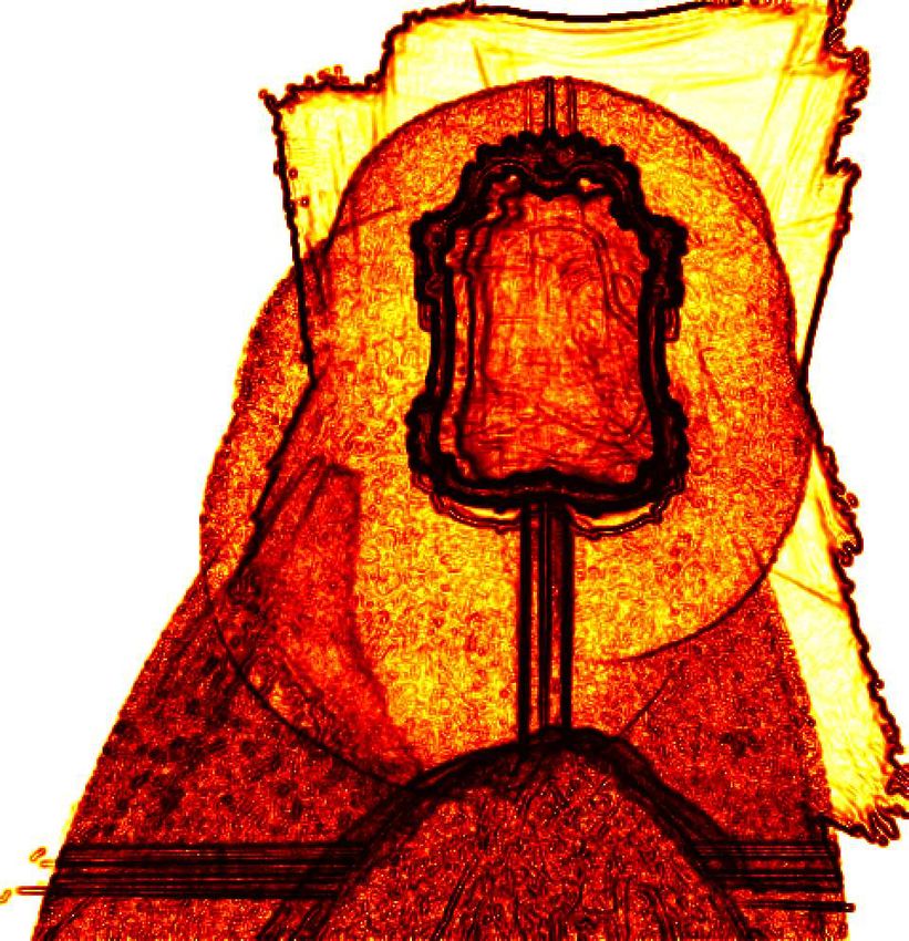
Reconstructing Scenes with Mirror and Glass Surfaces • 102:5

parameterization for optimization, ∆ct ∈ se(3) with an update step              6    MULTI-MIRROR PARAMETER ESTIMATION
at each iteration of Tct ← Tct e ∆c t . We leave the homogeneous rep-           We proceed by assuming that each AprilTag observation i belongs
resentation Nw over-parameterized and divide by the magnitude of                to its own mirror for which we can then estimate Nw    i as discussed
the first three components after convergence to reach the canonical             previously. Additionally, we can intersect the center of the 2D tag
representation as shown in Eq. 2.                                               detection with the estimated plane to find the observation point
   Although we do not do so here, our reprojection error could                  on the surface of the mirror through which our AprilTag has been
also be included as a term within a classic SLAM or structure from              reflected. Given the low false-detection rate of AprilTags, we have
motion system to improve localization and provide more thorough                 high confidence that this point belongs to a mirror surface. For each
Bayesian treatment of the complete acquisition system.                          observation, we now have a point and normal pair, [Pw    i ,D
                                                                                                                                            nwi ].
                                                                                   To separate the observations into sets for each mirror in the scene,
                                                                                we use a non-parametric clustering algorithm that we denote as
5.3 Initialization and Calibration                                              DP-planes, since it is derived from DP-means [Kulis and Jordan
Since Eq. 6, which we seek to minimize, is non-convex and Ceres                 2011] and DP-vMF-means [Straub et al. 2015]. Except for using
relies on gradient-based optimization, we must ensure an adequate               different distance metrics, these algorithms perform the same k-
initialization of the parameters to reach a globally optimal solution.          means-like alternating optimization: In step (1): incrementally assign
Rodrigues et al. [2010] describe the calibration of a system with a             data points to the closest existing cluster unless the closest cluster
fixed camera, a fixed object outside the camera’s view, and a moving            is further than some threshold λ. In the latter case, a new cluster is
planar mirror, through which the camera can observe the object.                 instantiated from the query data point. In step (2): recompute the
This is equivalent to our case of the scan system with a rigidly                cluster centers given all associated data points. For a more detailed
connected camera and tag moving in front of a static mirror.                    algorithm description, we refer to the original papers. We take the
   Following their approach, given known intrinsic calibration pa-              existing algorithm but modify the distance metric to a symmetrized
rameters for camera c and known dimensions of the AprilTag, we                  point-to-plane distance:
compute the camera from virtual-target transform Tct   i    using stan-
                                                         v                                                        1
dard exterior pose from known correspondence [Zhang 2000] for                   dist ([pa , D
                                                                                            na ], [pb , D
                                                                                                        nb ]) =                     nb ∥ + ∥ (pb − pa ) · D
                                                                                                                    (∥ (pa − pb ) · D                     na ∥) .
each image of the tag in frame i. This is depicted to the left in Fig. 4.                                         2
                                                                                                                                                            (7)
The output of the exterior pose estimation is a 6 degrees-of-freedom
transform, but the mirror plane minimally parameterized in R3 has               This distance measures how compatible two planar observations
only 3 degrees-of-freedom. The subset of SE(3) in which we ob-                  are to one another and does not require that we choose an arbitrary
serve motion informs us of the mirror plane. Given at least three               weighting between the angular and Euclidean components of the
such transforms Tct 1 , T2 , T3 , we can estimate the initial values            observations. In step (2) of the DP-planes algorithm cluster centers
                      v   ctv ctv
for the mirror plane Ñw which in turn allows us to compute the                 in the planar space are computed from the set of points pi and
                                                                                                                        Nk
real tag to camera transform T̃ct . In practice, we observed that it is         normals ni in cluster k, Ik = {pi , ni }i=1 , as
sufficient to estimate Ñw and to set T̃ct to the identity to initialize                         P                                P
                                                                                                   i ∈Ik pi                        i ∈I ni
our non-linear refinement.                                                                 pk =                         nk = P k              .  (8)
                                                                                                     Nk                          ∥ i ∈Ik ni ∥
                                                                                As in the aforementioned algorithms, the DP-planes algorithm as-
5.4 Single Image Mirror Plane Estimation                                        signs data points to cluster centers via the symmetric point-to-plane
Given the rigidity of the scanning system, we can calibrate the tag             distance if the distance is within some threshold λ, measured in
to camera transform Tct once by minimizing Eq. 6 and freezing the               meters. If the distance exceeds this threshold, a new cluster is ini-
result. This allows us to estimate the mirror plane Ñw from a single           tialized with the value of the observation. We find λ = 10 cm to
frame. Similar to above, we estimate the pose Tctv of the virtual               yield good mirror-plane segmentation in all our experiments with
(i.e., reflected) AprilTag with respect to camera c given c’s intrinsic         non-coplanar mirrors. For coplanar mirrors, we can refine the seg-
parameters and the AprilTag’s known dimension ω. The mirror                     mentation using the boundary detection (see Sec. 7) and recompute
plane can now be established as that which bisects the corresponding            the mirror plane parameters for newly segmented mirrors.
real and virtual corner locations as depicted in Fig. 4 to the right.              Equation 8 directly provides a joint estimate of the plane pa-
We use these single image mirror estimations as input for the next              rameters for each individual mirror, derived from the previously
section, where we perform a clustering step to split observations               independently estimated oriented surface samples. We use these for
from multiple mirrors and to estimate the final plane parameters                all subsequent steps.
for each mirror.
    Note that we only need to see the AprilTag in a single image and            7    MIRROR BOUNDARY DETECTION
can then transfer the observation information to all other frames
                                                                                Given the mirror plane estimated in Sec. 5, we use it as a natural
using the scene geometry and SLAM poses. Observing the mirror
                                                                                parameterization for boundary extraction. We discretize the plane
(and potentially the AprilTag) in additional frames may increase
                                                                                into a grid with square cells, typically using a resolution of 5 mm,
the accuracy of the estimated mirror plane and helps in accurately
                                                                                project all features discussed in the following onto this plane, and
detecting the mirror boundary as described in Sec. 7.
                                                                                extract the boundary using a total variation-based segmentation.

                                                                            ACM Transactions on Graphics, Vol. 37, No. 4, Article 102. Publication date: August 2018.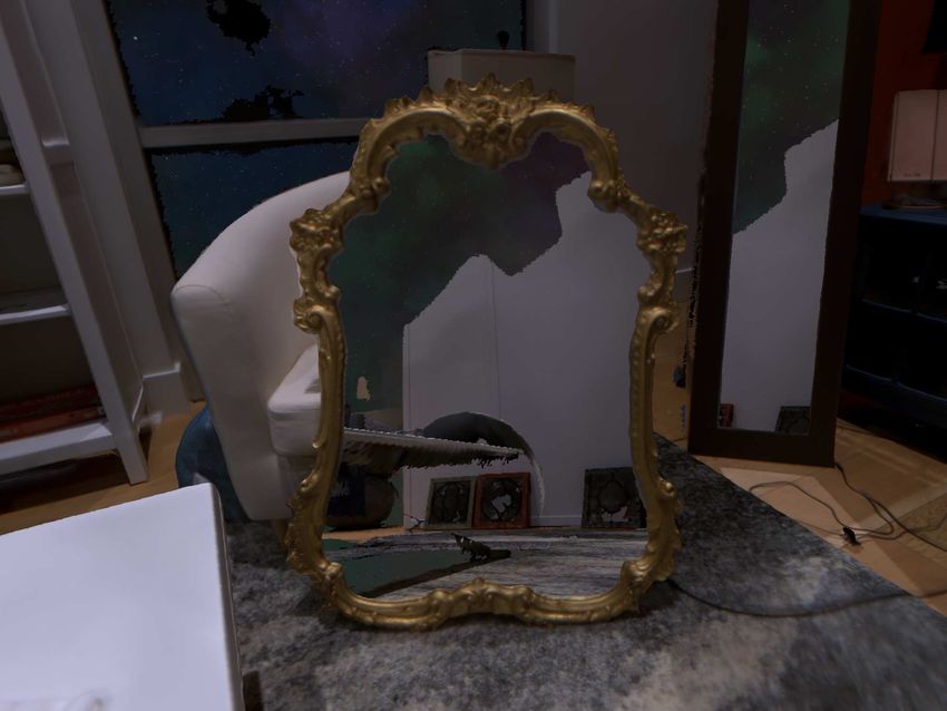
102:6 •      Whelan, Goesele, Lovegrove, Straub, Green, Szeliski, Butterfield, Verma, and Newcombe

  (a) Discontinuities     (b) Occluding         (c) Geometry          (d) Freespace           (e) σ I2         (f) ∥∇I ∥       (g) Detections     (h) ZNCC

Fig. 5. We explore eight different feature channels to facilitate mirror segmentation. All channels are shown in log-scale using the łhotž colorscheme except
the rightmost ZNCC channel which is displayed from −1 in blue to 1 in red. The first four features are computed from the depth image. The discontinuities
channel (a) indicates the mirror boundaries and Occluding (b), Geometry (c) and Freespace (b) indicate structures in front of, right around and behind the
mirror plane. Feature channels (e) and (f) aim to extract mirror boundary information from image intensities: high intensity variance σ I2 indicates a reflective
surface and high average intensity gradient ∥∇I ∥ is expected at the mirror boundary. Channel Detections (g) accumulates the AprilTag detections. Using the
zero-mean normalized cross-correlation (ZNCC) of the AprilTag appearance with the actual predicted image intensities, the ZNCC channel (h) allows us to
harvest non-mirror detections at low ZNCC-valued areas.

                                                                                            with the mirror plane and accumulate counts also for this cell. We
                                                                                            define a depth sample as belonging to a depth discontinuity if the
                                                                                            range of depth values in its 9 × 9 sample neighborhood in the depth
                                                                                            map exceeds 10 cm. We use a fairly large neighborhood since depth
                                                                                            samples right at the boundary are often not reconstructed.
         (a) д               (b) f               (c) λ               (d) u                     Intensity-based Features. To further constrain the mirror segmen-
                                                                                            tation, especially in the case of frameless mirrors, we consider two
Fig. 6. Left to right: The boundary weighting term д(x ), the segmentation                  intensity-based feature channels that use the projection of the color
constraint image f , the constraint weighting image λ, and the resulting                    images on the mirror plane: We compute the Intensity Variance
mirror segmentation image u.                                                                σI2 for each cell, i.e., the variance of the intensities projected onto
                                                                                            that cell. Because of the variability of the reflection in the mirror,
7.1 Feature Extraction                                                                      we expect high variance inside the mirror. In addition, we observe
                                                                                            higher variance for all non-reflected scene parts that are not in the
In the discretized mirror plane, we compute three sets of feature                           mirror plane. This feature is thus related to the geometric, occluding
channels. The first set is derived from geometry information, the                           and freespace features.
second set is based on image intensities, and the third set depends on
                                                                                               The Mean Intensity Gradient ∥∇I ∥ corresponds to the geo-
observations of the AprilTag. Fig. 5 visualizes the different channels
                                                                                            metric discontinuities channel. For each cell in the mirror plane, we
in log-space for a baroque-style (ornate edge) mirror (see Fig. 8j).
                                                                                            average the image gradient norm. Since two different parts of the
   Geometric Features. For the geometric features, we determine for                         scene are observed at the boundary of the mirror, this leads to a
each depth sample the intersection of the ray from the camera of the                        high average intensity gradient.
depth sensors with the mirror plane, and increment its intersection
count. We then classify each depth sample according to its signed                               Observation-based Features. The AprilTag itself yields valuable
distance d to the mirror plane as Occluding (for d > δ , i.e, for                           information. Given the properties of the AprilTag detector, we mark
samples in front of the mirror plane), Geometry close to the mirror                         for each Detection the cells covering the locations of the four cor-
plane (for −δ ≤ d ≤ δ ) or Freespace further away than the mirror                           ners and the center of the Apriltag in the mirror plane. These provide
plane (for d < −δ ). Positive distance values indicate a sample in                          strong positive evidence of a mirror.
front of the mirror plane. We use a threshold of δ = 20 mm to capture                           Finally, we compute where in an image we would see the AprilTag
depth and pose estimation noise as well as calibration inaccuracies.                        if it would be reflected in a mirror. We compute the average zero-
Each of the features is defined as the ratio of classified sample count                     mean normalized cross-correlation ZNCC [Brown 1992; Lewis 1995]
to total intersection count for each cell.                                                  between the average tag appearance and the area in the current
   One characteristic of mirrors is that they create depth discontinu-                      image at the predicted tag location assuming reflection about the
ities at their border between the reflected scene and the frame for                         mirror plane. This channel allows us in particular to harvest non-
framed mirrors [Käshammer and Nüchter 2015]. Frameless mirrors                              mirror areas as indicated by low ZNCC scores.
create a depth discontinuity between the reflected scene and the
scene behind the mirror. We capture both by determining the ratio of                        7.2 Boundary Extraction
Discontinuities in a cell, aggregated as above with one difference:                         Given the features described in the previous section, we perform
Since a discontinuity appears in a depth map as soon as a boundary                          g-weighted Total Variation segmentation [Unger et al. 2008a,b] (de-
is seen from the camera or the projector, we additionally also deter-                       tailed below), which has been used successfully in semi-supervised
mine for each sample the intersection of the projector sample ray                           image segmentation. A binary mirror/non-mirror segmentation is

ACM Transactions on Graphics, Vol. 37, No. 4, Article 102. Publication date: August 2018.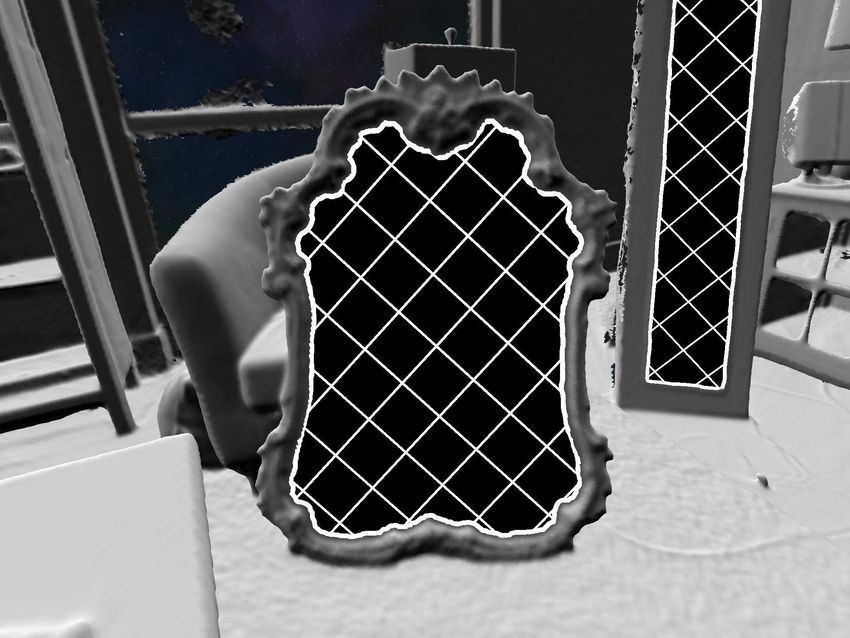
Reconstructing Scenes with Mirror and Glass Surfaces • 102:7

relaxed to real values between 0 and 1. The segmentation u is de-
fined as the solution to the following minimization over the mirror
image space Ω:
                  Z                    Z
  u ⋆ = arg min = д(x )∥∇u (x )∥d Ω+ λ(x )|u (x )− f (x )|1d Ω . (9)
         u ∈[0,1]    Ω                     Ω

д weights the boundary length regularization in the first term to en-                Fig. 7. Examples of offset observed on glass at varying distances.
courage the boundary to lead through low values in д. In the second
term, the segmentation u is constrained to be close to the function
f through the L 1 norm weighted by λ. Higher values of λ lead to a
stronger constraint on the segmentation. If λ is 0, constraints are             Any feature detection in the reflected scene must therefore be robust
not enforced.                                                                   to relatively low contrast and signal to noise ratio.
   We compute the boundary weighting term д from a combination                     Second, the reflected scene is reflected on the front and back
of the feature channels c i as                                                  surfaces of the glass, yielding a double image. This effect depends
             д(x ) = exp (− i ∈I α i ∥∇ log(c i (x ))∥γi ) ,
                             P
                                                                 (10)           on the distance of the scanning rig from the glass surface (see Ap-
                                                                                pendix A and Fig. 7). In our experience, the AprilTag library will
where we use the set of channels I = {Discontinuities, Geometry,                not detect tags if the offset is too large and will otherwise typically
Freespace, σI2 , ∥∇I ∥} and the tuned coefficients α = {0.04, 0.125,            reconstruct one of the two tag locations. It is therefore sufficient to
0.05, 0.05, 0.1} and γi = 0.8. This encapsulates the notion that we             keep a minimum distance from the glass pane while scanning.
want the mirror boundary in areas where the gradients of the feature               Third, we need to distinguish between glass and mirror surfaces.
channels are high, as can be seen from Fig. 5 and the combined д in             Our implementation classifies a surface as glass if we observe geome-
Fig. 6a.                                                                        try within the projected area of the detected AprilTag that is neither
   Using the ZNCC channel and the AprilTag detections, we set f (x )            at the depth of the AprilTag nor within δ of the reflective plane.
and λ(x ) at pixel location x to constrain the segmentation to be 1             This is only possible for glass whereas for a mirror, the AprilTag
at tag detections and 0 wherever occluding structure was detected               serves as an occluder. In other words, detection of geometry through
and at the discretized mirror plane boundaries. Additionally, we                the image of the AprilTag implies we are seeing past the surface.
incorporate weak mirror/non-mirror detections from the ZNCC                     We note that this distinction will fail for shallow objects such as
feature channel:                                                                picture frames leading to a misclassification of a glass surface as
    (1) f (x ) = 1 and λ(x ) = 103 for all target detections indicated in       mirror, shown in Fig. 15d. An alternative classification approach
        the detection feature channel,                                          would be to detect the intensity of the reflected AprilTag, which is
    (2) f (x ) = 1 and λ(x ) = 10−1 for cells with ZNCC value > 0.8,            significantly lower for glass than for a mirror.
    (3) f (x ) = 0 and λ(x ) = 10−1 for cells with ZNCC value < −0.2,              Apart from these changes, our pipeline is directly able to recon-
    (4) f (x ) = 0 and λ(x ) = 103 for the boundary of the cell domain,         struct the plane as well as the boundary of framed glass surfaces as
    (5) f (x ) = 0 and λ(x ) = 103 for cells with high Occlusion value.         we will show in the following section.
    (6) f (x ) = 0 and λ(x ) = 0 for all other pixels.
We use aggressive thresholds and a small λ value for the ZNCC-                  9    RESULTS
derived constraints to reflect the lower confidence in them, since              We implemented our reconstruction pipeline on a 6 core Intel Core
they are influenced by errors in the overall system. This ensures a             i7-5930K system with an NVIDIA TITAN Xp GPU and Ubuntu
low rate of misclassifications.                                                 16.04. The depth maps have a resolution of 960 × 640 pixels; the
   Equation 9 can be optimized efficiently and optimally as described           RGB images have a resolution of 1224 × 1024 pixels. The baseline
in Unger et al. [2008a] using a primal-dual approach yielding the seg-          reconstruction system (depth extraction, depth fusion, geometry
mentations shown in Fig. 6. We use θ = 0.1 and τ = 0.2 as proposed              extraction using dual contouring, texture generation but excluding
by Unger et al. [2008a] and iterate our GPU-based implementation                SLAM) runs on this configuration at ≈ 37 Hz. Using 12 threads, we
for 10, 000 iterations to ensure convergence.                                   can estimate the AprilTag locations in the RGB images at ≈ 70 Hz.
   We use marching squares to extract a sub-cell accurate piece-wise            The feature computation for boundary extraction runs at ≈ 38 Hz.
linear mirror boundary as the iso-contour at value 0.5 in the segmen-           The throughput of the boundary segmentation optimization is ≈
tation image u. The marching squares algorithm is the equivalent                60k pixels per second such that a 640 × 480 pixel set of feature
of marching cubes [Lorensen and Cline 1987] on a 2D grid.                       channels takes ≈ 5.12 s to segment. Overall, reconstructing a mirror
                                                                                area of ≈ 0.5 m 2 from 700 frames takes about 90 s. We used identical
8    HANDLING GLASS                                                             parameters for all results (mirrors as well as glass).
As discussed in the previous sections, glass surfaces differ from                  We demonstrate our system on a wide variety of mirrors and glass
mirrors in multiple ways. First, images of a glass surface are in               surfaces (see Fig. 8): a first surface mirror (Fig. 8a), frameless mirrors
general a mixture between the transmitted and reflected scenes.                 (Fig. 8bś8d), a beveled mirror (Fig. 8e), framed mirrors (Fig. 8fś8m),
The reflected image is therefore both diminished in brightness and              a frame mirror with texture on the mirror surface (Fig. 8h), a slightly
potentially corrupted with the texture from the direct light path.              bent mirror (Fig. 8n), and glass surfaces (Fig. 8oś8r).

                                                                            ACM Transactions on Graphics, Vol. 37, No. 4, Article 102. Publication date: August 2018.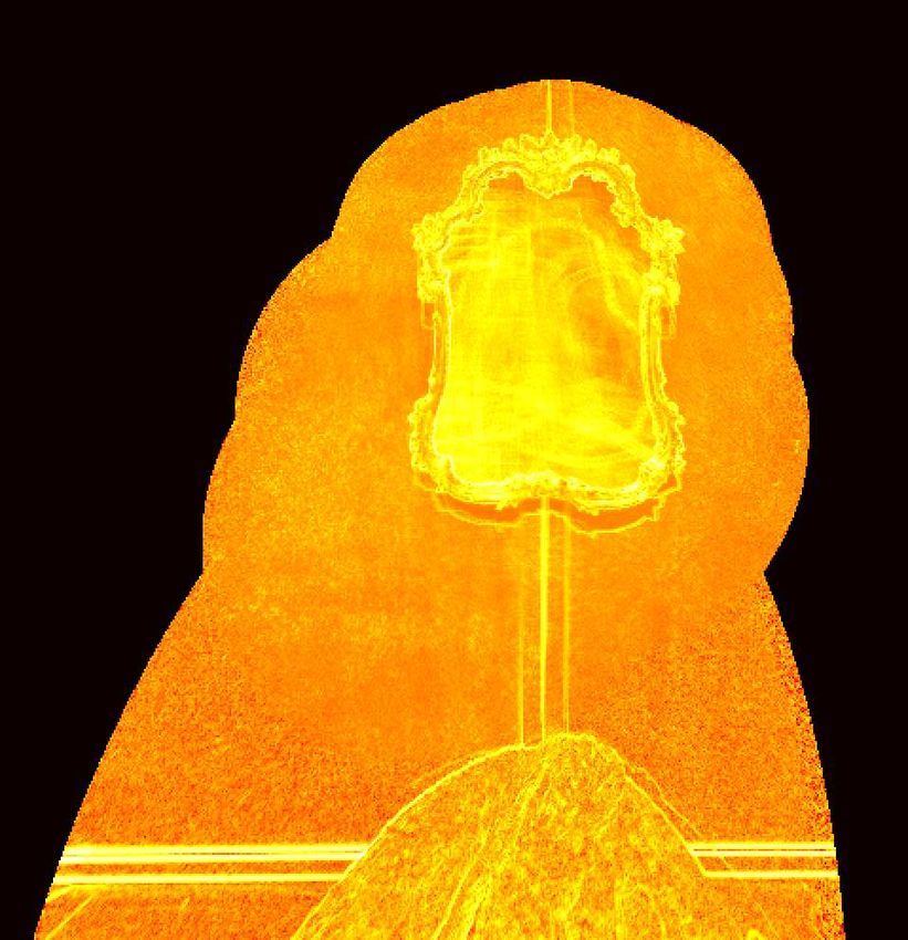
102:8 •      Whelan, Goesele, Lovegrove, Straub, Green, Szeliski, Butterfield, Verma, and Newcombe

  (a) first surface     (b) square       (c) rectangular       (d) round          (e) beveled       (f) closet   (g) door mirror   (h) textured    (i) elliptical

    (j) baroque         (k) passive     (l) double metal        (m) wall           (n) bent         (o) door     (p) blue cabinet (q) glass case    (r) kitchen

Fig. 8. Overview of the mirrors and glass surfaces used in our experiments. The first surface mirror 8a serves as ground truth flat mirror. Mirrors 8bś8e are
frameless mirrors whereas 8e is frameless with a bevel. Mirrors 8fś8m are framed. The textured mirror 8h has a printed noise texture on the mirror surface,
which is faintly visible in the image. The duplicate baroque mirror 8k is reconstructed with the illumination on the tag switched off, functioning as a passive
non-emitting tag. The double metal mirrors 8l are low quality metal-only mirrors (i.e., not based on glass). Mirror 8n is slightly bent, yielding a slimming effect.
Finally, 8oś8r show examples of glass surfaces captured.

Table 1. Error metrics (RMS error) for our reconstructions for a plane esti-                mirror plane from a single observation for all datasets. Only the
mated from a single observation (Sec. 5.4), for a plane determined by the                   door and the glass case show a noticeably larger error. The error
cluster center (Sec. 6) and for a plane estimated using the full optimization
                                                                                            of the clustering-based estimation, which jointly estimates a single
(Sec. 5.3). Reprojection errors are given in pixels; geometric errors in mm.
All values are RMS errors. The geometric error for single observations is                   plane for all observations, increases significantly as expected. The
always zero up to numerical precision. For the datasets marked with *, the                  joint full estimation based on reprojection error is able to minimize
errors are accumulated over all reflective surfaces.                                        it while typically increasing the geometric error. This is especially
                                                                                            pronounced for the wall and bent standing mirror and the datasets
  dataset             single obs.        clustering          full estimation                with multiple glass panes. We also note that the first surface mirror
                        reproj.       reproj. geom.          reproj. geom.                  yields one of the lowest geometric errors after full estimation.
                        (pixel)       (pixel) (mm)           (pixel) (mm)
  first surface          0.066          0.34     2.50          0.21     2.66
  square                 0.063          0.22     2.14          0.19     3.17                9.2 Reconstructions
  rectangular            0.056          0.36     1.77          0.34     3.51
                                                                                            In Fig. 9, we show a side by side comparison of a real world input
  round                  0.061          0.55     1.72          0.51     2.23
  beveled                0.058          1.39     2.04          1.35     8.17
                                                                                            image and the reconstruction produced by our method. Fig. 10
  closet                 0.065          0.73     2.86          0.72     6.37                shows a full scene reconstruction rendered from a novel point of
  door mirror            0.075          0.92     3.04          0.92     3.05                view. In Figs. 1 and 11 through 13, we show reconstructed surfaces
  textured               0.063          0.15     3.53          0.15     3.56                containing mirrors or glass that produce erroneous geometry when
  elliptical             0.065          0.25     2.77          0.22     3.67                not properly handling mirrors in the left column, the detected mirror
  baroque                0.059          0.54     2.11          0.50     5.64                surface and segmentation in the middle, and the rendered scene
  passive                0.066          0.92     2.76          0.56     4.67                given the reconstructed mirror on the right.
  double metal*          0.067          1.39     3.40          1.42     3.91                   For all mirror examples naïvely, fusing the depth images pro-
  wall                   0.078          3.17     1.43          2.84    16.74                duces poor reconstructions with holes where there should have
  bent                   0.075          5.61     3.54          6.33    29.46                been surfaces and erroneous reflected geometry behind the mirror
  door                    0.28          0.58     4.68          0.50     4.77                plane. While the segmentation of the frameless mirrors in Fig. 11
  blue cabinet*          0.085          1.41     2.92          1.27     5.98                is not perfect around the boundaries, it still allows us to faithfully
  glass case*            0.383          9.56      8.3          3.58     8.74                reconstruct the scene. Note that previous work is completely unable
  kitchen*               0.097          1.62     3.28          1.54     4.16                to handle such cases automatically. Our mirror segmentation can
                                                                                            handle arbitrary shaped mirror boundaries as can be seen in the
9.1 Quantitative Results                                                                    baroque-style mirror in Fig. 1. Interestingly, for the textured mirror
                                                                                            in Fig. 12, the naïve depth fusion actually partially reconstructs the
In order to quantitatively evaluate our method, we evaluate the                             mirror surfaces due to partial reflections of the IR dot pattern on the
reprojection error and the geometric error after multiple stages of                         texture. However, as can be seen, this does not disturb the proposed
our pipeline. As shown in Table 1, we can accurately estimate the

ACM Transactions on Graphics, Vol. 37, No. 4, Article 102. Publication date: August 2018.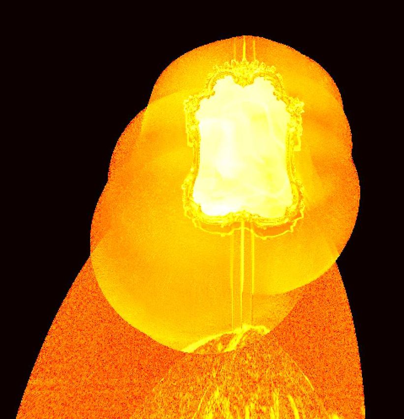
Reconstructing Scenes with Mirror and Glass Surfaces • 102:9

Fig. 9. Side by side rendering of the real world input image on the left and
our reconstruction and rendering on the right.

Fig. 10. Full scene reconstruction showing multiple reconstructed mirrors
                                                                                      Fig. 12. Top row: Framed round mirror hanging on a wall (cf. Fig. 8i). Middle
and their interreflections.
                                                                                      row: Framed mirror with some slight texture on its surface (cf. Fig. 8h).
                                                                                      Bottom row: Slightly bent free standing mirror with a frame (cf. Fig. 8n).

Fig. 11. Top row: frameless round mirror used as a table top (cf. Fig. 8d).
Bottom row: beveled mirror mounted on a wall (cf. Fig. 8e). From left to right:
Reconstructed geometry without taking mirrors into account, reconstruc-
tion taking the mirrors into account, and photorealistic rendering including
the mirrors.

                                                                                      Fig. 13. Top row: Cupboard with glass windows (cf. Fig. 8r). Bottom row:
                                                                                      Glass museum case (cf. Fig. 8q).
mirror segmentation pipeline. The slightly bent mirror in Fig. 12 is
properly approximated as a planar mirror by the proposed system.
   The glass cupboard windows in Fig. 13 are successfully recon-                        We show in Fig. 14 that our approach does not require a backlit
structed, segmented and classified as glass. Note that the pottery                    tag to achieve accurate results. In this sequence, we rely only on the
inside the cupboard is reconstructed accurately through the glass.                    ambient light available in the scene to illuminate the target. This
Although complex in nature in terms of visible reflections, our sys-                  demonstrates that our technique also works with a simple matte
tem is able to reconstruct the glass museum display case with five                    printout of an AprilTag and does not depend on difficult to source
glass panes shown in Fig. 13 without any modifications.                               custom hardware.

                                                                                  ACM Transactions on Graphics, Vol. 37, No. 4, Article 102. Publication date: August 2018.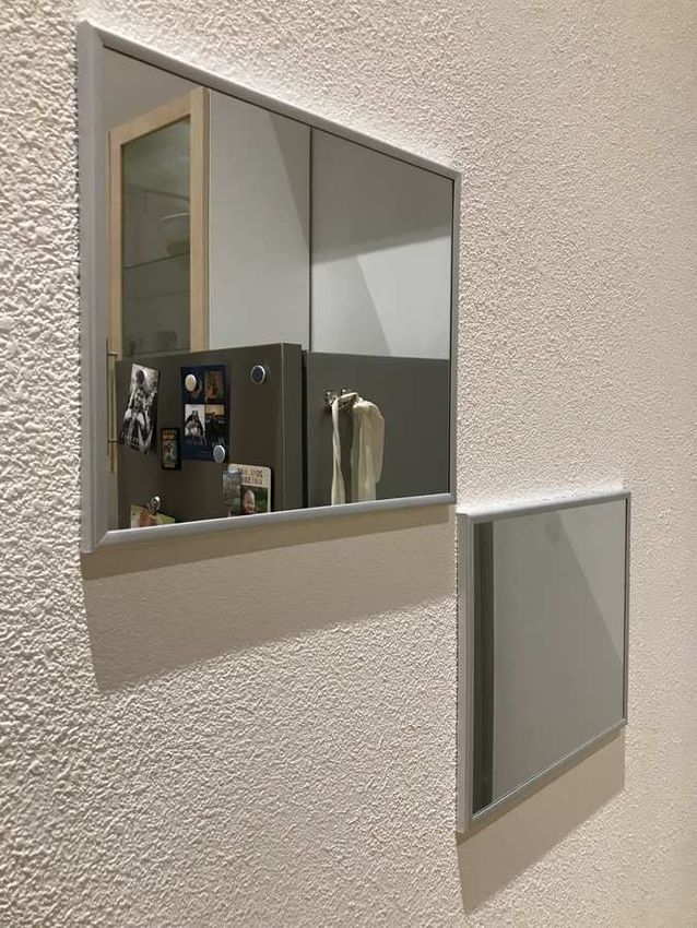
102:10 •       Whelan, Goesele, Lovegrove, Straub, Green, Szeliski, Butterfield, Verma, and Newcombe

                                                                                                                  α                α
                                                                                            thickness t
                                                                                                          glass
                                                                                                           air
                                                                                                                        θ θ

                                                                                             distance                                  offset D
                                                                                            to glass d

                                                                                                                      baseline b

                                                                                                   Fig. 16. Left: The glass configuration. Right: The offset in mm.
Fig. 14. Alternative reconstruction of the baroque mirror using a passive (i.e.,
non-illuminated) tag (see Figs. 1 and 8k). From left to right: Sample frame
from the input image sequence, reconstructed geometry, and a textured
reflecting reconstruction.

                                                                                            could be extended to account for this but would require a denser
                                                                                            set of observations to resolve the surface shape.
                                                                                               Compared to the plane estimation, detecting the boundary is
                                                                                            much more challenging since it relies on more subtle cues as can be
                                                                                            seen in many examples in this paper. In situations where the border
                                                                                            is occluded, for example in the bathroom scene in Fig. 15b, our
                                                                                            approach will not try to infer hidden structure and only resolves the
                                                                                            boundary up to the regularization capabilities of the segmentation.
                                                                                            Borderless glass presents a challenging case where the photometric
                                                                                            cues are too weak to constrain the boundary, shown in Fig. 15c.
                                                                                               As mentioned in Sec. 8, a failure case in our glass classification
                                                                                            occurs when there is geometry within δ of the estimated plane.
                                                                                            This is demonstrated in Fig. 15d with a picture frame glass that
                                                                                            is classified as mirror. As discussed previously, a remedy to this
     (a) Curved         (b) Occlusion       (c) Glass pane     (d) Picture frame
                                                                                            problem would be to calibrate the reflected intensity of the tag on
                                                                                            mirrors and glass and use that cue to distinguish between the two,
Fig. 15. Four examples of challenging structures that result in varying de-
                                                                                            as a reflection from glass would be significantly darker than one
grees of failure. The top row shows real photographs while the bottom row
shows the output of our system. These failures fall into three categories:                  from a mirror.
non-planar mirror geometry (a), lack of border observability (b, c), and
incorrect glass-mirror classification (d).                                                  10 CONCLUSION AND FUTURE WORK
                                                                                            Mirror and glass surfaces are essential components of our daily
                                                                                            environment yet notoriously hard to scan. Starting from the simple
9.3 Limitations and Failure Cases                                                           idea of robustly detecting a reflected planar target, we demonstrate
While our approach is in general highly robust, we still observed                           a complete system for robust and accurate reconstruction of scenes
occasional failure cases at various stages of the processing pipeline.                      with mirrors and glass surfaces. Given the ease of capture, our
If the AprilTag is not detected in any of the input frames, our ap-                         system could also be used to collect training data for learning-based
proach fails catastrophically. This is typically caused by bad imaging                      approaches to detect reflective surfaces. Besides our core application
conditions such as blurred images due to fast scanner movement,                             of scanning indoor scenes, we envision multiple extensions and
only partial visibility of the tag, low contrast (in particular on glass                    applications.
surfaces with both passive and back-lit targets, see also Fig. 7) or                           First, our tag requires a relatively clear reflection in order to
highly curved reflective surfaces. This could be alleviated by a more                       be detected by the AprilTag detector. Using different patterns and
visible target, e.g., a set of LEDs marking corners of a planar tag.                        detectors, one could extend our method to glossy and specular
   Given an AprilTag detection, we can always reconstruct a mir-                            surfaces. We also believe that our proposed technique could be
ror plane for a single observation using the approach described in                          extended to explicitly handle surfaces with curvature. Next, our tag
Sec. 5.4. For slightly curved mirrors, approximate reconstruction                           provides a moving, active and patterned area light. We envision that
is possible as our approach will often produce a plausible plane fit                        this could be used to also infer reflectance information about other
(e.g. Fig. 12, bottom). However, for a strongly curved mirror, our                          non-reflective surfaces in a scene. Finally, it would be interesting
representation is unable to produce an accurate estimate of the sur-                        to evaluate whether and how our approach could be integrated
face, as shown in Fig. 15a (not visible is a phantom mirror plane                           into autonomous robots, allowing them to optically detect reflective
that our approach also estimated to lie behind the surface due to                           surfaces, in particular when using only passive sensing techniques
clustering of highly distorted tag reflections). The model we use                           such as classical (multi-view) stereo.

ACM Transactions on Graphics, Vol. 37, No. 4, Article 102. Publication date: August 2018.
Reconstructing Scenes with Mirror and Glass Surfaces • 102:11
A DERIVATION OF DOUBLE IMAGES ON GLASS J. Kannala and S. S. Brandt. 2006. A generic camera model and calibration method for
conventional, wide-angle, and fish-eye lenses. PAMI 28, 8 (Aug 2006), 1335ś1340.
Fig. 16 gives the geometry for a fronto-parallel scanning rig observ- P.-F. Käshammer and A. Nüchter. 2015. Mirror identification and correction of 3D point
ing a glass pane with finite thickness. Given an incident ray hitting clouds. The International Archives of Photogrammetry, Remote Sensing and Spatial
Information Sciences 40, 5 (2015), 109.
the glass surface at an angle θ , the refracted ray inside the glass will U. Klank, D. Carton, and M. Beetz. 2011. Transparent object detection and reconstruction
travel under an angle α as determined by Snell’s law: on a mobile platform. In ICRA 2011. 5971ś5978.
Rainer Koch, Stefan May, Patrick Murmann, and Andreas Nüchter. 2017b. Identification
sin θ n glass of Transparent and Specular Reflective Material in Laser Scans to Discriminate
= (11) Affected Measurements for Faultless Robotic SLAM. Journal of Robotics and Au-
sin α n air
tonomous Systems (JRAS) 87 (2017), 296ś312.
n glass and n air are the indices of refraction of the materials. Given a R. Koch, S. May, and A. Nüchter. 2017a. Effective distinction of transparent and specular
reflective objects in point clouds of a multi-echo laser scanner. In ICAR 2017. 566ś
baseline b between the camera and the tag and a distance d between 571.
the scanning rig and the glass, the offset D(d ) can be computed as Brian Kulis and Michael I. Jordan. 2011. Revisiting k-means: New algorithms via
!! Bayesian nonparametrics. arXiv preprint arXiv:1111.0352 (2011).
n air J. P. Lewis. 1995. Fast Normalized Cross-Correlation. In Vision Interface ’95. Canadian
D (d ) = 2t tan α = 2t tan sin−1 sin θ (12) Image Processing and Pattern Recognition Society.
n glass
!!! M. Liu, R. Hartley, and M. Salzmann. 2015. Mirror Surface Reconstruction from a Single
n air b Image. PAMI 37, 4 (April 2015), 760ś773.
= 2t tan sin−1 sin tan−1 (13) William E. Lorensen and Harvey E. Cline. 1987. Marching cubes: A high resolution 3D
n glass 2d surface construction algorithm. In SIGGRAPH. ACM, 163ś169.
D. Miyazaki, M. Kagesawa, and K. Ikeuchi. 2004. Transparent surface modeling from a
Fig. 16 shows the offset D(d ) for a glass thickness of 5 mm, a relative pair of polarization images. PAMI 26, 1 (2004), 73ś82.
index of refraction nnglass
air
of 0.66 and a baseline of 0.25 m, which cor- R. Mur-Artal, J. M. M. Montiel, and J. D. Tardós. 2015. ORB-SLAM: A Versatile and
Accurate Monocular SLAM System. IEEE Transactions on Robotics 31, 5 (Oct 2015),
responds approximately to our setup. A single pixel on our AprilTag 1147ś1163.
is approximately 3.5 mm wide, which corresponds to the offset at R. A. Newcombe, S. Izadi, O. Hilliges, D. Molyneaux, D. Kim, A. J. Davison, P. Kohi, J.
Shotton, S. Hodges, and A. Fitzgibbon. 2011. KinectFusion: Real-time dense surface
roughly 0.2 m distance. mapping and tracking. In ISMAR 2011. 127ś136.
Matthias Nießner, Michael Zollhöfer, Shahram Izadi, and Marc Stamminger. 2013. Real-
REFERENCES time 3D Reconstruction at Scale Using Voxel Hashing. ACM Trans. Graph. 32, 6,
Article 169 (Nov. 2013), 11 pages.
Sameer Agarwal, Keir Mierle, and Others. 2018. Ceres Solver. http://ceres-solver.org.
Edwin Olson. 2011. AprilTag: A robust and flexible visual fiducial system. In ICRA 2011.
(2018).
3400ś3407.
N. Arvanitopoulos, R. Achanta, and S. Süsstrunk. 2017. Single Image Reflection Sup-
Rui Rodrigues, João P. Barreto, and Urbano Nunes. 2010. Camera Pose Estimation Using
pression. In CVPR 2017. 1752ś1760.
Images of Planar Mirror Reflections. In ECCV 2010. 382ś395.
J. Balzer, D. Acevedo-Feliz, S. Soatto, S. Höfer, M. Hadwiger, and J. Beyerer. 2014.
YiChang Shih, D. Krishnan, F. Durand, and W. T. Freeman. 2015. Reflection removal
Cavlectometry: Towards Holistic Reconstruction of Large Mirror Objects. In 2nd
using ghosting cues. In CVPR 2015. 3193ś3201.
International Conference on 3D Vision (3DV). 448ś455.
Sudipta N. Sinha, Johannes Kopf, Michael Goesele, Daniel Scharstein, and Richard
J. Balzer, S. Höfer, and J. Beyerer. 2011. Multiview specular stereo reconstruction of
Szeliski. 2012. Image-based Rendering for Scenes with Reflections. ACM Trans.
large mirror surfaces. In CVPR 2011. 2537ś2544.
Graph. 31, 4, Article 100 (July 2012), 10 pages.
L. G. Brown. 1992. A Survey of Image Registration Techniques. Computing Surveys 24,
Julian Straub, Trevor Campbell, Jonathan P How, and John W Fisher. 2015. Small-
4 (December 1992), 325ś376.
variance nonparametric clustering on the hypersphere. In CVPR 2015. 334ś342.
Angel Chang, Angela Dai, Thomas Funkhouser, Maciej Halber, Matthias Niessner,
Marco Tarini, Hendrik P.A. Lensch, Michael Goesele, and Hans-Peter Seidel. 2005. 3D
Manolis Savva, Shuran Song, Andy Zeng, and Yinda Zhang. 2017. Matterport3D:
acquisition of mirroring objects using striped patterns. Graphical Models 67, 4 (2005),
Learning from RGB-D Data in Indoor Environments. In 5th International Conference
233 ś 259.
on 3D Vision (3DV).
Markus Unger, Thomas Pock, and Horst Bischof. 2008a. Interactive globally optimal
Tongbo Chen, Michael Goesele, and Hans-Peter Seidel. 2006. Mesostructure from
image segmentation. Technical Report ICG-TR-08/02. Graz University of Technology.
Specularity. In CVPR 2006, Vol. 2. 1825ś1832.
Markus Unger, Thomas Pock, Werner Trobin, Daniel Cremers, and Horst Bischof. 2008b.
Angela Dai, Angel X. Chang, Manolis Savva, Maciej Halber, Thomas Funkhouser, and
TVSeg - Interactive Total Variation Based Image Segmentation. In BMVC 2008.
Matthias Nießner. 2017. ScanNet: Richly-annotated 3D Reconstructions of Indoor
J. Wang and E. Olson. 2016. AprilTag 2: Efficient and robust fiducial detection. In IROS
Scenes. In Proc. Computer Vision and Pattern Recognition (CVPR), IEEE.
2016. 4193ś4198.
A. DelPozo and S. Savarese. 2007. Detecting Specular Surfaces on Natural Images. In
Qiaosong Wang, Haiting Lin, Yi Ma, Sing Bing Kang, and Jingyi Yu. 2015. Auto-
CVPR 2007.
matic Layer Separation using Light Field Imaging. CoRR abs/1506.04721 (2015).
Yuanyuan Ding and Jingyi Yu. 2008. Recovering shape characteristics on near-flat
arXiv:1506.04721 http://arxiv.org/abs/1506.04721
specular surfaces. In CVPR 2008.
Sven Wanner and Bastian Goldluecke. 2013. Reconstructing Reflective and Transparent
J. Engel, V. Koltun, and D. Cremers. 2018. Direct Sparse Odometry. PAMI 40, 3 (2018),
Surfaces from Epipolar Plane Images. In GCPR 2013.
611ś625.
Tianfan Xue, Michael Rubinstein, Ce Liu, and William T. Freeman. 2015. A computa-
A. Fasano, M. Callieri, P. Cignoni, and R. Scopigno. 2003. Exploiting mirrors for laser
tional approach for obstruction-free photography. ACM Trans. Graph. 34, 4 (2015),
stripe 3D scanning. In 3DIM 2003. 243ś250.
79:1ś79:11.
Paul Foster, Zhenghong Sun, Jong Jin Park, and Benjamin Kuipers. 2013. VisAGGE:
Shao-Wen Yang and Chieh-Chih Wang. 2008. Dealing with laser scanner failure: Mirrors
Visible angle grid for glass environments. In CVPR 2013. 2213ś2220.
and windows. In ICRA 2008. 3009ś3015.
C. Godard, P. Hedman, W. Li, and G. J. Brostow. 2015. Multi-view Reconstruction
S. W. Yang and C. C. Wang. 2011. On Solving Mirror Reflection in LIDAR Sensing.
of Highly Specular Surfaces in Uncontrolled Environments. In 3rd International
IEEE/ASME Transactions on Mechatronics 16, 2 (April 2011), 255ś265.
Conference on 3D Vision (3DV). 19ś27.
Y. Zhang, M. Ye, D. Manocha, and R. Yang. 2017. 3D Reconstruction in the Presence of
Ivo Ihrke, Kiriakos N. Kutulakos, Hendrik P. A. Lensch, Marcus Magnor, and Wolfgang
Glass and Mirrors by Acoustic and Visual Fusion. PAMI (2017).
Heidrich. 2010. Transparent and Specular Object Reconstruction. Computer Graphics
Zhengyou Zhang. 2000. A Flexible New Technique for Camera Calibration. PAMI 22,
Forum 29, 8 (2010), 2400ś2426.
11 (Nov. 2000), 1330ś1334.
B. Jacquet, C. Häne, K. Köser, and M. Pollefeys. 2013. Real-World Normal Map Capture
for Nearly Flat Reflective Surfaces. In CVPR 2013. 713ś720.
Jun Jiang, Renato Miyagusuku, Atsushi Yamashita, and Hajime Asama. 2017. Glass
Confidence Maps Building Based on Neural Networks Using Laser Range-Finders
for Mobile Robots. In IEEE/SICE International Symposium on System Integration.
O. Kähler, V. Adrian Prisacariu, C. Yuheng Ren, X. Sun, P. Torr, and D. Murray. 2015.
Very High Frame Rate Volumetric Integration of Depth Images on Mobile Devices.
TVCG 21, 11 (Nov 2015), 1241ś1250.
ACM Transactions on Graphics, Vol. 37, No. 4, Article 102. Publication date: August 2018.You can also read