How daily groundwater table drawdown affects the diel rhythm of hyporheic exchange - HESS
←
→
Page content transcription
If your browser does not render page correctly, please read the page content below
Hydrol. Earth Syst. Sci., 25, 1905–1921, 2021
https://doi.org/10.5194/hess-25-1905-2021
© Author(s) 2021. This work is distributed under
the Creative Commons Attribution 4.0 License.

How daily groundwater table drawdown affects the
diel rhythm of hyporheic exchange
Liwen Wu1,2 , Jesus D. Gomez-Velez3,4 , Stefan Krause5,6 , Anders Wörman7 , Tanu Singh5,8 , Gunnar Nützmann1,2 , and
Jörg Lewandowski1,2
1 Department  of Ecohydrology, Leibniz-Institute of Freshwater Ecology and Inland Fisheries (IGB), Berlin, Germany
2 Geography   Department, Humboldt-University, Berlin, Germany
3 Department of Civil and Environmental Engineering, Vanderbilt University, Nashville, TN, USA
4 Department of Earth and Environmental Sciences, Vanderbilt University, Nashville, TN, USA
5 School of Geography, Earth and Environmental Sciences, University of Birmingham, Birmingham, UK
6 LEHNA-Laboratory of Ecology of Natural and Man-Impacted Hydrosystems,

University Claude Bernard Lyon 1, Lyon, France
7 Division of River Engineering, KTH-Royal Institute of Technology, Stockholm, Sweden
8 Now at Department of Numerical Mathematics, Technical University of Munich, Garching, Germany

Correspondence: Liwen Wu (liwen.wu@igb-berlin.de)

Received: 12 June 2020 – Discussion started: 6 July 2020
Revised: 10 February 2021 – Accepted: 10 February 2021 – Published: 9 April 2021

Abstract. Groundwater table dynamics extensively mod-           pollutants in the aquifer and thermal heterogeneity in the sed-
ify the volume of the hyporheic zone and the rate of hy-        iment.
porheic exchange processes. Understanding the effects of
daily groundwater table fluctuations on the tightly coupled
flow and heat transport within hyporheic zones is crucial for
                                                                Copyright statement. The works published in this journal are
water resources management. With this aim in mind, a phys-
                                                                distributed under the Creative Commons Attribution 4.0 License.
ically based model is used to explore hyporheic responses       This license does not affect the Crown copyright work, which
to varying groundwater table fluctuation scenarios. The ef-     is re-usable under the Open Government Licence (OGL). The
fects of different timing and amplitude of groundwater table    Creative Commons Attribution 4.0 License and the OGL are
daily drawdowns under gaining and losing conditions are ex-     interoperable and do not conflict with, reduce or limit each other.
plored in hyporheic zones influenced by natural flood events
and diel river temperature fluctuations. We find that both      © Crown copyright 2021
diel river temperature fluctuations and daily groundwater ta-
ble drawdowns play important roles in determining the spa-
tiotemporal variability of hyporheic exchange rates, temper-    1   Introduction
ature of exfiltrating hyporheic fluxes, mean residence times,
and hyporheic denitrification potentials. Groundwater table     Hyporheic zones are transitional areas between surface water
dynamics present substantially distinct impacts on hyporheic    and groundwater environments, which often exhibit marked
exchange under gaining or losing conditions. The timing of      physical, chemical, and biological gradients that drive the ex-
groundwater table drawdown has a direct influence on hy-        changes of water flow, energy, solute and microorganisms be-
porheic exchange rates and hyporheic buffering capacity on      tween surface and subsurface regions (Boano et al., 2014).
thermal disturbances. Consequently, the selection of aquifer    Although the hyporheic zone is a small veneer, it has dis-
pumping regimes has significant impacts on the dispersal of     proportionately significant effects on nutrient cycling and
                                                                river ecological functioning (Malcolm et al., 2002; Krause
                                                                et al., 2009; Gomez-Velez et al., 2015). Understanding the

Published by Copernicus Publications on behalf of the European Geosciences Union.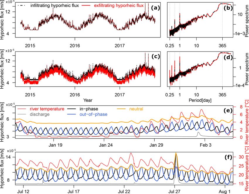
1906                 L. Wu et al.: How daily groundwater table drawdown affects the diel rhythm of hyporheic exchange

spatiotemporal variability of hyporheic exchange processes             Groundwater table fluctuations are observed across mul-
is key to characterizing the nutrient cycling and river ecosys-     tiple temporal scales. On seasonal scales, rainfall and
tem functioning (Lewandowski et al., 2019).                         irrigation pumping following well-defined seasonal cy-
   Hydrological drivers and modulators of time-varying hy-          cles cause groundwater table fluctuations; on daily scales,
porheic exchange processes have been extensively stud-              phreatophyte-induced water use (long-rooted plants take up
ied in the last decade. The hydraulic gradient as the main          water from the saturated zone) and anthropogenic pump-
driver of hyporheic exchange processes is changing along the        ing activities are the main causes for groundwater table
sediment–water interface, determining (1) the spatiotempo-          fluctuations; on event scales, groundwater tables fluctuate
ral variability of hyporheic zone extents and (2) character-        in response to storm events (Todd and Mays, 2005; Butler
istic timescales of hyporheic exchange (Boano et al., 2013;         et al., 2007; Malzone et al., 2016). Both numerical model-
Ward et al., 2017; Gomez-Velez et al., 2017). Factors influ-        ing studies and field observations indicate that groundwater
encing the hydraulic gradient at the sediment–water inter-          table fluctuations have significant control on the hydraulic
face include channel flow (Trauth and Fleckenstein, 2017;           gradient change at the sediment–water interfaces, which is
Grant et al., 2018; Broecker et al., 2018; Singh et al., 2020),     the main driver of transient hyporheic responses (Malcolm
geomorphological settings (Tonina and Buffington, 2011;             et al., 2006; Voltz et al., 2013; Malzone et al., 2016). How-
Schmadel et al., 2016; Singh et al., 2019; Chow et al., 2019),      ever, these studies are usually focused on seasonal- and
and regional groundwater flow (Nützmann et al., 2014; Mal-          event-scale groundwater table fluctuations. The role of daily
zone et al., 2016; Wu et al., 2018). Sediment and fluid             groundwater table fluctuations for hyporheic exchange pro-
properties do not drive hyporheic exchange, but they modu-          cesses requires more attention.
late hyporheic exchange substantially: sediment heterogene-            River temperature often fluctuates with a clear daily cycle
ity can alter hyporheic flow paths and residence time dis-          in response to the diurnal change in solar radiation (Caissie,
tributions, creating hot spots for biogeochemical transfor-         2006). This daily change in river temperature directly af-
mations (Sawyer and Cardenas, 2009; Gomez-Velez et al.,             fects water viscosity and density, and subsequently the hy-
2014; Pescimoro et al., 2019; Chow et al., 2020; Earon et al.,      draulic conductivity of the sediment. As a consequence, hy-
2020); fluid properties, i.e., density and viscosity, are func-     porheic exchange rates often exhibit a diel fluctuation pat-
tions of temperature and directly influence the hydraulic con-      tern due to the temperature-dependent hydraulic conductiv-
ductivity, thus hyporheic flow. Consequently, river tempera-        ity that governs the flow transport in the sediment. Wu et al.
ture variability (i.e., diel and seasonal river temperature fluc-   (2020) observed that hyporheic exchange fluxes inherit the
tuations) induces significant changes of hyporheic exchange         daily-scale spectral signatures from river temperature fluctu-
processes (Cardenas and Wilson, 2007a). The spatiotem-              ations and noticeably, however, these signatures are absent
poral variability of the drivers and modulators eventually          in river discharge of the studied site. This observation evi-
results in dynamic hyporheic exchange processes. Among              dently indicates a strong control of the diel river temperature
these drivers and modulators, the combined effects of re-           fluctuations on hyporheic exchange processes. However, the
gional groundwater flow and river temperature on dynamic            temperature-dependent diel rhythm of hyporheic exchange
hyporheic exchanges are comparably understudied.                    rates can be influenced by the daily groundwater table fluctu-
   Depending on the direction of net groundwater flow, the          ations due to evapotranspiration and anthropogenic pumping
river can be gaining when groundwater discharges into the           activities. Therefore, understanding the two players, namely
river, or losing when river recharges the aquifer (Winter et al.,   daily groundwater hydraulic gradient change (as a result of
1998) (Fig. 1a). Different directions of groundwater flow           daily groundwater table fluctuations) and diel hydraulic con-
result in substantially different flow fields (Fig. 1b and c).      ductivity change (as a result of diel river temperature fluctu-
Large groundwater upwelling and downwelling may com-                ations), is important to characterize dynamic hyporheic ex-
press the hyporheic zone’s spatial extent and reduce the hy-        change processes.
porheic exchange flow rate. Nevertheless, most of the previ-           In the present study, we aim to quantify the impact of river
ous numerical modeling studies about the impact of ground-          temperature fluctuations and groundwater table drawdown
water direction on hyporheic exchanges are either limited to        on hyporheic exchange processes at daily scales, as well as
steady hydrological conditions and/or uniform groundwater           to better understand implications on the hyporheic zone’s po-
flow conditions (Cardenas and Wilson, 2006, 2007b; Boano            tential for denitrification and thermal buffering. With these
et al., 2008; Trauth et al., 2013; Marzadri et al., 2016; Wu        objectives in mind, a series of synthetic groundwater scenar-
et al., 2018). Although there are recent field investigations       ios corresponding to different timings of groundwater table
on the role of transient groundwater table fluctuations in          drawdown under gaining and losing conditions is applied in
hyporheic exchange processes (Malcolm et al., 2006; Ward            a physically based hyporheic flow and heat transport model.
et al., 2013; Zimmer and Lautz, 2014), they usually lack a          Hyporheic exchange rates, temperature distribution, and den-
quantification of the impact of groundwater table dynamics          itrification efficiency are quantified to assess the impacts of
on hyporheic exchange processes (Malzone et al., 2016).             river temperature and groundwater level fluctuations on hy-
                                                                    porheic exchange processes. Our findings provide insights

Hydrol. Earth Syst. Sci., 25, 1905–1921, 2021                                        https://doi.org/10.5194/hess-25-1905-2021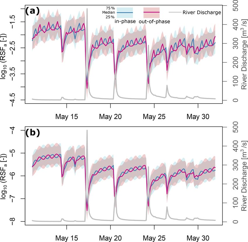
L. Wu et al.: How daily groundwater table drawdown affects the diel rhythm of hyporheic exchange                                    1907

Figure 1. Schematic description of (a) gaining and losing groundwater systems and bedform-induced hyporheic exchanges under (b) gaining
and (c) losing conditions. The river can be gaining when groundwater discharges into the river (scenario of groundwater table A) or losing
when the river recharges the aquifer (scenario of groundwater table B). Different directions of groundwater flow result in substantially
different flow field, location, and geometry of hyporheic zones.

into the dynamic hyporheic responses to impacts of daily               2.2     Model for coupled flow and heat transport
groundwater withdrawal and river temperature fluctuations
for the first time, allowing for a better mechanistic under-           2.2.1    Model for groundwater flow
standing of hyporheic exchange processes and hence an im-
proved pumping operational scheme.                                     Groundwater flow is described using Darcy’s law in a non-
                                                                       deformable porous medium (Bear, 1972). The top bound-
                                                                       ary is a Dirichlet boundary. Lateral boundaries are periodic
2     Methods                                                          boundaries, representing an infinite domain in the longitudi-
                                                                       nal direction. The bottom boundary is either prescribed in-
2.1    Model domain                                                    flow for groundwater gaining conditions (qb (+)) or outflow
                                                                       for groundwater losing conditions (qb (−)):
To understand the hyporheic exchange in response to chang-
ing river discharge, temperature, and groundwater table fluc-

                                                                         ∂ρ           κ
tuations, a two-dimensional conceptualization is proposed              θ    = ∇ · ρ (∇p + ρg∇h)                                 (1a)
                                                                         ∂t           µ
based on Wu et al. (2018) and Wu et al. (2020) (Fig. 2a).
                                                                       p(x, y = Zbed (x), t) = ρg hSWI (x, t) for ∂SWI         (1b)
The sediment is assumed homogeneous and isotropic with a
sinusoidal sediment–water interface of wavelength λ and am-            p(x = −λ, y, t) = p(x = 2λ, y, t) + ρg[hSWI (x = −λ, t)
plitude 1, representing periodic bedforms. The streamwise                   + hSWI (x = 2λ, t)] for ∂u and ∂d                      (1c)
length (L) is 3λ and the depth of the model domain (dgw ) is
                                                                             κ

5λ, respectively. Bedforms are assumed stationary and fully            n · − (∇p + ρg∇z) = −qb for ∂b ,                             (1d)
                                                                             µ
saturated. Transport of flow, solute, and heat is simulated by
using COMSOL Multiphysics (version: 5.4) with the finite               where t is time [T], θ is porosity [–] as 0.3, p(x, t) is pressure
element method using a mesh with telescopic refinement near            [ML−1 T−2 ], g is gravitational acceleration [LT−2 ], κ is per-
the boundaries and approximately 54 000 elements. The sim-             meability [L2 ] as 1 × 10⁻¹⁰ m2 , ρ is fluid density [ML−3 ], µ
ulations are mesh independent. The computation time for a              is fluid dynamic viscosity [ML−1 T−1 ], Darcy velocity is q =
full-length scenario is around 60 h.                                   − µκ (∇p + ρg∇h)) [LT−1 ], Zbed (x) = (1/2) sin(2π x/λ) is
                                                                       the elevation of the water–sediment interface [L], n is an out-
                                                                       ward vector normal to the boundary [–], and qb is groundwa-
                                                                       ter flux [LT−1 ].

https://doi.org/10.5194/hess-25-1905-2021                                            Hydrol. Earth Syst. Sci., 25, 1905–1921, 2021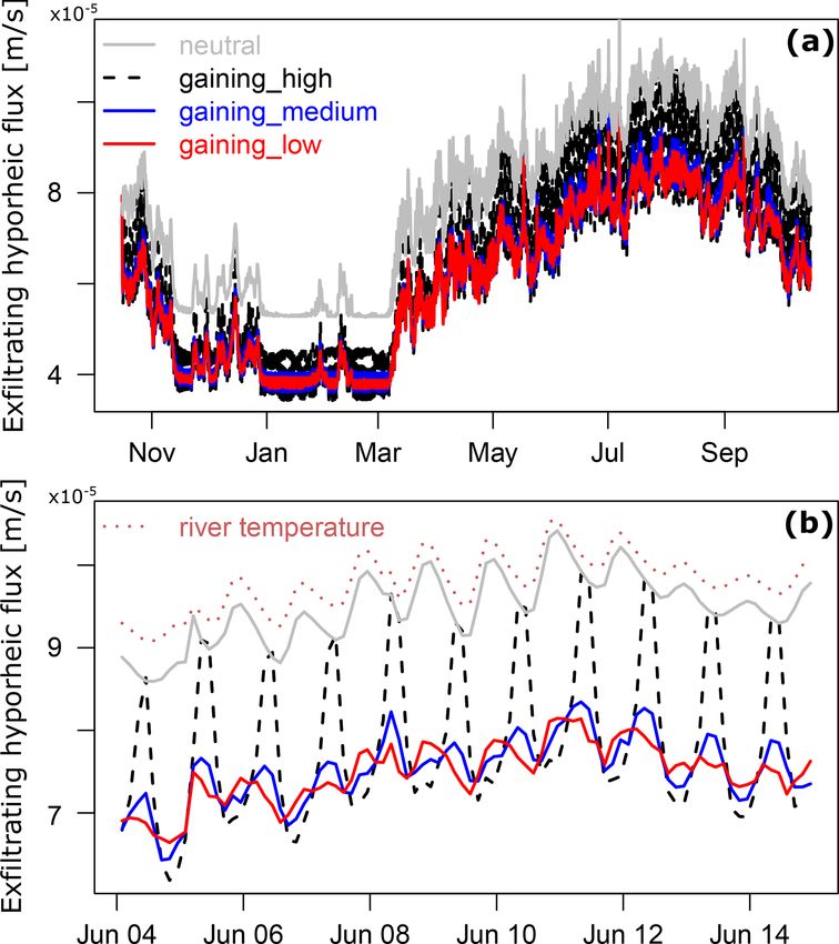
1908 L. Wu et al.: How daily groundwater table drawdown affects the diel rhythm of hyporheic exchange
Prescribed head distributions are applied at the sediment– Dirichlet and Neumann boundary is used for heat transport
water interface (Wörman et al., 2006) along the sediment–water interface. Temperature at the bot-
tom boundary is prescribed under gaining conditions. In this
2hd (t) λ
hSWI (x, t) = Hs (t) − Zbed (x) + Zbed x + , (2) case, seasonal variations in groundwater temperature (Tb ) are
1 4 assumed sinusoidal with a mean of 10 ◦ C and amplitude of
where Hs (t) [L] is the transient river stage and hd (t) is 3 ◦ C. Tb is higher than Ts in winter and lower than Ts in sum-
the dynamic head fluctuations (Fehlman, 1985; Elliott and mer. Under losing conditions, the bottom boundary is repre-
Brooks, 1997) sented by a pure convection of heat boundary.
3/8
1 2.2.3 Coupling groundwater flow and heat transport
2 for H1 ≤ 0.34
Us (t) 0.34Hs (t) s (t)
hd (t) = 0.28 3/2 (3)
2g 1
for 1 > 0.34 Transport of flow and heat in porous media is coupled by the
0.34Hs (t) Hs (t)
equations of state for density and viscosity (Furbish, 1996):
with the mean velocity Us (t) = M −1 Hs (t)2/3 S 1/2 estimated µ(T ) = m5 T 5 + m4 T 4 + m3 T 3 + m2 T 2 + m1 T + m0 (5a)
with the Chezy equation for a rectangular channel with ρ(T ) = ρ0 − ρ0 α(T − T0 ), (5b)
slope S [–] and Manning coefficient M [L−1/3 T] (Dingman,
where viscosity is in Pa s, temperature is in ◦ C,
m5 =
2009).
In the present study, an aspect ratio (the ratio between −3.916×10⁻¹³ , m4 = 1.300×10⁻¹⁰ , m3 = −1.756×10⁻⁸ ,
amplitude and wavelength 1/λ) of 0.1 and slope of 0.01 m2 = 1.286×10⁻⁶ , m1 = −5.895×10⁻⁵ , and m0 = 1.786×
are used to describe the geomorphological setting as dunes 10−3 . The reference density and temperature are ρ0 =
(Dingman, 2009; Bridge, 2009). A Manning coefficient of 1000 kg m−3 and T0 = 20 ◦ C, respectively, and the thermal
0.05 is chosen. Although this two-dimensional conceptual- expansion coefficient is α = 2.067 × 10⁻⁴ ◦ C−1 .
ization is simple in nature, it allows us to capture the hydro-
2.3 Model for mean residence time
dynamic effects on hyporheic exchange based on empirical
approaches. A comprehensive discussion on the effect of lo- We use the mean residence time to describe the time that wa-
cal morphology (i.e., aspect ratios), channel slope, and sedi- ter is exposed to biogeochemical reactive sediments (Gomez-
ment heterogeneity on the transient hydraulic pressure prop- Velez and Wilson, 2013):
agation within hyporheic zones can be found in Wu et al.
(2018). ∂a1
θ = ∇ · (D∇a1 ) − ∇ · (qa1 ) + θ a0 (6a)
∂t
2.2.2 Model for heat transport a1 (x, t) = 0 for ∂in,SWI (6b)
n · (D∇a1 ) = 0 for ∂out,SWI (6c)
Transport of heat in porous media is described by using the
heat transport equation (Bejan, 1993; Nield and Bejan, 2013) a1 (xu , y, t) = a1 (xd , y, t) for ∂u and ∂d (6d)
a1 (x, t) = a1b on ∂b under gaining condition (6e)
∂T
= ∇ · (DT ∇T ) − ∇ · (v T T ) (4a) n · (D∇a1 ) = 0 on ∂b under losing condition, (6f)
∂t
T (x, t) = Ts for ∂in,SWI (4b) where a1 (x, t) is the mean of the residence time distribution
n · (DT ∇T ) = 0 for ∂out,SWI (4c) [T], t is time [T], x = (x, y) is the spatial location vector, q
is the Darcy flux [LT−1 ], and D is the dispersion–diffusion
T (x = −L, y) = T (x = 2L, y) for ∂u and ∂d (4d)
tensor defined by Bear (1972), a0 = 1 is the initial condition
T (x, t) = Tb for ∂b under gaining condition (4e) for the moments, and a1b is the mean residence time of the
n · (DT ∇T ) = 0 for ∂b under losing condition, (4f) groundwater fluid [T−1 ]. a1b is prescribed, similar to Gomez-
Velez et al. (2014), and a value of 10 years is assumed based
where T is temperature [2], v T = (ρf cf )/(ρc)q is the ther- on Mcguire and Mcdonnell (2006).
mal front velocity [LT−1 ], DT is the hydrodynamic thermal
dispersion tensor [L2 T−1 ] calculated following Wu et al. 2.4 Defining hyporheic zones
(2020), ρc = θ ρf cf + (1 − θ )ρs cs is the specific volumetric
heat capacity of the fluid-grains media [ML−1 T−2 2−1 ], In the present study, the hyporheic zone is defined as the
ρf cf is the specific volumetric heat capacity of the fluid sediment area containing at least 90 % of the surface wa-
[ML−1 T−2 2−1 ], ρs cs is the specific volumetric heat capac- ter (Triska et al., 1989; Gooseff, 2010). A numerical tracer
ity of the solids [ML−1 T−2 2−1 ], and Ts is the temperature is simulated with an advection–dispersion equation and flow
of the water column [2], which is the measured river tem- transport model simultaneously to define the boundary of hy-
perature time series. ∂in,SWI and ∂out,SWI represent the porheic zones:
boundaries where surface water flows into and out of the sed- ∂C
iment at the sediment–water interface, respectively. A mixed θ = ∇ · (D∇C) − ∇ · (qC), (7)
∂t
Hydrol. Earth Syst. Sci., 25, 1905–1921, 2021 https://doi.org/10.5194/hess-25-1905-2021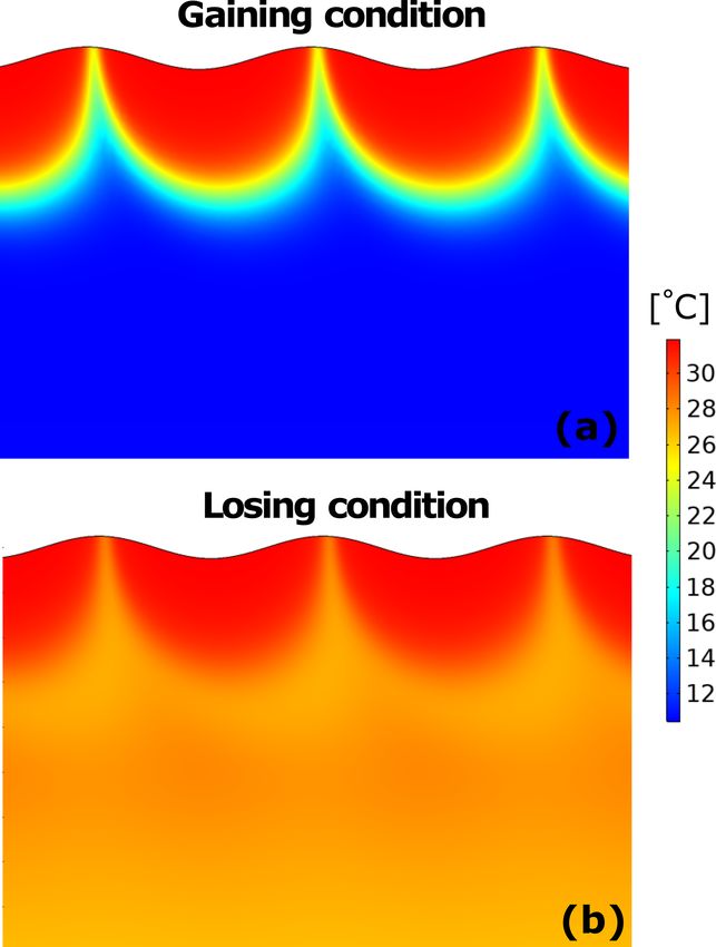
L. Wu et al.: How daily groundwater table drawdown affects the diel rhythm of hyporheic exchange                                         1909

Figure 2. Model geometry and scenarios. (a) Schematic representation of the sediment domain. The top boundary is sinusoidal with ampli-
tude 1 and wavelength λ. Lateral boundaries are periodic, representing an infinite domain in the longitudinal direction. Groundwater enters
(gaining condition, qb (+)) or leaves (losing condition, qb (−)) the domain through the bottom boundary. (b) In-phase groundwater conditions
with three amplitudes of groundwater level fluctuations. The in-phase conditions mean that the strongest groundwater fluxes occur around
the same time of the day as the highest river temperature. (c) The out-of-phase groundwater conditions, i.e., the strongest groundwater fluxes,
occur almost simultaneously with the lowest river temperatures. Temperature time series are obtained from the U.S. Geological Survey
(USGS, Site ID: 06893970). Groundwater flux is conceptualized as sinusoidal curves with varying amplitudes representing the strength of
the groundwater upwelling or downwelling and varying phases representing in-phase and out-out-phase scenarios. For figure clarity, a 10 d
time window is selected arbitrarily from 21 to 30 June 2017.

where C is the concentration of the non-reactive tracer                   porheic fluxes and water flow out of the hyporheic zone is
[ML−3 ], q is the Darcy flux [LT−1 ], and D = {Dij } is the               defined as the exfiltrating hyporheic fluxes.
dispersion–diffusion tensor defined as Bear (1972). The con-
centration of tracer in the surface water column is assumed               2.5   Study scenarios
to be Cs . Therefore, the hyporheic zone is defined when
C ≥ 0.9Cs in the sediment. The boundary of the hyporheic                  To better focus on the effect of river temperature and ground-
zone is renewed at every time point and therefore it changes              water table dynamics on hyporheic exchange, we use the ob-
over time under varying flow conditions. With this condition,             served river discharge and temperature measurements from
the threshold C ≥ 0.9Cs will eventually be exceeded across                the USGS gauging station (ID: 06893970). The gauging sta-
the entire domain under losing conditions. Therefore, the hy-             tion is located in Spring Branch Creek at Holke Road in In-
porheic zone is tracked using reversed Darcy flow in order                dependence, Missouri (lat 39◦ 050 1800 , long 94◦ 200 3600 ; ref-
to identify the areas with the largest influence from the sur-            erenced to North American Datum of 1927). The station is
face water under losing conditions. Using this definition, wa-            on the upstream left bank of Missouri Highway 78 about
ter flow into the hyporheic zone is defined as infiltrating hy-           2.4 km above the confluence with the Little Blue River with
                                                                          a drainage area of 22 km2 . The observation period is from

https://doi.org/10.5194/hess-25-1905-2021                                               Hydrol. Earth Syst. Sci., 25, 1905–1921, 2021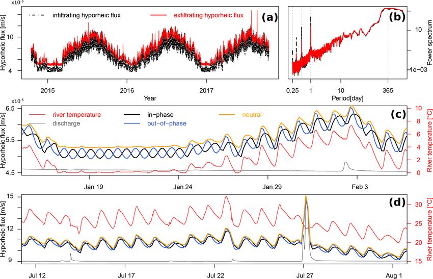
1910                 L. Wu et al.: How daily groundwater table drawdown affects the diel rhythm of hyporheic exchange

16 October 2014–16 October 2017. Spectral analysis, pre-            est fluctuation amplitude is two times higher than the sce-
sented in a previous study, shows that the river temperature        nario with medium amplitude and four times higher than the
of this site has a clear daily fluctuation pattern, whereas the     scenario with low amplitude. Using the method proposed in
river discharge exhibits no daily fluctuations (the “reference      Boano et al. (2008), which is described in detail in the Sup-
site” in Fig. 5 presented in Wu et al., 2020). Therefore, this      plement, a change in the head difference (dh) of 3.5 cm is ob-
site is an ideal site to explore the interactions of groundwater    served with the highest groundwater level fluctuation ampli-
table dynamics and river temperature fluctuations on daily          tude, where qb varies daily from 1 × 10⁻³ to 9 × 10⁻³ m s−1 .
scales without the additional influence of daily river stage        With the medium groundwater level fluctuation amplitude,
changes.                                                            the change in the head difference dh is 1.8 cm. With the low-
   Daily groundwater table drawdown due to phreatophyte-            est groundwater level fluctuation amplitude, the change in
induced water uptake mainly takes place in the afternoon            the head difference dh is 0.9 cm. These values are within a
when transpiration processes are strongest due to high air and      reasonable range for groundwater table fluctuations induced
river temperature, while agricultural, residential, or industrial   by plant water use (Butler et al., 2007). For simplicity, the
water supply may cause water table drawdown at any time             same values of groundwater fluxes are also applied to losing
during the day. Since the objective of the present study is to      systems.
explore the impacts of daily groundwater table drawdowns               Regardless of plant water uptake or anthropogenic ac-
and diel river temperature fluctuations, the study focuses on       tivities (i.e., irrigation, municipal, or industrial water sup-
two special cases: in-phase and out-of-phase conditions. In         ply), seasonal variations of groundwater fluxes cannot be
the in-phase conditions, the highest hydraulic gradient be-         neglected. For instance, a gradual transition of the phreato-
tween the surface water and groundwater table (strongest            phyte’s dormancy in fall often induces a progressive dimin-
groundwater flux) occurs around the same time of the day            ishing in diurnal fluctuations and changes in the multi-day
as the occurrence of the highest river temperature; in the out-     trend in groundwater tables (Butler et al., 2007). Irrigation
of-phase conditions, the highest hydraulic gradient between         activities also follow the different seasonal water demand of
surface water and groundwater (strongest groundwater flux)          agricultural plants. However, these seasonal changes are hard
occurs around the same time of the day as the occurrence            to generalize because groundwater flux variability depends
of the lowest river temperature (Fig. 2b and c). Under gain-        on a variety of factors such as plant types, water availabil-
ing scenarios, out-of-phase conditions represent the natural        ity, and local climate conditions. Understanding the effect of
state that the highest air and river temperature occurs at the      seasonal groundwater variability is beyond the scope of the
lowest water table (resulting in the lowest groundwater flow        present study. Therefore, a uniform fluctuation amplitude of
rate) in the aquifer due to transpiration by vegetation; un-        groundwater fluxes in the studied period is used.
der losing scenarios, in-phase conditions represent a scenario
driven by transpiration, because the highest air and river tem-
perature contributes to the strongest transpiration, which re-      3     Results
sults in a larger hydraulic head difference between river and
                                                                    In the observation period, the river discharge is intermit-
aquifer, and thus contributes to the higher losing groundwa-
                                                                    tent and characterized by short recession periods (approxi-
ter fluxes. The objective of this study is not to understand
                                                                    mately from 2 to 1500 m3 s−1 ); the river temperature shows
groundwater responses to pumping activities. Even though
                                                                    clear seasonal variations (approximately from 0 to 35 ◦ C) and
the timing of groundwater table drawdown depends on mul-
                                                                    daily fluctuations. Mean annual precipitation at the gauge lo-
tiple factors, i.e., the hydrological connectivity between wells
                                                                    cation is 106 cm. Average annual air temperature at the gauge
and aquifer, aquifer properties for plant water use, and pump-
                                                                    location is 12.6 ◦ C. There is no dam in the watershed.
ing capacity and electricity tariff for anthropocentric pump-
ing activities, the two special cases, namely in-phase and out-     3.1     Hyporheic fluxes
of-phase groundwater conditions, can capture the representa-
tive dynamic hyporheic responses to different timing of daily       3.1.1    Under neutral conditions
groundwater withdrawal under corresponding river tempera-
ture conditions.                                                    Under neutral conditions, exfiltrating hyporheic fluxes (the
   Groundwater flow fluctuations, as a response to daily            red solid line in Fig. 3a) present similar temporal variations
groundwater table drawdown, are conceptualized as sinu-             as infiltrating hyporheic fluxes (the black dot-dash line in
soidal curves with varying amplitudes and phases. Differ-           Fig. 3a). The diel fluctuations of exfiltrating hyporheic fluxes
ent phases reflect different timing of daily groundwater with-      (the orange solid line in Fig. 3e and f) follow the diel river
drawal, represented by the in-phase and out-of-phase ground-        temperature fluctuations (the red solid line in Fig. 3e and f).
water flow conditions as described above. Different am-             In winter, when the river temperature (the red solid line in
plitudes represent different intensities of groundwater table       Fig. 3e) is relatively stable (around 20 January), the exfiltrat-
drawdowns. For gaining system, three degrees of groundwa-           ing hyporheic fluxes also have negligible daily fluctuations;
ter table fluctuation amplitudes are investigated. The high-        when the temperature gets higher, the exfiltrating hyporheic

Hydrol. Earth Syst. Sci., 25, 1905–1921, 2021                                        https://doi.org/10.5194/hess-25-1905-2021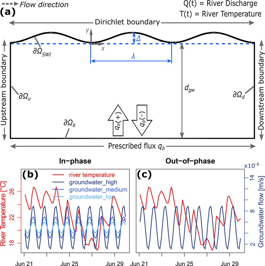
L. Wu et al.: How daily groundwater table drawdown affects the diel rhythm of hyporheic exchange                                  1911

fluxes start to fluctuate following the diel fluctuations of river   filtrating hyporheic fluxes, with decreasing groundwater up-
temperature.                                                         welling amplitude, the peaks of exfiltrating hyporheic fluxes
                                                                     (the black dash line, blue solid line, and red solid line in
3.1.2   Under gaining conditions                                     Fig. 4b) are shifted towards the patterns that coincide more
                                                                     with diel river temperature fluctuations (the dash line in
Compared to neutral conditions, groundwater upwelling                Fig. 4b) and hyporheic fluxes under neutral conditions (gray
leads to an increase of daily fluctuations of exfiltrating hy-       solid line). In other words, with decreasing groundwater ta-
porheic fluxes. Under gaining conditions, exfiltrating hy-           ble fluctuation amplitude, river temperatures exhibit stronger
porheic fluxes (the red solid line in Fig. 3c) present larger        controls on the phase of hyporheic flux diel fluctuations.
daily amplitude variations than infiltrating hyporheic fluxes            Effects of groundwater table fluctuation amplitudes on dy-
(the black dot-dash line in Fig. 3c). These observations are         namic hyporheic responses are only explored under in-phase
reflected in the frequency domain using a power spectrum.            scenarios because under out-of-phase scenarios fluctuations
For neutral conditions, infiltrating and exfiltrating hyporheic      of exfiltrating hyporheic fluxes are almost always in the same
fluxes show similar spectral power on both annual and daily          phase as the diel river temperature fluctuations. Therefore,
scales (Fig. 3b), whereas for gaining conditions, the spectral       unlike in-phase scenarios, the phase shifts due to reduced am-
power of exfiltrating hyporheic fluxes (the red solid line in        plitudes in groundwater table fluctuation are not observed.
Fig. 3d) at daily scales are markedly higher than the spectral       Reduced amplitudes in groundwater table fluctuation un-
power of infiltrating hyporheic fluxes (the black dot-dash line      der out-of-phase scenarios only contribute to reduced ampli-
in Fig. 3d).                                                         tudes in exfiltrating hyporheic flux fluctuations. For simplic-
   With gaining groundwater fluxes, the fluctuation pattern of       ity, only the results of in-phase scenarios are presented in
hyporheic fluxes changes substantially. Even with negligible         Fig. 4.
diel fluctuations of river temperature (around 20 January), the
exfiltrating hyporheic fluxes still present clear daily fluctua-
                                                                     3.1.3   Under losing conditions
tions following the groundwater drawdown as indicated by
the opposite fluctuating patterns between the exfiltrating hy-
porheic fluxes under in-phase (the black line in Fig. 3e and f)      Unlike gaining conditions, under losing conditions the fluc-
and out-of-phase (the blue line in Fig. 3e and f) groundwater        tuation amplitudes of exfiltrating hyporheic fluxes are re-
scenarios. When the temperature gets higher, the groundwa-           duced compared to infiltrating hyporheic fluxes (Fig. 5a).
ter table drawdown-induced hyporheic fluctuations are main-          This is also revealed in the frequency domain where the
tained. The exfiltrating hyporheic fluxes under the in-phase         spectral power of exfiltrating hyporheic fluxes is reduced at
scenario have an opposite fluctuation pattern to the exfiltrat-      daily scales compared to the spectral power of infiltrating hy-
ing hyporheic fluxes under the out-of-phase scenario, river          porheic fluxes (Fig. 5b).
temperature, and the exfiltrating hyporheic fluxes under neu-           The river temperature also demonstrates different impacts
tral conditions; the exfiltrating hyporheic fluxes under the         under losing conditions. In winter, when the river tempera-
out-of-phase scenario fluctuate with river temperature. It is        ture (the red solid line in Fig. 5c) is relatively stable (around
worth noting that the peaks of exfiltrating hyporheic fluxes         20 January), the exfiltrating hyporheic fluxes under in-phase
under the out-of-phase scenario are slightly higher than the         and out-of-phase groundwater drawdown conditions exhibit
peaks of exfiltrating hyporheic fluxes under the in-phase sce-       an opposite fluctuation pattern resulting from the different
nario at a warm temperature (Fig. 3f).                               timing of groundwater table drawdown (black and blue solid
   On 27 July, under the same flood event that causes a dis-         lines). This observation is the same with gaining conditions
charge increase from 2 to 1500 m3 s−1 (the gray solid line           (Fig. 3e). However, when the river temperature gradually in-
in Fig. 3f), exfiltrating hyporheic fluxes increase much more        creases, the phase differences between the diel fluctuations
under the in-phase scenario (the black solid line) than under        of exfiltrating hyporheic fluxes under in-phase and out-of-
the out-of-phase scenario (the blue solid line). The increase        phase scenarios are diminishing. In summer, when river tem-
of exfiltrating hyporheic fluxes under the in-phase scenario is      perature is relatively high, exfiltrating hyporheic fluxes un-
nearly two times as high as the increase of hyporheic fluxes         der in-phase and out-of-phase conditions are fluctuating with
under the out-of-phase scenario.                                     almost the same phase as the river temperature (Fig. 5d).
   To explore the impact of groundwater table fluctuation am-        This observation is in great contrast to the gaining condition
plitudes on dynamic hyporheic responses, groundwater ta-             where the opposite fluctuation patterns between exfiltrating
ble fluctuations with three different amplitudes are applied to      hyporheic fluxes under in-phase and out-of-phase conditions
simulate hyporheic exchange processes under in-phase sce-            are kept from winter to summer (Fig. 3f).
narios (as the groundwater scenarios plotted in Fig. 2b). With          Unlike gaining conditions, on 27 July under the same flood
the reduced groundwater upwelling amplitudes, the ampli-             event (the gray solid line in Fig. 5d), the increases of exfiltrat-
tudes of exfiltrating hyporheic flux fluctuations are also re-       ing hyporheic fluxes under in-phase and out-of-phase scenar-
duced (Fig. 4a). More than the amplitude reduction of ex-            ios are similar. These distinctions indicate a vastly different

https://doi.org/10.5194/hess-25-1905-2021                                          Hydrol. Earth Syst. Sci., 25, 1905–1921, 2021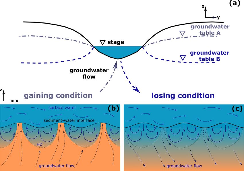
1912 L. Wu et al.: How daily groundwater table drawdown affects the diel rhythm of hyporheic exchange
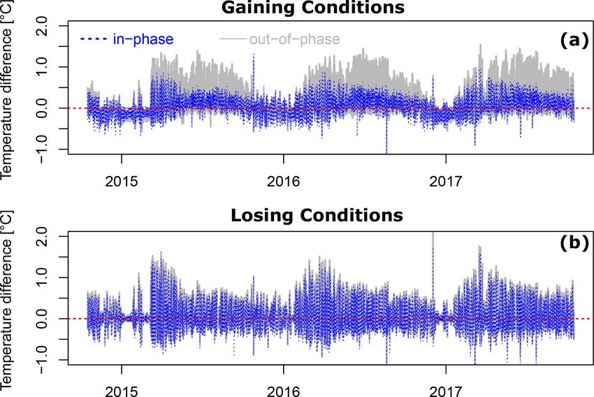
Figure 3. Effect of diel river temperature fluctuations and daily groundwater table drawdowns on hyporheic fluxes under gaining conditions.
Infiltrating and exfiltrating hyporheic fluxes under (a) neutral and (c) gaining conditions. Power spectrum of infiltrating and exfiltrating
hyporheic fluxes under (b) neutral and (d) gaining conditions. Exfiltrating hyporheic fluxes under neutral conditions and under gaining
conditions with in-phase and out-of-phase groundwater drawdown scenarios in (e) winter and (f) summer. For figure clarity, discharge is not
scaled in (e) and (f) but used only for qualitative comparisons. The flood event on 27 July causes a discharge increase from 2 to 1500 m3 s−1 .
coupled flow and heat transport pattern between gaining and of exfiltrating hyporheic fluxes; negative values indicate a
losing systems. higher temperature of exfiltrating hyporheic fluxes. Under
gaining conditions, seasonal variations are observed for both
3.2 Heat transport in hyporheic zones in-phase and out-of-phase conditions. In winter, the exfiltrat-
ing hyporheic fluxes are generally warmer than the river; in
Snapshots of temperature distributions in the sediment summer, the river is generally warmer than the exfiltrating
demonstrate noticeable differences in the heat transport hyporheic fluxes. These seasonal variations are more promi-
under different groundwater conditions on a summer day nent under out-of-phase conditions (the gray solid line in
(22 July 2017 at 17:00) (Fig. 6). Under gaining conditions, Fig. 7a) than under in-phase conditions (the blue dashed line
both river and groundwater temperature play important roles in Fig. 7a). In summer, the exfiltrating hyporheic fluxes un-
in determining the temperature of the sediment, whereas un- der out-of-phase conditions are much cooler than river wa-
der losing conditions only the river temperature affects the ter compared to the in-phase conditions. Under losing con-
temperature distributions in the sediment. ditions, the differences between in-phase and out-of-phase
Temperature differences between river and exfiltrating hy- conditions are not as significant as under gaining conditions
porheic fluxes are explored for both gaining and losing, and (Fig. 7b).
in-phase and out-of-phase conditions (Fig. 7). Positive val-
ues indicate a higher river temperature than the temperature
Hydrol. Earth Syst. Sci., 25, 1905–1921, 2021 https://doi.org/10.5194/hess-25-1905-2021L. Wu et al.: How daily groundwater table drawdown affects the diel rhythm of hyporheic exchange 1913
Under gaining conditions, RSFa displays opposite diel
variations between the in-phase and out-of-phase scenarios.
Significant drops occur during flood events. Under losing
conditions, RSFa is around 3.5 orders of magnitude lower
than under gaining conditions. Daily-scale variations be-
tween in-phase and out-of-phase scenarios under losing con-
ditions are less significant than under gaining conditions.
4 Discussion
4.1 Groundwater modifies the variability of hyporheic
exchange rates
With daily groundwater table drawdowns, additional hy-
draulic gradient changes on a daily scale contribute to en-
hanced diel fluctuations of hyporheic fluxes. Under neutral
conditions, similar diel fluctuation patterns in both infiltrat-
ing and exfiltrating hyporheic fluxes (Fig. 3a and b) are
mainly due to the change of hydraulic conductivity, which
is a function of diel temperature fluctuations. Unlike neu-
tral conditions, under gaining conditions the exfiltrating hy-
porheic fluxes show enhanced fluctuation amplitudes com-
Figure 4. Effect of amplitudes in groundwater level fluctuations pared to the infiltrating hyporheic fluxes due to the addi-
on hyporheic fluxes. (a) Exfiltrating hyporheic fluxes under neutral tional fluctuations in the gaining groundwater fluxes that are
and gaining groundwater fluxes with three different amplitudes. (b) mixed with the hyporheic fluxes that originate from the sur-
Comparisons of daily fluctuation phases among river temperature face (Fig. 3c and d). Under losing conditions, the infiltrating
and exfiltrating hyporheic fluxes under neutral and gaining ground- hyporheic fluxes have higher fluctuation amplitudes because
water fluxes with three different amplitudes. there is no mixing in the exfiltrating hyporheic fluxes under
losing conditions as the mixing occurred under gaining con-
3.3 Reaction significance factor ditions according to the geochemical definitions of hyporheic
zones (Fig. 5a and b). Under both gaining and losing con-
Denitrification potential in hyporheic zones can be quanti- ditions, the exfiltrating hyporheic fluxes exhibit higher fluc-
fied using the reaction significance factor (RSF). The RSF tuation amplitudes than under neutral conditions, indicating
is calculated as the ratio between hyporheic mean residence groundwater table dynamics contribute to additional fluctua-
time and a characteristic timescale for denitrification and tions in the hyporheic exchange fluxes.
then scaled by the proportion of the river discharge passing The timing of groundwater table drawdown also affects
the hyporheic zone (Harvey et al., 2013). In the present study, hyporheic exchange rates. For instance, under the same flood
we use the RSF calculated as the value per unit bedform area event on 27 July (the gray solid line in Fig. 3f), the ex-
(denoted by the subscript “a”): filtrating hyporheic flux under in-phase gaining conditions
qHZ τHZ (the black solid line) increases more than the exfiltrating hy-
RSFa = · , (8) porheic flux under out-of-phase conditions (the blue solid
Q τdn
line). This is because the groundwater gaining flux under the
where qHZ is the exfiltrating hyporheic fluxes [LT−1 ], Q is in-phase scenario is lowest in the course of the day when
the river discharge [L3 T−1 ], τHZ is the mean of the proba- the flood arrives, whereas it is highest under the out-of-phase
bility distribution of the residence time at any time point [T], scenario. As a result of higher groundwater upward pressure,
and τdn is the characteristic timescale for denitrification [T]. higher groundwater upwelling flow under the out-of-phase
Typical timescales of denitrification in hyporheic zones are scenario compresses the hyporheic zone extension during the
reported by Gomez-Velez and Harvey (2014); Gomez-Velez flood event. Consequently, exfiltrating hyporheic fluxes un-
et al. (2015) and the quantiles are used in the calculation. The der in-phase conditions increase twice as much as exfiltrating
25th, 50th, and 75th quantiles are presented in Fig. S1 in the hyporheic fluxes under out-of-phase conditions. In contrast,
Supplement. It is worth noting that instead of denitrification, the differences of exfiltrating hyporheic fluxes between in-
reaction potential of a different geochemical process can be phase and out-of-phase scenarios are marginal in response to
assessed if a different characteristic timescale is applied in the same flood event under losing conditions (Fig. 5d). The
Eq. (8). reasons will be explored in the following section.
https://doi.org/10.5194/hess-25-1905-2021 Hydrol. Earth Syst. Sci., 25, 1905–1921, 20211914 L. Wu et al.: How daily groundwater table drawdown affects the diel rhythm of hyporheic exchange
Figure 5. Effect of diel river temperature fluctuations and daily groundwater table drawdowns on hyporheic fluxes under losing conditions.
(a) Infiltrating and exfiltrating hyporheic fluxes under losing conditions and (b) corresponding power spectrum. Exfiltrating hyporheic fluxes
under neutral conditions and under losing conditions with in-phase and out-of-phase groundwater drawdown scenarios in (c) winter and
(d) summer. For figure clarity, discharge is not labeled in (c) and (d). The flood event on 27 July causes a discharge increase from 2 to
1500 m3 s−1 .
This observation has potential implications on optimizing groundwater table dynamics are critical for water manage-
aquifer pumping schedules. Hypothetically, if the rising dis- ment agencies to minimize the environmental footprint of the
charge is from an untreated wastewater discharge source, the withdrawal process.
timing of the groundwater table drawdown will significantly
affect the spreading and mixing of pollutants in the sedi- 4.2 Different impacts of groundwater on hyporheic
ment. At the moment of flood events, more pollutants will be exchange under gaining and losing systems
carried into the sediment with a higher hyporheic exchange
rate under a relatively low upwards-directed pressure of the The timing of groundwater table drawdown has substan-
groundwater than under a relatively high upwards-directed tially different impacts on hyporheic exchange processes un-
pressure. Therefore, the timing of the aquifer pumping can der gaining and losing conditions in different seasons. More
potentially amplify or reduce the dispersal of pollutants in specifically, under gaining conditions, the opposite phases
the aquifer. of groundwater table fluctuations under in-phase and out-
Modern regulating reservoirs are usually designed with of-phase conditions induce an opposite fluctuation pattern of
enough storage capacities allowing planning of pumping exfiltrating hyporheic fluxes in both winter and summer (the
schedules independent of user demand (Reca et al., 2014). black and blue solid lines in Fig. 3e and f). However, un-
A poorly designed pumping regime is detrimental to the bi- der losing conditions the opposite fluctuation patterns of ex-
ological and ecological functioning of the fluvial systems filtrating hyporheic fluxes under in-phase and out-of-phase
(Moore, 1999; Libera et al., 2017; Bredehoeft and Kendy, conditions gradually disappear with increasing river temper-
2008). Consequently, careful selection of aquifer pumping atures from winter to summer (the black and blue solid lines
schedules with considerations of both timing of flood and in Fig. 5c and d). Unlike gaining conditions, under losing
conditions exfiltrating hyporheic fluxes in both the in-phase
Hydrol. Earth Syst. Sci., 25, 1905–1921, 2021 https://doi.org/10.5194/hess-25-1905-2021L. Wu et al.: How daily groundwater table drawdown affects the diel rhythm of hyporheic exchange 1915
With the temperature variation approximately from 0 to
30 ◦ C, viscosity decreases by 45 % and hydraulic conductiv-
ity increases by 220 % (Wu et al., 2020). Therefore, in sum-
mer when river temperature is relatively high, the hydraulic
conductivity is enhanced and becomes the main modulator
for hyporheic exchange rate under losing conditions. Com-
pared to hydraulic conductivity, the effect of daily fluctu-
ations of groundwater gradients becomes less important in
determining the variability of hyporheic exchange processes.
Consequently, the differences of exfiltrating hyporheic fluxes
between in-phase and out-of-phase losing conditions disap-
pear in summer. This also explains the different effects of
the timing of groundwater table drawdowns during the same
flood event on 27 July under gaining (Fig. 3f) and losing
conditions (Fig. 5d). Unlike gaining conditions, under losing
conditions the differences between flood-induced increases
of exfiltrating hyporheic fluxes in in-phase and out-of-phase
scenarios are negligible, because river temperatures have a
more dominant role in determining the variability of hy-
porheic exchange fluxes under losing systems.
Figure 6. Snapshots of temperature distributions in the sediment on It is noteworthy that when river temperature is rela-
22 July 2017 at 17:00 for (a) gaining and (b) losing groundwater tively high, the exfiltrating hyporheic fluxes under out-of-
conditions.
phase gaining conditions fluctuate with a higher amplitude
(Fig. 3f). This is because under gaining out-of-phase scenar-
ios, a lower groundwater table (lower groundwater upwelling
and out-of-phase scenarios present an almost synchronized fluxes) occurs in the afternoon when the river temperature is
fluctuation pattern following the diel river temperature fluc- relatively high. Both a low groundwater upward gradient and
tuations in summer. These results indicate that under los- a high river temperature promote hyporheic exchange. Con-
ing conditions both river temperature and the timing of the sequently, the exfiltrating hyporheic fluxes fluctuate with a
groundwater table drawdown affect the phase of exfiltrating higher amplitude under out-of-phase gaining conditions than
hyporheic flux fluctuations in winter, when river tempera- under in-phase conditions.
tures are relatively low; river temperature, however, plays When gradually reducing the groundwater fluctuation am-
a more dominant role in determining the phase of the hy- plitudes, the crests of exfiltrating hyporheic fluxes under
porheic flux fluctuations in summer, when river temperatures in-phase gaining groundwater scenarios shift from the tim-
are relatively high. In other words, higher river temperature ing of river temperature troughs to river temperature peaks
has larger impacts on the temporal variations of hyporheic (Fig. 4b). This is additional clear evidence that both diel
exchange. river temperatures and groundwater daily fluctuations regu-
To better understand the causes of different hyporheic late the phases and amplitudes of hyporheic exchange fluxes:
responses under gaining and losing conditions with rela- when the groundwater fluxes are small, the diel rhythm of
tively high river temperatures (i.e., in summer), snapshots hyporheic flux fluctuations is following the diel fluctuations
of sediment temperature distributions on a summer after- of river temperature, whereas when the groundwater fluxes
noon are presented (Fig. 6). Under gaining conditions, ar- increase, the diel rhythm of hyporheic flux fluctuations is fol-
eas affected by the river temperature are closely dependent lowing the timing of groundwater level daily drawdown.
on the hyporheic exchange processes (Fig. 6a). When the
hyporheic exchange rate is low, the river temperature has a 4.3 Groundwater modifies hyporheic buffering effects
negligible effect on the sediment hydraulic conductivity be- on temperature
cause the heat advection of upwelling groundwater is domi-
nant. When hyporheic exchange rates are relatively high, hy- Temperature differences between river and exfiltrating hy-
porheic zones will extend deeper and wider in the sediment porheic fluxes also demonstrate distinct patterns between
and river bank (Gomez-Velez et al., 2017; Wu et al., 2018). gaining and losing, and in-phase and out-of-phase condi-
As a consequence, river temperature will have a larger impact tions. Under gaining conditions, the temperature differences
on the sediment hydraulic conductivity. Under losing condi- display negative values in winter periods and positive values
tions, however, the sediment hydraulic conductivity is pre- in summer periods due to the mixing between surface water
dominantly affected by the surface water heat advection and and groundwater (Fig. 7a). In winter, the groundwater is of-
conduction (Fig. 6b). ten warmer than surface water, while in summer the ground-
https://doi.org/10.5194/hess-25-1905-2021 Hydrol. Earth Syst. Sci., 25, 1905–1921, 20211916 L. Wu et al.: How daily groundwater table drawdown affects the diel rhythm of hyporheic exchange Figure 7. Temperature differences between river and exfiltrating hyporheic fluxes under (a) gaining and (b) losing in-phase and out-of-phase fluctuations of diel river temperature and daily groundwater table drawdown. water is often colder than surface water. Therefore, tem- scheduling the pumping activities in order to protect thermal perature differences under gaining conditions demonstrate a heterogeneity across multiple spatial scales. clear seasonal fluctuations around zero. Unlike gaining con- ditions, temperature differences under losing conditions have 4.4 Groundwater modifies hyporheic potential for no clear seasonal fluctuations around the value zero due to biogeochemical reactions the limited mixing between regional groundwater and sur- face water. Hyporheic potential for denitrification varies between gain- The temperature differences between exfiltrating hy- ing and losing, and in-phase and out-of-phase conditions porheic fluxes between in-phase and out-of-phase gaining (Fig. 8). RSFa displays substantial drops during flood events. conditions are directly related to the temporal variability of This is because the flood-induced hydraulic gradient in- hyporheic exchange fluxes (Fig. 3e and f) and sediment tem- creases at the sediment–water interface, drives more surface perature distribution. As discussed above, the hyporheic ex- water into the sediment, and consequently accelerates hy- change rate is higher under out-of-phase conditions than un- porheic exchange rates. Increased hyporheic exchange rates der in-phase conditions when river temperatures are rela- lead to a substantial decrease of the residence time in the tively high. As a result, the hyporheic zone has a larger exten- hyporheic zone, creating conditions less suitable for denitri- sion and surface water can infiltrate deeper into the sediment. fication. Similarly, RSFa under gaining conditions is around Therefore, hyporheic zones have a larger cooling effect dur- 3 orders of magnitude higher than under losing conditions ing high river temperature under out-of-phase gaining condi- due to the significantly longer residence time resulting from tions than under in-phase gaining conditions. mixing between surface water and groundwater under gain- Spatial variability in river and sediment temperature may ing conditions. provide localized refugia against extreme thermal distur- With groundwater gaining conditions, RSFa peaks at dif- bances for aquatic communities (Berman and Quinn, 1991). ferent times during a day under in-phase and out-of-phase Loss of these refugia increases the risk for organisms liv- scenarios, indicating hyporheic denitrification potential can ing under undesirable temperatures associated with diel tem- be regulated by adjusting the timing of daily groundwater perature fluctuations and anthropogenic activities (Poole and table drawdowns. With groundwater losing conditions, even Berman, 2001). In the present study, we observe that the though RSFa display peaks at different times during a day timing of daily groundwater table drawdown (i.e., in-phase on a logarithmic scale under in-phase and out-of-phase sce- or out-of-phase scenarios) potentially affects the ability of narios, the actual differences of RSFa (on the scale of 10−5 ) hyporheic zones to act as temperature buffers that can sus- between in-phase and out-of-phase conditions are insignifi- tain vital activities (i.e., survival, growth, and reproduction) cant compared to gaining conditions (Fig. 8a and b). In con- for aquatic communities. Therefore, care must be taken in clusion, the timing of groundwater table drawdown is more Hydrol. Earth Syst. Sci., 25, 1905–1921, 2021 https://doi.org/10.5194/hess-25-1905-2021
L. Wu et al.: How daily groundwater table drawdown affects the diel rhythm of hyporheic exchange                                 1917

                                                                            The first term in RSFa (qHZ /Q) describing the proportion
                                                                         of river discharge passing through the hyporheic zone per
                                                                         unit bedform area can be used to quantify the connectivity
                                                                         between the river and hyporheic zone (Harvey et al., 2019).
                                                                         This connectivity underpins many ecosystem processes and
                                                                         important reactions that take place in close contact with bio-
                                                                         geochemical reactive sediments (Boulton, 2007; Ward et al.,
                                                                         2000; Malard et al., 2002; Roley et al., 2012). Maintaining
                                                                         a good hydrological connectivity is therefore crucial. Un-
                                                                         der the same river discharge rates (Q), hyporheic exchange
                                                                         rates (qHZ ) are higher when groundwater drawdown is out-
                                                                         of-phase to diel river temperature fluctuations than in-phase.
                                                                         Consequently, the hydrological connectivity is higher in an
                                                                         out-of-phase scenario. The temperature differences between
                                                                         river and exfiltrating hyporheic fluxes with in-phase and out-
                                                                         of-phase groundwater table drawdown also proves this find-
                                                                         ing (Fig. 7). Hydrological connectivity is higher in out-of-
                                                                         phase groundwater table fluctuation scenarios than in in-
                                                                         phase scenarios, making the hyporheic zone a better thermal
                                                                    .    buffer under out-of-phase scenarios.
Figure 8. Reaction significance factors per unit area (RSFa ) for den-
itrification potentials from 15 to 30 May 2017. (a) RSFa under gain-     4.5   Study limitations
ing conditions. (b) RSFa under losing conditions. The results are
selected arbitrarily with the considerations of figure clarity           The aim of the present study is not to simulate hyporheic ex-
                                                                         change processes in perfect detail but rather to gain mech-
                                                                         anistic understanding of hyporheic responses to varying
important under gaining conditions than under losing condi-              groundwater table fluctuation patterns. Therefore, simplifi-
tions for denitrification reactions.                                     cations are made to allow for an efficient and reasonably
   In Harvey et al. (2019), RSF was calculated based on mean             correct representation of hyporheic exchange processes. De-
annual hyporheic flux and river discharge without consider-              tailed simplifications and limitations on model dimensional-
ations of the temporal variability of the flow conditions and            ity, geomorphological settings, and boundary conditions are
groundwater gaining or losing. To be able to compare our re-             critically reviewed in previous studies on which the develop-
sults with those results, we also calculated mean RSF using              ment of current method is based (Wu et al., 2018, 2020). In
mean river discharge and mean hyporheic fluxes. The calcu-               the following, only simplifications that are most relevant to
lated mean RSF is approximately −2.7 to −1.8 for gaining                 the present study are discussed.
conditions and −5.8 to −4.8 for losing conditions, which                    Groundwater fluxes are simplified as prescribed upward
roughly falls within the range of the mean RSF observed                  or downward fluxes. Daily groundwater table drawdowns are
in Harvey et al. (2019). Under losing conditions, the RSF                represented by sinusoidal curves with different phases and
is smaller than the values reported in Harvey et al. (2019)              amplitudes representing different timing of groundwater ta-
because losing conditions significantly reduce the denitrifi-            ble drawdowns and strength of groundwater upwelling or
cation potential as indicated in Fig. 8.                                 downwelling, respectively (Fig. 2). However, the direction
   It is worth mentioning that the observations of RSFa are              and magnitude of groundwater flow is a response to the head
not limited to denitrification processes. For a different bio-           difference between river stage and riparian water table ele-
geochemical reaction, another characteristic timescale is ap-            vation as well as sediment properties. An important process
plied instead of τdn . The results presented in Fig. 8 will only         that cannot be represented by using prescribed groundwater
be scaled by a different biogeochemical timescale for the re-            fluxes is the impact of river temperature as a major factor
action of interest. The relative variations of RSFa remain the           contributing to reduced afternoon river discharge. High river
same for other biogeochemical reactions.                                 temperature in the afternoon results in a high hydraulic con-
   The temperature-dependence of τdn is not considered;                  ductivity, which contributes to increased losing fluxes and
however, we use both the 25th and 75th quantiles as the lower            consequently a reduced afternoon river discharge (Constantz
and upper ranges for calculating RSFa , which mostly include             et al., 1994). However, increasing losing fluxes due to higher
the variations caused by the changing temperature as indi-               river temperature in the afternoon cannot be captured us-
cated in Zheng et al. (2016), where a roughly 5-fold increase            ing a prescribed groundwater flux time series. Apart from
was observed in denitrification rates when temperature in-               changing sediment hydraulic conductivity, there are a myr-
creased from 5 to 35 ◦ C.                                                iad of other factors affecting groundwater table fluctuations.

https://doi.org/10.5194/hess-25-1905-2021                                             Hydrol. Earth Syst. Sci., 25, 1905–1921, 2021
You can also read