ROBUSTNESS MAY BE AT ODDS WITH ACCURACY - OpenReview
←
→
Page content transcription
If your browser does not render page correctly, please read the page content below
Published as a conference paper at ICLR 2019

ROBUSTNESS M AY BE AT O DDS WITH ACCURACY
 Dimitris Tsipras∗, Shibani Santurkar∗, Logan Engstrom∗, Alexander Turner, Aleksander Madry
                                                                                        ˛
 Massachusetts Institute of Technology
 {tsipras,shibani,engstrom,turneram,madry}@mit.edu

                                                A BSTRACT

             We show that there exists an inherent tension between the goal of adversarial
             robustness and that of standard generalization. Specifically, training robust models
             may not only be more resource-consuming, but also lead to a reduction of standard
             accuracy. We demonstrate that this trade-off between the standard accuracy of a
             model and its robustness to adversarial perturbations provably exists even in a fairly
             simple and natural setting. These findings also corroborate a similar phenomenon
             observed in practice. Further, we argue that this phenomenon is a consequence
             of robust classifiers learning fundamentally different feature representations than
             standard classifiers. These differences, in particular, seem to result in unexpected
             benefits: the features learned by robust models tend to align better with salient data
             characteristics and human perception.

1       I NTRODUCTION
Deep learning models have achieved impressive performance on a number of challenging benchmarks
in computer vision, speech recognition and competitive game playing (Krizhevsky et al., 2012; Graves
et al., 2013; Mnih et al., 2015; Silver et al., 2016; He et al., 2015a). However, it turns out that these
models are actually quite brittle. In particular, one can often synthesize small, imperceptible perturba-
tions of the input data and cause the model to make highly-confident but erroneous predictions (Dalvi
et al., 2004; Biggio & Roli, 2017; Szegedy et al., 2013).
This problem of so-called adversarial examples has garnered significant attention recently and
resulted in a number of approaches both to finding these perturbations, and to training models that are
robust to them (Goodfellow et al., 2014b; Nguyen et al., 2015; Moosavi-Dezfooli et al., 2016; Carlini
& Wagner, 2016; Sharif et al., 2016; Kurakin et al., 2016a; Evtimov et al., 2017; Athalye et al., 2017).
However, building such adversarially robust models has proved to be quite challenging. In particular,
many of the proposed robust training methods were subsequently shown to be ineffective (Carlini
& Wagner, 2017; Athalye et al., 2018; Uesato et al., 2018). Only recently, has there been progress
towards models that achieve robustness that can be demonstrated empirically and, in some cases, even
formally verified (Madry et al., 2017; Kolter & Wong, 2017; Sinha et al., 2017; Tjeng & Tedrake,
2017; Raghunathan et al., 2018; Dvijotham et al., 2018a; Xiao et al., 2018b).
The vulnerability of models trained using standard methods to adversarial perturbations makes
it clear that the paradigm of adversarially robust learning is different from the classic learning
setting. In particular, we already know that robustness comes at a cost. This cost takes the form
of computationally expensive training methods (more training time), but also, as shown recently in
Schmidt et al. (2018), the potential need for more training data. It is natural then to wonder: Are
these the only costs of adversarial robustness? And, if so, once we choose to pay these costs, would
it always be preferable to have a robust model instead of a standard one? The goal of this work is
to explore these questions and thus, in turn, to bring us closer to understanding the phenomenon of
adversarial robustness.

Our contributions It might be natural to expect that training models to be adversarially robust,
albeit more resource-consuming, can only improve performance in the standard classification setting.
In this work, we show, however, that the picture here is much more nuanced: these two goals might
be fundamentally at odds. Specifically, even though applying adversarial training, the leading method
    ∗
        Equal Contribution.

                                                       1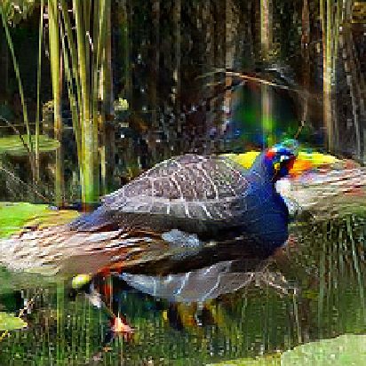
Published as a conference paper at ICLR 2019

for training robust models, can be beneficial in some regimes of training data size, in general, there is
a trade-off between the standard accuracy and adversarially robust accuracy of a model. In fact, we
show that this trade-off provably exists even in a fairly simple and natural setting.
At the root of this trade-off is the fact that features learned by the optimal standard and optimal
robust classifiers are fundamentally different and, interestingly, this phenomenon persists even in the
limit of infinite data. This thus also goes against the natural expectation that given sufficient data,
classic machine learning tools would be sufficient to learn robust models and emphasizes the need for
techniques specifically tailored to training robust models.
Our exploration also uncovers certain unexpected benefit of adversarially robust models. In particular,
adversarially robust learning tends to equip the resulting models with invariances that we would
expect to be also present in human vision. This, in turn, leads to features that align better with human
perception, and could also pave the way towards building models that are easier to understand. Con-
sequently, the feature embeddings learnt by robust models yield also clean inter-class interpolations,
similar to those found by generative adversarial networks (GANs) (Goodfellow et al., 2014b) and
other generative models. This hints at the existence of a stronger connection between GANs and
adversarial robustness.

2    O N THE P RICE OF A DVERSARIAL ROBUSTNESS
Recall that in the canonical classification setting, the primary focus is on maximizing standard
accuracy, i.e. the performance on (yet) unseen samples from the underlying distribution. Specifically,
the goal is to train models that have low expected loss (also known as population risk):
                                             E      [L(x, y; θ)].                                     (1)
                                          (x,y)∼D

Adversarial robustness The existence of adversarial examples largely changed this picture. In
particular, there has been a lot of interest in developing models that are resistant to them, or, in other
words, models that are adversarially robust. In this context, the goal is to train models that have low
expected adversarial loss:

                                         E      max L(x + δ, y; θ) .                                   (2)
                                     (x,y)∼D δ∈∆

Here, ∆ represents the set of perturbations that the adversary can apply to induce misclassification.
In this work, we focus on the case when ∆ is the set of `p -bounded perturbations, i.e. ∆ = {δ ∈
Rd | kδkp ≤ ε}. This choice is the most common one in the context of adversarial examples and
serves as a standard benchmark. It is worth noting though that several other notions of adversarial
perturbations have been studied. These include rotations and translations (Fawzi & Frossard, 2015;
Engstrom et al., 2017), and smooth spatial deformations (Xiao et al., 2018a). In general, determining
the “right” ∆ to use is a domain specific question.

Adversarial training The most successful approach to building adversarially robust models so
far (Madry et al., 2017; Kolter & Wong, 2017; Sinha et al., 2017; Raghunathan et al., 2018) was so-
called adversarial training (Goodfellow et al., 2014b). Adversarial training is motivated by viewing
(2) as a statistical learning question, for which we need to solve the corresponding (adversarial)
empirical risk minimization problem:

                                  min E        max L(x + δ, y; θ) .
                                    θ   (x,y)∼D
                                              b   δ∈S

The resulting saddle point problem can be hard to solve in general. However, it turns out to be
often tractable in practice, at least in the context of `p -bounded perturbations (Madry et al., 2017).
Specifically, adversarial training corresponds to a natural robust optimization approach to solving this
problem (Ben-Tal et al., 2009). In this approach, we repeatedly find the worst-case input perturbations
δ (solving the inner maximization problem), and then update the model parameters to reduce the loss
on these perturbed inputs.
Though adversarial training is effective, this success comes with certain drawbacks. The most obvious
one is an increase in the training time (we need to compute new perturbations each parameter update

                                                     2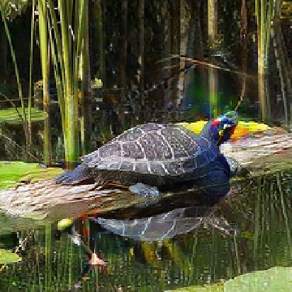
Published as a conference paper at ICLR 2019

   step). Another one is the potential need for more training data as shown recently in (Schmidt et al.,
   2018). These costs make training more demanding, but is that the whole price of being adversarially
   robust? In particular, if we are willing to pay these costs: Are robust classifiers better than standard
   ones in every other aspect? This is the key question that motivates our work.

                                        2-trained                                                  2-trained                                                    2-trained
                        99                                                            90
Standard Accuracy (%)

                                                              Standard Accuracy (%)

                                                                                                                          Standard Accuracy (%)
                                                                                                                                                  90
                        98                                                            80                                                          80

                        97                                                            70                                                          70

                                                    train =                           60                       train =                            60
                        96
                                                        0                                                       0                                 50
                                                                                                                                                                            train =
                                                        0.5                           50                        20/255
                        95                                                                                                                        40
                                                        1.5                           40                        80/255                                                          0
                        94                              2.5                                                     320/255                           30                            0.5
                             103             104                                      30102       103          104                                        103         104        105
                                   # Training Samples                                         # Training Samples                                       # Training Samples
                                    (a) MNIST                                                 (b) CIFAR-10                                         (c) Restricted ImageNet

   Figure 1: Comparison of the standard accuracy of models trained against an `2 -bounded adversary
   as a function of size of the training dataset. We observe that when training with few samples,
   adversarial training has a positive effect on model generalization (especially on MNIST). However,
   as training data increase, the standard accuracy of robust models drops below that of the standard
   model (εtrain = 0). Similar results for `∞ trained networks are shown in Figure 6 of Appendix G.

   Adversarial Training as a Form of Data Augmentation Our point of start is a popular view
   of adversarial training as the “ultimate” form of data augmentation. According to this view, the
   adversarial perturbation set ∆ is seen as the set of invariants that a good model should satisfy
   (regardless of the adversarial robustness considerations). Thus, finding the worst-case δ corresponds
   to augmenting the training data in the “most confusing” and thus also “most helpful” manner. A key
   implication of this view is that adversarial training should be beneficial for the standard accuracy of a
   model (Torkamani & Lowd, 2013; 2014; Goodfellow et al., 2014b; Miyato et al., 2018).
   Indeed, in Figure 1, we see this effect, when classifiers are trained with relatively few samples
   (particularly on MNIST). In this setting, the amount of training data available is insufficient to learn
   a good standard classifier and the set of adversarial perturbations used is “compatible” with the
   learning task. (That is, good standard models for this task need to be also somewhat invariant to these
   perturbations.) In such regime, robust training does indeed act as data augmentation, regularizing the
   model and leading to a better solution (from standard accuracy point of view). (Note that this effect
   seems less pronounced for CIFAR-10, possibly because `p -invariance is not as important for a good
   standard CIFAR-10 classifier.)
   Surprisingly however, in Figure 6 we see that as we include more samples in the training set,
   this positive effect becomes less significant. In fact, after some point adversarial training actually
   decreases the standard accuracy. In Figure 7 in Appendix G we study the behaviour of models trained
   using adversarial training with different `p -bounded adversaries. We observe a steady decline in
   standard accuracy as the strength of the adversary increases. (Note that this still holds if we train on
   batches that also contain natural examples, as in Kurakin et al. (2016a). See Appendix B.) Similar
   effects were also observed in prior work (Kurakin et al., 2016b; Madry et al., 2017; Dvijotham et al.,
   2018b; Wong et al., 2018; Xiao et al., 2018b; Su et al., 2018; Babbar & Schölkopf, 2018).
   The goal of this work is to illustrate and explain the roots of this phenomenon. In particular, we
   would like to understand:

                         Why does there seem to be a trade-off between standard and adversarially robust accuracy?

   As we will show, this effect is not an artifact of our adversarial training methods but in fact is
   inevitable consequence of different goals of adversarial robustness and standard generalization.

                                                                                                        3
Published as a conference paper at ICLR 2019

2.1   A DVERSARIAL ROBUSTNESS MIGHT BE INCOMPATIBLE WITH STANDARD ACCURACY

As we discussed above, we often observe that employing adversarial training leads to a decrease in
a model’s standard accuracy. In what follows, we show that this phenomenon is a manifestation of
an inherent tension between standard accuracy and adversarially robust accuracy. In particular, we
present a theoretical model that demonstrates it. In fact, this phenomenon can be illustrated in a fairly
simple setting which suggests that it is quite prevalent.

Our binary classification task Our data model consists of input-label pairs (x, y) sampled from a
distribution D as follows:

           u.a.r                     +y, w.p. p                              i.i.d
         y ∼ {−1, +1},        x1 =                   ,      x2 , . . . , xd+1 ∼ N (ηy, 1),    (3)
                                     −y, w.p. 1 − p
where N (µ, σ 2 ) is a normal distribution with mean µ and variance σ 2 , and p ≥ 0.5. We chose √  η to
be large enough so that a simple classifier attains high standard accuracy (>99%) – e.g. η = Θ(1/ d)
will suffice. The parameter p quantifies how correlated the feature x1 is with the label. For the sake
of example, we can think of p as being 0.95. This choice is fairly arbitrary; the trade-off between
standard and robust accuracy will be qualitatively similar for any p < 1.

Standard classification is easy Note that samples from D consist of a single feature that is
moderately correlated with the label and d other features that are only very weakly correlated
with it. Despite the fact that each one of the latter type of features individually is hardly predictive of
the correct label, this distribution turns out to be fairly simple to classify from a standard accuracy
perspective. Specifically, a natural (linear) classifier

                                         >                               1       1
                      favg (x) := sign(wunif x), where wunif := 0, , . . . ,         ,                  (4)
                                                                         d       d
achieves standard accuracy arbitrarily close to 100%, for d large enough. Indeed, observe that
                                                  " d                  #
                                                   yX                                  1
  Pr[favg (x) = y] = Pr[sign(wunif x) = y] = Pr          N (ηy, 1) > 0 = Pr N η,           >0 ,
                                                   d i=1                               d
                             √
which is > 99% when η ≥ 3/ d.

Adversarially robust classification Note that in our discussion so far, we effectively viewed the
average of x2 , . . . , xd+1 as a single “meta-feature” that is highly correlated with the correct label. For
a standard classifier, any feature that is even slightly correlated with the label is useful. As a result, a
standard classifier will take advantage (and thus rely on) the weakly correlated features x2 , . . . , xd+1
(by implicitly pooling information) to achieve almost perfect standard accuracy.
However, this analogy breaks completely in the adversarial setting. In particular, an `∞ -bounded
adversary that is only allowed to perturb each feature by a moderate ε can effectively override the
effect of the aforementioned meta-feature. For instance, if ε = 2η, an adversary can shift each weakly-
correlated feature towards −y. The classifier would now see a perturbed input x0 such that each of the
features x02 , . . . , x0d+1 are sampled i.i.d. from N (−ηy, 1) (i.e., now becoming anti-correlated with
the correct label). Thus, when ε ≥ 2η, the adversary can essentially simulate the distribution of the
weakly-correlated features as if belonging to the wrong class.
Formally, the probability of the meta-feature correctly predicting y in this setting (4) is
              min Pr[sign(x + δ) = y] = Pr [N (η, 1) − ε > 0] = Pr [N (−η, 1) > 0] .
            kδk∞ ≤ε

As a result, the simple classifier in (4) that relies solely on these features cannot get adversarial
accuracy better than 1%.
Intriguingly, this discussion draws a distinction between robust features (x1 ) and non-robust features
(x2 , . . . , xd+1 ) that arises in the adversarial setting. While the meta-feature is far more predictive of
the true label, it is extremely unreliable in the presence of an adversary. Hence, a tension between
standard and adversarial accuracy arises. Any classifier that aims for high accuracy (say > 99%) will

                                                     4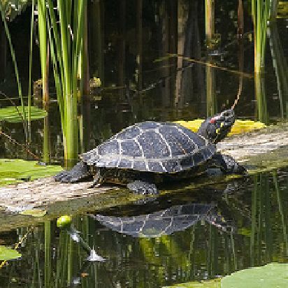
Published as a conference paper at ICLR 2019

have to heavily rely on non-robust features (the robust feature provides only, say, 95% accuracy).
However, since the non-robust features can be arbitrarily manipulated, this classifier will inevitably
have low adversarial accuracy. We make this formal in the following theorem proved in Appendix C.
Theorem 2.1 (Robustness-accuracy trade-off). Any classifier that attains at least 1 − δ standard
                                           p
accuracy on D has robust accuracy at most 1−p δ against an `∞ -bounded adversary with ε ≥ 2η.

This bound implies that if p < 1, as standard accuracy approaches 100% (δ → 0), adversarial
accuracy falls to 0%. As a concrete example, consider p = 0.95, then any classifier with standard
accuracy more than 1 − δ will have robust accuracy at most 19δ 1 . Also it is worth noting that the
theorem is tight. If δ = 1 − p, both the standard and adversarial accuracies are bounded by p which
is attained by the classifier that relies solely on the first feature. Additionally, note that compared to
the scale of the features ±1, the
                                √ value of ε required to manipulate the standard classifier is very small
(ε = O(η), where η = O(1/ d)).

On the (non-)existence of an accurate and robust classifier It might be natural to expect that in
the regime of infinite data, the standard classifier itself acts as a robust classifier. Note however, that
this is not true for the setting we analyze above. Here, the trade-off between standard and adversarial
accuracy is an inherent trait of the data distribution itself and not due to having insufficient samples.
In this particular classification task, we (implicitly) assumed that there does not exist a classifier that
is both robust and very accurate (i.e. > 99% standard and robust accuracy). Thus, for this task, any
classifier that is very accurate (including the Bayes classifier – the classifier minimizing classification
error having full-information about the distribution) will necessarily be non-robust.
This seemingly goes against the common assumption in adversarial ML that humans are such perfect
robust and accurate classifiers for standard datasets. However, note that there is no concrete evidence
supporting this assumption. In fact, humans often have far from perfect performance in vision
benchmarks (Karpathy, 2011; 2014; Russakovsky et al., 2015) and are outperformed by ML models
in certain tasks (He et al., 2015b; Gastaldi, 2017). It is plausible that standard ML models are able to
outperform humans in these tasks by relying on brittle features that humans are naturally invariant to
and the observed decrease in performance might be the manifestation of that.

2.2   T HE IMPORTANCE OF ADVERSARIAL TRAINING

As we have seen in the distributional model D (3), a classifier that achieves very high standard
accuracy (1) will inevitably have near-zero adversarial accuracy. This is true even when a classifier
with reasonable standard and robust accuracy exists. Hence, in an adversarial setting (2), where
the goal is to achieve high adversarial accuracy, the training procedure needs to be modified. We
now make this phenomenon concrete for linear classifiers trained using the soft-margin SVM loss.
Specifically, in Appendix D we prove the following theorem.
                                                           √
Theorem 2.2 (Adversarial training matters). For η ≥ 4/ d and p ≤ 0.975 (the first feature is not
perfect), a soft-margin SVM classifier of unit weight norm minimizing the distributional loss achieves
a standard accuracy of > 99% and adversarial accuracy of < 1% against an `∞ -bounded adversary
of ε ≥ 2η. Minimizing the distributional adversarial loss instead leads to a robust classifier that has
standard and adversarial accuracy of p against any ε < 1.

This theorem shows that if our focus is on robust models, adversarial training is crucial to achieve
non-trivial adversarial accuracy in this setting. Simply optimizing the standard accuracy of the model
(i.e. standard training) leads to poor robust accuracy. Soft-margin SVM classifiers and the constant
0.975 are chosen for mathematical convenience. Our proofs do not depend on them in a crucial way
and can be adapted, in a straightforward manner, to other natural settings, e.g. logistic regression.

Transferability An interesting implication of our analysis is that standard training produces clas-
sifiers that rely on features that are weakly correlated with the correct label. This will be true for
any classifier trained on the same distribution. Hence, the adversarial examples that are created by
perturbing each feature in the direction of −y will transfer across classifiers trained on independent
    1
      Hence, any classifier with standard accuracy ≥ 99% has robust accuracy ≤ 19% and any classifier with
standard accuracy ≥ 96% has robust accuracy ≤ 76%.

                                                    5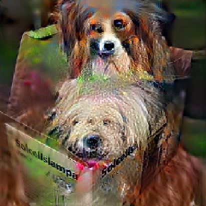
Published as a conference paper at ICLR 2019

             6        2      7                bird    airplane   frog               insect     dog     primate

Original

                                  Original

                                                                        Sample
Standard

                                  Standard

                                                                        Natural
                                  -trained

                                                                        -trained
-trained

                                  2-trained

                                                                        2-trained
2-trained

                 (a) MNIST                       (b) CIFAR-10                       (c) Restricted ImageNet

Figure 2: Visualization of the loss gradient with respect to input pixels. Recall that these gradients
highlight the input features which affect the loss most strongly, and thus are important for the classi-
fier’s prediction. We observe that the gradients are significantly more interpretable for adversarially
trained networks – they align well with perceptually relevant features. In contrast, for standard
networks they appear very noisy. We observe that gradients of `∞ -trained models tend to be sparser
than those of `2 -trained models. (For MNIST, blue and red pixels denote positive and negative
gradient regions respectively. For CIFAR-10 and ImageNet, we clip gradients to within ±3σ and
rescale them to lie in the [0, 1] range.) Additional visualizations are in Figure 10 of Appendix G.

samples from the distribution. This constitutes an interesting manifestation of the generally observed
phenomenon of transferability (Szegedy et al., 2013) and might hint at its origin.

Empirical examination In Section 2.1, we showed that the trade-off between standard accuracy
and robustness might be inevitable. To examine how representative our theoretical model is of
real-world datasets, we also experimentally investigate this issue on MNIST (LeCun et al., 1998)
as it is amenable to linear classifiers. Interestingly, we observe a qualitatively similar behavior. For
instance, in Figure 5(b) in Appendix E, we see that the standard classifier assigns weight to even
weakly-correlated features. (Note that in settings with finite training data, such brittle features could
arise even from noise – see Appendix E.) The robust classifier on the other hand does not assign any
weight beyond a certain threshold. Further, we find that it is possible to obtain a robust classifier
by directly training a standard model using only features that are relatively well-correlated with the
label (without adversarial training). As expected, as more features are incorporated into the training,
the standard accuracy is improved at the cost of robustness (see Appendix E Figure 5(c)).

3           U NEXPECTED BENEFITS OF ADVERSARIAL ROBUSTNESS
In Section 2, we established that robust and standard models might depend on very different sets of
features. We demonstrated how this can lead to a decrease in standard accuracy for robust models. In
this section, we will argue that the features learned by robust models can also be beneficial.
At a high level, robustness to adversarial perturbations can be viewed as an invariance property of
a model. A model that achieves small loss for all perturbations in the set ∆, will necessarily have
learned features that are invariant to such perturbations. Thus, robust training can be viewed as a
method to embed certain invariances in a model. Since we also expect humans to be invariant to these
perturbations (e.g. small `p -bounded changes of the pixels), robust models will be more aligned with
human vision than standard models. In this section, we present evidence supporting the view.

Loss gradients in the input space align well with human perception As a starting point, we
want to investigate which features of the input most strongly affect the prediction of the classifier
both for standard and robust models. To this end, we visualize the gradients of the loss with respect
to individual features (pixels) of the input in Figure 2. We observe that gradients for adversarially

                                                          6
Published as a conference paper at ICLR 2019
Original Standard -trained 2-trained Original Standard -trained 2-trained
4 8 8 8 airplane bird bird bird
9 4 7 7 dog deer bird deer
(a) MNIST (b) CIFAR-10
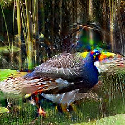
Original Standard -trained 2-trained
primate dog dog dog
bird turtle dog cat
(c) Restricted ImageNet
Figure 3: Visualizing large-ε adversarial examples for standard and robust (`2 /`∞ -adversarial
training) models. We construct these examples by iteratively following the (negative) loss gradient
while staying with `2 -distance of ε from the original image. We observe that the images produced
for robust models effectively capture salient data characteristics and appear similar to examples of a
different class. (The value of ε is equal for all models and much larger than the one used for training.)
Additional examples are visualized in Figure 8 and 9 of Appendix G.
trained networks align well with perceptually relevant features (such as edges) of the input image.
In contrast, for standard networks, these gradients have no coherent patterns and appear very noisy
to humans. We want to emphasize that no preprocessing was applied to the gradients (other than
scaling and clipping for visualization). On the other hand, extraction of interpretable information
from the gradients of standard networks has so far only been possible using additional sophisticated
techniques (Simonyan et al., 2013; Yosinski et al., 2015; Olah et al., 2017).
This observation effectively outlines an approach to train models that align better with human
perception by design. By encoding the correct prior into the set of perturbations ∆, adversarial
training alone might be sufficient to yield interpretable gradients. We believe that this phenomenon
warrants an in-depth investigation and we view our experiments as only exploratory.
Adversarial examples exhibit salient data characteristics Given how the gradients of standard
and robust models are concentrated on qualitatively different input features, we want to investigate
how the adversarial examples of these models appear visually. To find adversarial examples, we
start from a given test image and apply Projected Gradient Descent (PGD; a standard first-order
optimization method) to find the image of highest loss within an `p -ball of radius ε around the original
image 2 . This procedure will change the pixels that are most influential for a particular model’s
predictions and thus hint towards how the model is making its predictions.
The resulting visualizations are presented in Figure 3 (details in Appendix A). Surprisingly, we
can observe that adversarial perturbations for robust models tend to produce salient characteristics
of another class. In fact, the corresponding adversarial examples for robust models can often be
perceived as samples from that class. This behavior is in stark contrast to standard models, for which
adversarial examples appear as noisy variants of the input image.
2
To allow for significant image changes, we will use much larger values of ε than those used during training.
7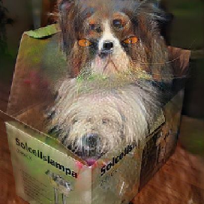
Published as a conference paper at ICLR 2019

These findings provide additional evidence that adversarial training does not necessarily lead to
gradient obfuscation (Athalye et al., 2018). Following the gradient changes the image in a meaningful
way and (eventually) leads to images of different classes. Hence, the robustness of these models does
not stem from having gradients that are ill-suited for first-order methods.

Smooth cross-class interpolations via gradient descent By linearly interpolating between the
original image and the image produced by PGD we can produce a smooth, “perceptually plausible”
interpolation between classes (Figure 4). Such interpolation have thus far been restricted to generative
models such as GANs (Goodfellow et al., 2014a) and VAEs (Kingma & Welling, 2013), involved
manipulation of learned representations (Upchurch et al., 2016), and hand-designed methods (Suwa-
janakorn et al., 2015; Kemelmacher-Shlizerman, 2016). In fact, we conjecture that the similarity of
these inter-class trajectories to GAN interpolations is not a coincidence. We postulate that the saddle
point problem that is key in both these approaches may be at the root of this effect. We hope that
future research will investigate this connection further and explore how to utilize the loss landscape
of robust models as an alternative method to smoothly interpolate between classes.

    Figure 4: Interpolation between original image and large-ε adversarial example as in Figure 3.

4     R ELATED WORK
Due to the large body of related work, we will only focus on the most relevant studies here and
defer the full discussion to Appendix F. Fawzi et al. (2018b) prove upper bounds on the robust of
classifiers and exhibit a standard vs. robust accuracy trade-off for a specific classifier families on a
synthetic task. Their setting also (implicitly) utilizes the notion of robust and non-robust features,
however these features have small magnitude rather than weak correlation. Ross & Doshi-Velez
(2017) propose regularizing the gradient of the classifier with respect to its input. They find that the
resulting classifiers have more interpretable gradients and targeted adversarial examples resemble
the target class for digit and character recognition tasks. There has been recent of work proving
upper bounds on classifier robustness (Gilmer et al., 2018; Schmidt et al., 2018; Fawzi et al., 2018a).
However, this work is orthogonal to ours as in these settings there exist classifiers that are both robust
and accurate.

5     C ONCLUSIONS AND FUTURE DIRECTIONS
In this work, we show that the goal of adversarially robust generalization might fundamentally be at
odds with that of standard generalization. Specifically, we identify an inherent trade-off between the
standard accuracy and adversarial robustness of a model, that provably manifests in a concrete, simple
setting. This trade-off stems from intrinsic differences between the feature learned by standard and
robust models. Our analysis also explains the drop in standard accuracy observed when employing
adversarial training in practice. Moreover, it emphasizes the need to develop robust training methods,
since robustness is unlikely to arise as a consequence of standard training.
We discover that even though adversarial robustness comes at a price, it has some unexpected
benefits. Robust models learn features that align well with salient data characteristics. The root

                                                    8
Published as a conference paper at ICLR 2019

of this phenomenon is that the set of adversarial perturbations encodes some prior for human
perception. Thus, classifiers that are robust to these perturbations are also necessarily invariant to
input modifications that we expect humans to be invariant to. We demonstrate a striking consequence
of this phenomenon: robust models yield clean feature interpolations similar to those obtained from
generative models such as GANs (Goodfellow et al., 2014b). This emphasizes the possibility of a
stronger connection between GANs and adversarial robustness.
Finally, our findings show that the interplay between adversarial robustness and standard classification
might be more nuanced that one might expect. This motivates further work to fully undertand the
relative costs and benefits of each of these notions.

ACKNOWLEDGEMENTS
Shibani Santurkar was supported by the National Science Foundation (NSF) under grants IIS-1447786,
IIS-1607189, and CCF-1563880, and the Intel Corporation. Dimitris Tsipras was supported in part
by the NSF grant CCF-1553428. Aleksander Madry    ˛   was supported in part by an Alfred P. Sloan
Research Fellowship, a Google Research Award, and the NSF grant CCF-1553428.

R EFERENCES
Tensor flow models repository.       https://github.com/tensorflow/models/tree/master/
  resnet, 2017.
Anish Athalye, Logan Engstrom, Andrew Ilyas, and Kevin Kwok. Synthesizing robust adversarial examples.
  arXiv preprint arXiv:1707.07397, 2017.
Anish Athalye, Nicholas Carlini, and David Wagner. Obfuscated gradients give a false sense of security:
  Circumventing defenses to adversarial examples. arXiv preprint arXiv:1802.00420, 2018.
Rohit Babbar and Bernhard Schölkopf.        Adversarial extreme multi-label classification. arXiv preprint
  arXiv:1803.01570, 2018.
Aharon Ben-Tal, Laurent El Ghaoui, and Arkadi Nemirovski. Robust optimization. Princeton University Press,
  2009.
Battista Biggio and Fabio Roli. Wild patterns: Ten years after the rise of adversarial machine learning. arXiv
  preprint arXiv:1712.03141, 2017.
Sébastien Bubeck, Eric Price, and Ilya Razenshteyn. Adversarial examples from computational constraints.
  arXiv preprint arXiv:1805.10204, 2018.
Nicholas Carlini and David Wagner. Towards evaluating the robustness of neural networks. arXiv preprint
  arXiv:1608.04644, 2016.
Nicholas Carlini and David Wagner. Adversarial examples are not easily detected: Bypassing ten detection
  methods. arXiv preprint arXiv:1705.07263, 2017.
Nilesh Dalvi, Pedro Domingos, Mausam, Sumit Sanghai, and Deepak Verma. Adversarial classification. In
  International Conference on Knowledge Discovery and Data Mining (KDD), 2004.
J. Deng, W. Dong, R. Socher, L.-J. Li, K. Li, and L. Fei-Fei. ImageNet: A Large-Scale Hierarchical Image
   Database. In CVPR09, 2009.
Krishnamurthy Dvijotham, Sven Gowal, Robert Stanforth, Relja Arandjelovic, Brendan O’Donoghue,
  Jonathan Uesato, and Pushmeet Kohli. Training verified learners with learned verifiers. arXiv preprint
  arXiv:1805.10265, 2018a.
Krishnamurthy Dvijotham, Robert Stanforth, Sven Gowal, Timothy Mann, and Pushmeet Kohli. A dual approach
  to scalable verification of deep networks. arXiv preprint arXiv:1803.06567, 2018b.
Logan Engstrom, Dimitris Tsipras, Ludwig Schmidt, and Aleksander Madry. A rotation and a translation suffice:
  Fooling cnns with simple transformations. arXiv preprint arXiv:1712.02779, 2017.
Ivan Evtimov, Kevin Eykholt, Earlence Fernandes, Tadayoshi Kohno, Bo Li, Atul Prakash, Amir Rahmati, and
   Dawn Song. Robust physical-world attacks on machine learning models. arXiv preprint arXiv:1707.08945,
   2017.

                                                      9
Published as a conference paper at ICLR 2019

Alhussein Fawzi and Pascal Frossard. Manitest: Are classifiers really invariant? In British Machine Vision
  Conference (BMVC), number EPFL-CONF-210209, 2015.

Alhussein Fawzi, Seyed-Mohsen Moosavi-Dezfooli, and Pascal Frossard. Robustness of classifiers: from
  adversarial to random noise. In Advances in Neural Information Processing Systems, pp. 1632–1640, 2016.

Alhussein Fawzi, Hamza Fawzi, and Omar Fawzi. Adversarial vulnerability for any classifier. arXiv preprint
  arXiv:1802.08686, 2018a.

Alhussein Fawzi, Omar Fawzi, and Pascal Frossard. Analysis of classifiers’ robustness to adversarial perturba-
  tions. Machine Learning, 107(3):481–508, 2018b.

Xavier Gastaldi. Shake-shake regularization. arXiv preprint arXiv:1705.07485, 2017.

Justin Gilmer, Luke Metz, Fartash Faghri, Samuel S Schoenholz, Maithra Raghu, Martin Wattenberg, and Ian
   Goodfellow. Adversarial spheres. arXiv preprint arXiv:1801.02774, 2018.

Ian Goodfellow. Adversarial examples. Presentation at Deep Learning Summer School, 2015. http://
   videolectures.net/deeplearning2015_goodfellow_adversarial_examples/.

Ian Goodfellow, Jean Pouget-Abadie, Mehdi Mirza, Bing Xu, David Warde-Farley, Sherjil Ozair, Aaron
   Courville, and Yoshua Bengio. Generative adversarial nets. In Advances in neural information processing
   systems, pp. 2672–2680, 2014a.

Ian J. Goodfellow, Jonathon Shlens, and Christian Szegedy. Explaining and harnessing adversarial examples.
   arXiv preprint arXiv:1412.6572, 2014b.

Alex Graves, Abdel-rahman Mohamed, and Geoffrey Hinton. Speech recognition with deep recurrent neural
  networks. In Acoustics, speech and signal processing (icassp), 2013 ieee international conference on, pp.
  6645–6649. IEEE, 2013.

Kaiming He, Xiangyu Zhang, Shaoqing Ren, and Jian Sun. Deep residual learning for image recognition. corr
  abs/1512.03385 (2015), 2015a.

Kaiming He, Xiangyu Zhang, Shaoqing Ren, and Jian Sun. Delving deep into rectifiers: Surpassing human-level
  performance on imagenet classification. In Proceedings of the IEEE international conference on computer
  vision, pp. 1026–1034, 2015b.

Andrej Karpathy. Lessons learned from manually classifying cifar-10. http://karpathy.github.io/
  2011/04/27/manually-classifying-cifar10/, 2011. Accessed: 2018-09-23.

Andrej     Karpathy.            What I learned  from   competing against a   Con-
  vNet       on       ImageNet.            http://karpathy.github.io/2014/09/02/
  what-i-learned-from-competing-against-a-convnet-on-imagenet/, 2014.         Ac-
  cessed: 2018-09-23.

Ira Kemelmacher-Shlizerman. Transfiguring portraits. ACM Transactions on Graphics (TOG), 35(4):94, 2016.

Diederik P Kingma and Max Welling. Auto-encoding variational bayes. arXiv preprint arXiv:1312.6114, 2013.

J Zico Kolter and Eric Wong. Provable defenses against adversarial examples via the convex outer adversarial
   polytope. arXiv preprint arXiv:1711.00851, 2017.

Alex Krizhevsky and Geoffrey Hinton. Learning multiple layers of features from tiny images. 2009.

Alex Krizhevsky, Ilya Sutskever, and Geoffrey E Hinton. Imagenet classification with deep convolutional neural
  networks. In Advances in neural information processing systems, pp. 1097–1105, 2012.

Alexey Kurakin, Ian Goodfellow, and Samy Bengio. Adversarial examples in the physical world. arXiv preprint
  arXiv:1607.02533, 2016a.

Alexey Kurakin, Ian J. Goodfellow, and Samy Bengio. Adversarial machine learning at scale. arXiv preprint
  arXiv:1611.01236, 2016b.

Yann LeCun, Corinna Cortes, and Christopher J.C. Burges. The mnist database of handwritten digits. Website,
  1998. URL http://yann.lecun.com/exdb/mnist/.

Yann LeCun, Corinna Cortes, and CJ Burges. Mnist handwritten digit database. AT&T Labs [Online]. Available:
  http://yann. lecun. com/exdb/mnist, 2, 2010.

                                                     10
Published as a conference paper at ICLR 2019
Aleksander Madry, Aleksandar Makelov, Ludwig Schmidt, Dimitris Tsipras, and Adrian Vladu. Towards deep
learning models resistant to adversarial attacks. arXiv preprint arXiv:1706.06083, 2017.
Takeru Miyato, Shin-ichi Maeda, Shin Ishii, and Masanori Koyama. Virtual adversarial training: a regularization
method for supervised and semi-supervised learning. IEEE transactions on pattern analysis and machine
intelligence, 2018.
Volodymyr Mnih, Koray Kavukcuoglu, David Silver, Andrei A Rusu, Joel Veness, Marc G Bellemare, Alex
Graves, Martin Riedmiller, Andreas K Fidjeland, Georg Ostrovski, et al. Human-level control through deep
reinforcement learning. Nature, 518(7540):529, 2015.
Seyed-Mohsen Moosavi-Dezfooli, Alhussein Fawzi, and Pascal Frossard. Deepfool: A simple and accurate
method to fool deep neural networks. In 2016 IEEE Conference on Computer Vision and Pattern Recognition,
CVPR 2016, Las Vegas, NV, USA, June 27-30, 2016, pp. 2574–2582, 2016.
Anh Mai Nguyen, Jason Yosinski, and Jeff Clune. Deep neural networks are easily fooled: High confidence
predictions for unrecognizable images. In IEEE Conference on Computer Vision and Pattern Recognition,
CVPR 2015, Boston, MA, USA, June 7-12, 2015, pp. 427–436, 2015.
Chris Olah, Alexander Mordvintsev, and Ludwig Schubert. Feature visualization. Distill, 2017. doi: 10.23915/
distill.00007. https://distill.pub/2017/feature-visualization.
Aditi Raghunathan, Jacob Steinhardt, and Percy Liang. Certified defenses against adversarial examples. arXiv
preprint arXiv:1801.09344, 2018.
Andrew Slavin Ross and Finale Doshi-Velez. Improving the adversarial robustness and interpretability of deep
neural networks by regularizing their input gradients. arXiv preprint arXiv:1711.09404, 2017.
Olga Russakovsky, Jia Deng, Hao Su, Jonathan Krause, Sanjeev Satheesh, Sean Ma, Zhiheng Huang, Andrej
Karpathy, Aditya Khosla, Michael Bernstein, Alexander C. Berg, and Li Fei-Fei. ImageNet Large Scale
Visual Recognition Challenge. International Journal of Computer Vision (IJCV), 115(3):211–252, 2015. doi:
10.1007/s11263-015-0816-y.
Ludwig Schmidt, Shibani Santurkar, Dimitris Tsipras, Kunal Talwar, and Aleksander Madry.
˛ Adversarially
robust generalization requires more data. arXiv preprint arXiv:1804.11285, 2018.
Mahmood Sharif, Sruti Bhagavatula, Lujo Bauer, and Michael K. Reiter. Accessorize to a crime: Real and
stealthy attacks on state-of-the-art face recognition. In Proceedings of the 2016 ACM SIGSAC Conference on
Computer and Communications Security, Vienna, Austria, October 24-28, 2016, pp. 1528–1540, 2016.
David Silver, Aja Huang, Chris J Maddison, Arthur Guez, Laurent Sifre, George Van Den Driessche, Julian
Schrittwieser, Ioannis Antonoglou, Veda Panneershelvam, Marc Lanctot, et al. Mastering the game of go with
deep neural networks and tree search. nature, 529(7587):484–489, 2016.
Karen Simonyan, Andrea Vedaldi, and Andrew Zisserman. Deep inside convolutional networks: Visualising
image classification models and saliency maps. arXiv preprint arXiv:1312.6034, 2013.
Aman Sinha, Hongseok Namkoong, and John Duchi. Certifiable distributional robustness with principled
adversarial training. arXiv preprint arXiv:1710.10571, 2017.
Dong Su, Huan Zhang, Hongge Chen, Jinfeng Yi, Pin-Yu Chen, and Yupeng Gao. Is robustness the cost of
accuracy?–a comprehensive study on the robustness of 18 deep image classification models. arXiv preprint
arXiv:1808.01688, 2018.
Supasorn Suwajanakorn, Steven M Seitz, and Ira Kemelmacher-Shlizerman. What makes tom hanks look like
tom hanks. In Proceedings of the IEEE International Conference on Computer Vision, pp. 3952–3960, 2015.
Christian Szegedy, Wojciech Zaremba, Ilya Sutskever, Joan Bruna, Dumitru Erhan, Ian J. Goodfellow, and Rob
Fergus. Intriguing properties of neural networks. arXiv preprint arXiv:1312.6199, 2013.
Vincent Tjeng and Russ Tedrake. Verifying neural networks with mixed integer programming. arXiv preprint
arXiv:1711.07356, 2017.
Mohamad Ali Torkamani and Daniel Lowd. On robustness and regularization of structural support vector
machines. In International Conference on Machine Learning, pp. 577–585, 2014.
MohamadAli Torkamani and Daniel Lowd. Convex adversarial collective classification. In International
Conference on Machine Learning, pp. 642–650, 2013.
11Published as a conference paper at ICLR 2019
Jonathan Uesato, Brendan O’Donoghue, Aaron van den Oord, and Pushmeet Kohli. Adversarial risk and the
dangers of evaluating against weak attacks. arXiv preprint arXiv:1802.05666, 2018.
Paul Upchurch, Jacob Gardner, Geoff Pleiss, Robert Pless, Noah Snavely, Kavita Bala, and Kilian Weinberger.
Deep feature interpolation for image content changes. arXiv preprint arXiv:1611.05507, 2016.
Yizhen Wang, Somesh Jha, and Kamalika Chaudhuri. Analyzing the robustness of nearest neighbors to
adversarial examples. arXiv preprint arXiv:1706.03922, 2017.
Eric Wong, Frank Schmidt, Jan Hendrik Metzen, and J Zico Kolter. Scaling provable adversarial defenses. arXiv
preprint arXiv:1805.12514, 2018.
Yuxin Wu et al. Tensorpack. https://github.com/tensorpack/, 2016.
Chaowei Xiao, Jun-Yan Zhu, Bo Li, Warren He, Mingyan Liu, and Dawn Song. Spatially transformed adversarial
examples. arXiv preprint arXiv:1801.02612, 2018a.
Kai Y Xiao, Vincent Tjeng, Nur Muhammad Shafiullah, and Aleksander Madry. Training for faster adversarial
robustness verification via inducing relu stability. arXiv preprint arXiv:1809.03008, 2018b.
Huan Xu and Shie Mannor. Robustness and generalization. Machine learning, 86(3):391–423, 2012.
Jason Yosinski, Jeff Clune, Anh Nguyen, Thomas Fuchs, and Hod Lipson. Understanding neural networks
through deep visualization. arXiv preprint arXiv:1506.06579, 2015.
A E XPERIMENTAL SETUP
A.1 DATASETS
We perform our experimental analysis on the MNIST (LeCun et al., 2010), CIFAR-10 (Krizhevsky
& Hinton, 2009) and (restricted) ImageNet (Deng et al., 2009) datasets. For binary classification,
we filter out all the images from the MNIST dataset other than the “5” and “7” labelled examples.
For the ImageNet dataset, adversarial training is significantly harder since the classification problem
is challenging by itself and standard classifiers are already computationally expensive to train. We
thus restrict our focus to a smaller subset of the dataset. We group together a subset of existing,
semantically similar ImageNet classes into 8 different super-classes, as shown in Table 1. We train
and evaluate only on examples corresponding to these classes.
Table 1: Classes used in the Restricted ImageNet model. The class ranges are inclusive.
Class Corresponding ImageNet Classes
“Dog” 151 to 268
“Cat” 281 to 285
“Frog” 30 to 32
“Turtle” 33 to 37
“Bird” 80 to 100
“Primate” 365 to 382
“Fish” 389 to 397
“Crab” 118 to 121
“Insect” 300 to 319
A.2 M ODELS
• Binary MNIST (Section 2.2): We train a linear classifier with parameters w ∈ R784 , b ∈ R
on the dataset described in Section A.1 (labels −1 and +1 correspond to images labelled as
“5” and “7” respectively). We use the cross-entropy loss and perform 100 epochs of gradient
descent in training.
12Published as a conference paper at ICLR 2019
• MNIST: We use the simple convolution architecture from the TensorFlow tutorial (TFM,
2017) 3 .
• CIFAR-10: We consider a standard ResNet model (He et al., 2015a). It has 4 groups of
residual layers with filter sizes (16, 16, 32, 64) and 5 residual units each 4 .
• Restricted ImageNet: We use a ResNet-50 (He et al., 2015a) architecture using the code from
the tensorpack repository (Wu et al., 2016). We do not modify the model architecture,
and change the training procedure only by changing the number of examples per “epoch”
from 1,280,000 images to 76,800 images.
A.3 A DVERSARIAL TRAINING
We perform adversarial training to train robust classifiers following Madry et al. (2017). Specifically,
we train against a projected gradient descent (PGD) adversary, starting from a random initial per-
turbation of the training data. We consider adversarial perturbations in `p norm where p = {2, ∞}.
Unless otherwise specified, we use the values of ε provided in Table 2 to train/evaluate our models.
Table 2: Value of ε used for adversarial training/evaluation of each dataset and `p -norm.
Adversary Binary MNIST MNIST CIFAR-10 Restricted Imagenet
`∞ 0.2 0.3 4/255 0.005
`2 - 1.5 0.314 1
A.4 A DVERSARIAL EXAMPLES FOR LARGE ε
The images we generated for Figure 3 were allowed a much larger perturbation from the original
sample in order to produce visible changes to the images. These values are listed in Table 3. Since
Table 3: Value of ε used for large-ε adversarial examples of Figure 3.
Adversary MNIST CIFAR-10 Restricted Imagenet
`∞ 0.3 0.125 0.25
`2 4 4.7 40
these levels of perturbations would allow to truly change the class of the image, training against such
strong adversaries would be impossible. Still, we observe that smaller values of ε suffices to ensure
that the models rely on the most robust (and hence interpretable) features.
B M IXING NATURAL AND ADVERSARIAL EXAMPLES IN EACH BATCH
In order to make sure that the standard accuracy drop in Figure 7 is not an artifact of only training on
adversarial examples, we experimented with including unperturbed examples in each training batch,
following the recommendation of (Kurakin et al., 2016a). We found that while this slightly improves
the standard accuracy of the classifier, it decreases it’s robust accuracy by a roughly proportional
amount, see Table 4.
C P ROOF OF T HEOREM 2.1
The main idea of the proof is that an adversary with ε = 2η is able to change the distribution of
features x2 , . . . , xd+1 to reflect a label of −y instead of y by subtracting εy from each variable. Hence
3
https://github.com/MadryLab/mnist_challenge/
4
https://github.com/MadryLab/cifar10_challenge/
13Published as a conference paper at ICLR 2019
Table 4: Standard and robust accuracy corresponding to robust training with half natural and half
adversarial samples. The accuracies correspond to standard, robust and half-half training.
Standard Accuracy Robust Accuracy
Norm ε Standard Half-half Robust Standard Half-half Robust
0 99.31% - - - - -
0.1 99.31% 99.43% 99.36% 29.45% 95.29% 95.05%
`∞
0.2 99.31% 99.22% 98.99% 0.05% 90.79% 92.86%
MNIST
0.3 99.31% 99.17% 97.37% 0.00% 89.51% 89.92%
0 99.31% - - - - -
0.5 99.31% 99.35% 99.41% 94.67% 97.60% 97.70%
`2
1.5 99.31% 99.29% 99.24% 56.42% 87.71% 88.59%
2.5 99.31% 99.12% 97.79% 46.36% 60.27% 63.73%
0 92.20% - - - - -
2/255 92.20% 90.13% 89.64% 0.99% 69.10% 69.92%
`∞ 4/255 92.20% 88.27% 86.54% 0.08% 55.60% 57.79%
CIFAR10
8/255 92.20% 84.72% 79.57% 0.00% 37.56% 41.93%
0 92.20% - - - - -
20/255 92.20% 92.04% 91.77% 45.60% 83.94% 84.70%
`2 80/255 92.20% 88.95% 88.38% 8.80% 67.29% 68.69%
320/255 92.20% 81.74% 75.75% 3.30% 34.45% 39.76%
any information that is used from these features to achieve better standard accuracy can be used by
the adversary to reduce adversarial accuracy. We define G+ to be the distribution of x2 , . . . , xd+1
when y = +1 and G− to be that distribution when y = −1. We will consider the setting where
ε = 2η and fix the adversary that replaces xi by xi − yε for each i ≥ 2. This adversary is able to
change G+ to G− in the adversarial setting and vice-versa.
Consider any classifier f (x) that maps an input x to a class in {−1, +1}. Let us fix the probability
that this classifier predicts class +1 for some fixed value of x1 and distribution of x2 , . . . , xd+1 .
Concretely, we define pij to be the probability of predicting +1 given that the first feature has sign i
and the rest of the features are distributed according to Gj . Formally,
p++ = Pr (f (x) = +1 | x1 = +1),
x2,...,d+1 ∼G+
p+− = Pr (f (x) = +1 | x1 = +1),
x2,...,d+1 ∼G−
p−+ = Pr (f (x) = +1 | x1 = −1),
x2,...,d+1 ∼G+
p−− = Pr (f (x) = +1 | x1 = −1).
x2,...,d+1 ∼G−
Using these definitions, we can express the standard accuracy of the classifier as
Pr(f (x) = y) = Pr(y = +1) (p · p++ + (1 − p) · p−+ )
+ Pr(y = −1) (p · (1 − p−− ) + (1 − p) · (1 − p+− ))
1
= (p · p++ + (1 − p) · p−+ + p · (1 − p−− ) + (1 − p) · (1 − p+− ))
2
1
= (p · (1 + p++ − p−− ) + (1 − p) · (1 + p−+ − p+− ))) .
2
14Published as a conference paper at ICLR 2019
Similarly, we can express the accuracy of this classifier against the adversary that replaces G+ with
G− (and vice-versa) as
Pr(f (xadv ) = y) = Pr(y = +1) (p · p+− + (1 − p) · p−− )
+ Pr(y = −1) (p · (1 − p−+ ) + (1 − p) · (1 − p++ ))
1
= (p · p+− + (1 − p) · p−− + p · (1 − p−+ ) + (1 − p) · (1 − p++ ))
2
1
= (p · (1 + p+− − p−+ ) + (1 − p) · (1 + p−− − p++ ))) .
2
For convenience we will define a = 1 − p++ + p−− and b = 1 − p−+ + p+− . Then we can rewrite
1
standard accuracy : (p(2 − a) + (1 − p)(2 − b))
2
1
= 1 − (pa + (1 − p)b),
2
1
adversarial accuracy : ((1 − p)a + pb).
2
We are assuming that the standard accuracy of the classifier is at least 1 − δ for some small δ. This
implies that
1
1 − (pa + (1 − p)b) ≥ 1 − δ =⇒ pa + (1 − p)b ≤ 2δ.
2
Since pij are probabilities, we can guarantee that a ≥ 0. Moreover, since p ≥ 0.5, we have
p/(1 − p) ≥ 1. We use these to upper bound the adversarial accuracy by
p2
1 1
((1 − p)a + pb) ≤ (1 − p) a + pb
2 2 (1 − p)2
p
= (pa + (1 − p)b)
2(1 − p)
p
≤ δ.
1−p
D P ROOF OF T HEOREM 2.2
We consider the problem of fitting the distribution D of (3) by using a standard soft-margin SVM
classifier. Specifically, this can be formulated as:
1
min E max(0, 1 − yw> x) + λkwk22
(5)
w 2
for some value of λ. We will assume that we tune λ such that the optimal solution w∗ has `2 -norm of
1. This is without much loss of generality since our proofs can be adapted to the general case. We
will refer to the first term of (5) as the margin term and the second term as the regularization term.
First we will argue that, due to symmetry, the optimal solution will assign equal weight to all the
features xi for i = 2, . . . , d + 1.
Lemma D.1. Consider an optimal solution w∗ to the optimization problem (5). Then,
wi∗ = wj∗ ∀ i, j ∈ {2, ..., d + 1}.
Proof. Assume that ∃ i, j ∈ {2, ..., d + 1} such that wi∗ 6= wj∗ . Since the distribution of xi and xj
are identical, we can swap the value of wi and wj , to get an alternative set of parameters ŵ that has
the same loss function value (ŵj = wi , ŵi = wj , ŵk = wk for k 6= i, j).
Moreover, since the margin term of the loss is convex in w, using Jensen’s inequality, we get
that averaging w∗ and ŵ will not increase the value of that margin term. Note, however, that
∗
k w 2+ŵ k2 < kw∗ k2 , hence the regularization loss is strictly smaller for the average point. This
contradicts the optimality of w∗ .
15Published as a conference paper at ICLR 2019
√ equal weight to all xi for k ≥ 2, we can replace these
Since every optimal solution will assign
features by their sum (and divide by d for convenience). We will define
d+1
1 X
z=√ xi ,
d i=2
which, by the properties of the normal distribution, is distributed as
√
z ∼ N (yη d, 1).
By assigning a weight of v to that combined feature the optimal solutions can be parametrized as
w> x = w1 x1 + vz,
where the regularization term of the loss is λ(w12 + v 2 )/2.
√
Recall that our chosen value of η is 4/ d, which implies that the contribution of vz is distributed
normally with mean 4yv and variance v 2 . By the concentration of the normal distribution, the
probability of vz being larger than v is large. We will use this fact to show that the optimal classifier
will assign on v at least as much weight as it assigns on w1 .
Lemma D.2. Consider the optimal solution (w1∗ , v ∗ ) of the problem (5). Then
1
v∗ ≥ √ .
2
√
Proof. Assume for the sake of contradiction that v ∗ < 1/ 2. Then, with probability at least 1 − p,
the first feature predicts the wrong label and without enough weight, the remaining features cannot
compensate for it. Concretely,
E[max(0, 1 − yw> x)] ≥ (1 − p) E max 0, 1 + w1 − N 4v, v 2
1 4 1
≥ (1 − p) E max 0, 1 + √ −N √ ,
2 2 2
> (1 − p) · 0.016.
We will now show that a solution that assigns zero weight on the first feature (v = 1 and w1 = 0),
achieves a better margin loss.
E[max(0, 1 − yw> x)] = E [max (0, 1 − N (4, 1))]
< 0.0004.
Hence, as long as p ≤ 0.975, this solution has a smaller margin loss than the original solution. Since
both solutions have the same norm, the solution that assigns weight only on v is better than the
original solution (w1∗ , v ∗ ), contradicting its optimality.
We have established that the learned classifier will assign more weight to v than w1 . Since z will be
at least y with large probability, we will show that the behavior of the classifier depends entirely on z.
Lemma D.3. The standard accuracy of the soft-margin SVM learned for problem (5) is at least 99%.
Proof. √ w1 x1 + vz where vz ∼ N (4yv, v 2 ) and
By Lemma D.2, the classifier predicts the sign of √
v ≥ 1/ 2. Hence with probability at least 99%, vzy > 1/ 2 ≥ w1 and thus the predicted class is y
(the correct class) independent of x1 .
We can utilize the same argument to show that an adversary that changes the distribution of z has
essentially full control over the classifier prediction.
Lemma D.4. The adversarial accuracy of the soft-margin SVM learned for (5) is at most 1% against
an `∞ -bounded adversary of ε = 2η.
16You can also read