Dalmeida, KM and Masala, GL (2021) Hrv features as viable physiological markers for stress detection using wearable devices. Sensors, 21 (8). ISSN ...
←
→
Page content transcription
If your browser does not render page correctly, please read the page content below
Dalmeida, KM and Masala, GL (2021) Hrv features as viable physiological
markers for stress detection using wearable devices. Sensors, 21 (8). ISSN
1424-8220

Downloaded from: https://e-space.mmu.ac.uk/627719/
Version: Published Version
Publisher: MDPI AG
DOI: https://doi.org/10.3390/s21082873
Usage rights: Creative Commons: Attribution 4.0

Please cite the published version

                                             https://e-space.mmu.ac.uk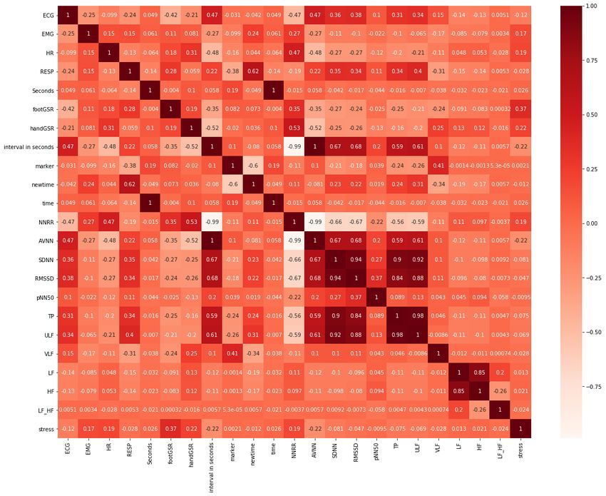
sensors
Article
HRV Features as Viable Physiological Markers for Stress
Detection Using Wearable Devices
Kayisan M. Dalmeida and Giovanni L. Masala *

                                          Department of Computing and Mathematics, Manchester Metropolitan University, Manchester M15 6BH, UK;
                                          kayisan.m.dalmeida@stu.mmu.ac.uk
                                          * Correspondence: g.masala@mmu.ac.uk; Tel.: +44-(0)161-247-1407

                                          Abstract: Stress has been identified as one of the major causes of automobile crashes which then
                                          lead to high rates of fatalities and injuries each year. Stress can be measured via physiological
                                          measurements and in this study the focus will be based on the features that can be extracted by
                                          common wearable devices. Hence, the study will be mainly focusing on heart rate variability (HRV).
                                          This study is aimed at investigating the role of HRV-derived features as stress markers. This is
                                          achieved by developing a good predictive model that can accurately classify stress levels from
                                          ECG-derived HRV features, obtained from automobile drivers, by testing different machine learning
                                          methodologies such as K-Nearest Neighbor (KNN), Support Vector Machines (SVM), Multilayer
                                          Perceptron (MLP), Random Forest (RF) and Gradient Boosting (GB). Moreover, the models obtained
                                          with highest predictive power will be used as reference for the development of a machine learning
                                          model that would be used to classify stress from HRV features derived from heart rate measurements
                                          obtained from wearable devices. We demonstrate that HRV features constitute good markers for stress
                                          detection as the best machine learning model developed achieved a Recall of 80%. Furthermore, this

                                   study indicates that HRV metrics such as the Average of normal-to-normal (NN) intervals (AVNN),
Citation: Dalmeida, K.M.; Masala,         Standard deviation of the average NN intervals (SDNN) and the Root mean square differences
G.L. HRV Features as Viable               of successive NN intervals (RMSSD) were important features for stress detection. The proposed
Physiological Markers for Stress          method can be also used on all applications in which is important to monitor the stress levels in a
Detection Using Wearable Devices.         non-invasive manner, e.g., in physical rehabilitation, anxiety relief or mental wellbeing.
Sensors 2021, 21, 2873. https://
doi.org/10.3390/s21082873                 Keywords: stress; wearable device; machine learning; smart watch; heart rate variability; electrocar-
                                          diogram
Academic Editor: Maria de Fátima
Domingues

Received: 24 March 2021
                                          1. Introduction
Accepted: 14 April 2021
Published: 19 April 2021
                                                Stress can be defined as a biological and psychological response to a combination of
                                          external or internal stressors [1,2], which could be a chemical or biological agent or an
Publisher’s Note: MDPI stays neutral
                                          environmental stimulus that causes stress to an organism [3]. Stress is, in essential, the
with regard to jurisdictional claims in
                                          body’s coping mechanism to any kind of foreign demand or threat. At the molecular level,
published maps and institutional affil-   in a stressful situation the Sympathetic Nervous System (SNS) produces stress hormones,
iations.                                  such as cortisol, which then, via a cascade of events, lead to the increase of available
                                          sources of energy [4]. This large amount of energy is used to fuel a series of physiological
                                          mechanisms such as: increasing the metabolic rate, increasing heart rate and causing the
                                          dilation of blood vessels in the heart and other muscles [5], while decreasing non-essential
Copyright: © 2021 by the authors.
                                          tasks such as immune system and digestion. Once stressors no longer impose a threat to
Licensee MDPI, Basel, Switzerland.
                                          the body, the brain fires up the Parasympathetic Nervous System (PSN) which is in charge
This article is an open access article
                                          of restoring the body to homeostasis. However, if the PSN fails to achieve homeostasis, this
distributed under the terms and           could lead to chronic stress; thus, causing a continual and prolonged activation of the stress
conditions of the Creative Commons        response [6]. Conversely, during acute stress, the stress response develops immediately,
Attribution (CC BY) license (https://     and it is short-lived.
creativecommons.org/licenses/by/                Studies carried out in this field suggest that stress can lead to abnormalities in the
4.0/).                                    cardiac rhythm, and this could lead to arrythmia [7]. Additionally, stress does not only

Sensors 2021, 21, 2873. https://doi.org/10.3390/s21082873                                               https://www.mdpi.com/journal/sensors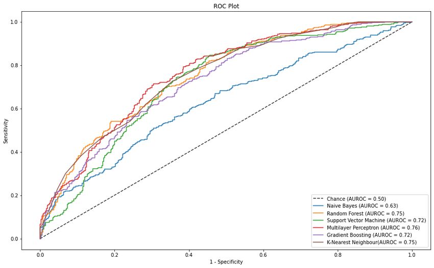
Sensors 2021, 21, 2873                                                                                                2 of 18

                         have physical implications, but it can also be detrimental to one’s mental health; in fact,
                         chronic stress can enhance the chances of developing depression. For these reasons, it is
                         important to develop a system that can detect and measure stress in an individual in a
                         non-invasive manner in such way that stress can be regulated or relieved via personalised
                         medical interventions or even by just alerting the user of their stressful state.
                              Furthermore, stress has been identified as one of the major causes of automobile
                         crashes which then lead to high rates of fatalities and injuries each year [8]. As reported
                         by Virginia Tech Transportation Institute (VTTI) and the National Highway Traffic Safety
                         Administration (NHTSA), lack of attention and stress were the leading cause of traffic
                         accidents in the US, with a rate of ~80%. Therefore, being able to accurately monitor stress
                         in drivers could significantly reduce the amount of road traffic accidents and consequently
                         increase public road safety.
                              Given that stress is regulated by the Autonomous Nervous System, it can be measured
                         via physiological measurements such as Electrocardiogram (ECG), Galvanic Skin Response
                         (GSR), electromyogram (EMG), heart rate variability (HRV), heart rate (HR), blood pressure,
                         breathe frequency, Respiration Rate and Temperature [9]. These are considered to be an
                         accurate methodology for bio signal recording as they cannot be masked or conditioned
                         by human voluntary actions. However, this study will be mainly focusing on HRV, which
                         is controlled by PSN and SNS; therefore, an imbalance in any functions regulated by
                         these two nervous system branches will affect HRV [10]. HRV is the variation in interval
                         between successive normal RR (or NN) intervals [11]; it is derived from an ECG reading
                         and it is measured by calculating the time interval between two consecutive peaks of
                         the heartbeats [12]. As explained in [11] the RR intervals are obtained by calculating the
                         difference between two R waves in the QRS complex.
                              HRV can be subdivided into time domain and frequency domain metrics as described
                         in Table 1.

                         Table 1. Time and Frequency Metrics derived from Heart Rate Variability.

                                                               Time Domain Metrics
                                SDNN            Standard deviation of all NN intervals
                               SDANN            Standard deviation of the average NN intervals
                                AVNN            Average of NN intervals
                                RMSSD           Square root of the mean squared differences of successive RR intervals
                                pNN50           Percentage differences of successive RR intervals larger than 50 ms
                                                            Frequency Domain Metrics
                                  TP            Total Power—total spectral power of all NN intervals up to 0.004 Hz
                                                Low Frequency—total spectral power of all NN intervals with frequency
                                  LF
                                                ranging from 0.04 Hz to 0.15 Hz
                                                High Frequency—total spectral power of all NN intervals with frequency
                                  HF
                                                ranging from 0.15 Hz to 0.4 Hz
                                                Very Low Frequency—total spectral power of all NN intervals with
                                 VLF
                                                frequencies >0.004 Hz
                                                Ultra-Low Frequency—total spectral power of all NN intervals with
                                 ULF
                                                frequencies
Sensors 2021, 21, 2873 3 of 18
a systemic review and meta-analysis on the numerous studies that compared the quality
of HRV measurements acquired from ECG and obtained from portable devices, such as
Elite HRV, Polar H7 and Motorola Droid [13]. Twenty-three studies revealed that HRV
measurements obtained from portable devices resulted in a small amount of absolute error
when compared to ECG; however, this error is acceptable, as this method of acquiring HRV
is more practical and cost-effective, as no laboratory or clinical apparatus are required [13].
Furthermore, the Apple Watch is one of the most best-selling and popular smart-
watches in the market. Studies, carried out by Shcherbina and colleagues [14], demon-
strated that the Apple Watch was the best HR estimating smartwatch with one-minute
granularity and with the lowest overall median error (below 3%) while Samsung Gear S2
reported the highest error. In addition, it is also important to validate the HRV estimation
of the Apple Watch. Currently, the best way to obtain RR raw values from the Apple Watch
is via the Breathe app developed by Apple. Authors in [15] conducted an investigation
that validated the Apple Watch in relation to HRV measurements derived during mental
stress in 20 healthy subjects. In this study, the RR interval series provided by the Apple
watch was validated using the RR interval obtained from Polar H7 [15]. Successively, the
HRV parameters were compared and their ability to identify the Autonomous Nervous
System (ANS) response to mild mental stress was analysed [15]. The results revealed that
the Apple Watch HRV measurements had good reliability and the HRV parameters were
able to indicate changes caused by mild mental stress as it presented a significant decrease
in HF power and RMSSD in stress condition compared to the relax state [15]. Therefore,
this study suggests that the Apple Watch presents a potential non-invasive and reliable
tool for stress monitoring and detection. In this study, raw RR intervals, from beat-to-beat
measurements obtained from the Breathe app, are considered for stress classification.
This study is aimed at developing a good predictive model that can accurately classify
stress levels from ECG-derived HRV features, obtained from automobile drivers, testing
different machine learning methodologies such as K-Nearest Neighbour (KNN), Support
Vector Machines (SVM), Multilayer Perceptron (MLP), Random Forest (RF) and Gradient
Boosting (GB). Moreover, the models obtained with highest predictive power will be used
as a reference for the development of a machine learning model that would be used to
classify stress from HRV features derived from heart rate measurements obtained from
wearable devices in a unsupervised system-based web application.
The paper is organised as follows. Section 2 provides a discussion of related work
conducted in the literature. Section 3 describes the experimental methodology of the study,
including a description of the dataset, pre-processing, hyperparameter tuning and the
design protocol used for the development of a simple stress detection web application
based on Apple Watch derived data. Section 4 presents the experimental results and
Section 5 an intensive discussion of the results obtained. Lastly, Section 6 provides the
concluding remarks of the study, as well as proposed future work.
2. Related Work
As stress level changes so does the HRV and it has been proven that HRV decreases
as stress increases [11]. This is possible because HRV provides a measure to monitor the
activity of the ANS and, therefore, can provide a measure of stress [16]. Authors in [16]
explored the interaction between HRV and mental stress. Here they took ECG recordings
during rest and mental task conditions, which was meant to reflect a stressful state. Linear
HRV measures were then analysed in order to provide information on how the heart
responds to a stressful task. The results demonstrated that the mean RR interval was
significantly lower during a mental task than in the rest condition [16]. This difference
was significant only when time domain parameters (pNN50) and the mean RR interval
were analysed; while the frequency domain measure did not show a significant difference,
although there was an elevated LF/HF in the stressed condition [16]. As LF is associated
with the SNS and HF with PNS, the increased LF/HF ratio does suggest that there is a
higher sympathetic activity in the stress condition compared to the resting state [16].Sensors 2021, 21, 2873 4 of 18
Furthermore, investigations have been carried out in order to accurately classify stress
in drivers via HRV measurements. For example, authors in [17] aimed to classify ECG
data using extracted parameters into highly stressed and normal physiological states of
drivers. In this study, they extracted time domain, frequency domain and nonlinear domain
parameters from HRV obtained by extracting RR intervals from QRS complexes. These
extracted features were fed into the following machine learning classifiers: K Nearest
Neighbor (KNN), radial basis function (RBF) and Support Vector Machine (SVM. The
results showed that SVM with RBF kernel gave the highest results, with 83.33% accuracy,
when applied to time and non-linear parameters, while giving an accuracy of 66.66% with
frequency parameter [17]. This was in concordance with the result obtained by [16] as
the frequency domain parameters did not give a significant difference between rest and
mental tasks.
In this study, instead of analysing how each HRV measure is affected by the onset of
stress, we took into consideration the combination of both time and frequency domain HRV
features and how these aid stress classification with the use of machine learning models.
The performance of the machine learning models was evaluated, taking into consideration
the following metrics: Area Under Receiver Operator Characteristic Curve (AUROC), Re-
call/Sensitivity and F1 score, without relying only on accuracy. Furthermore, we detected
stress in a non-invasive manner using the Apple Watch, from which we extracted heart
rate data, obtained from volunteers subjected to different mental state conditions.
3. Materials and Methods
3.1. Datasets
The first part of this study consists in the development of a good stress predictive
model from ECG-derived HRV measurements. The dataset used was collected at Mas-
sachusetts Institute of Technology (MIT) by Healey and Picard [18], which is freely available
from PhysioNet [19]. The dataset consists of a collection of multi-parameter recordings
obtained from 27 young and healthy individuals while they were driving on a desig-
nated route in the city and highways around Boston, Massachusetts. The driving protocol
involved a route that was planned to put the driver though different levels of stress; specif-
ically, the drive consisted of periods of rest, highway driving and city driving which were
presumed to induce low, medium and high stress, respectively [18]. This investigation
measured four types of physiological signals: ECG, EMG, GSR and respiration. The dataset
is available in the PhysioNet waveform format containing 18 .dat and 18 .hea files with a .txt
metadata file. Each bio-signal .dat file contains the original recording for ECG, EMG, GSR,
HR and Respiration. As the aim of this study is to classify stress based on HRV metrics,
a beat annotation file was created from .dat files by using the WQRS tool that works by
locating QRS complexes in the ECG signal using and gives an annotation file as the out-
put [20]. The annotation file serves the purpose of extracting RR intervals together with its
corresponding timestamp using the PhysioNet HRV toolkit. HRV features were extracted
from the RR intervals by splitting the dataset in windows of 30 s. Time domain features
were calculated using a C implementation that connects Python to the PhysioNet HRV
toolkit and by calling the get_hrv method which returns the HRV metrics. While frequency
domain metrics were obtained by applying the Lomb Periodogram which determines the
power spectrum at any given frequency [21]. GSR signals were used to determine and label
the stress states in drivers, as the marker in the dataset was mainly made of missing values.
The median GSR values were used as the cut-off point, thus, values above the median were
labelled as stress while the values below the median were labelled as no stress. For clarity
reasons, this dataset will be referred to as ‘original-dataset’.
The second portion of this investigation aimed to develop machine learning models
that would classify stress from HRV features derived from HRV measurements obtained
from the Apple Watch. For this purpose, data was collected from 4 Apple Watch users,
who were asked not to exercise or intake caffeine before and on the day of the experiment.
The volunteers were subjected to 2 different conditions. The first condition was a 15-minSensors 2021, 21, 2873 5 of 18
relaxation period where they listened to relaxing lo-fi music. The second was a stressful
condition experienced after an 8-h shift of work. Immediately after each task, the volunteers
were asked to record their beat-to-beat measurements 5 times, using the Apple Breathe App
available on their Apple Watch. The subjects were subjected to these two conditions on
separate days. Thanks to the Breathe App, it was possible to obtain raw RR intervals from
beat-to-beat measurements and all the data was accessible from the user’s Personal Health
Record, which can be exported in XML format via Apple’s Health App. The beat-to-beat
measurements of interests, mapped into the tag, were
extracted from the XML file in Python using xml and pandas modules. Successively, the raw
RR intervals (in seconds) were derived from the beat per minute (bpm) readings using the
following equation:
60
RR = (1)
bpm
Moreover, HRV features were extracted from the calculated RR intervals using the
NumPy library, for time domain, and the pyhrv library, specifically the frequency_domain
module and the Welch’s Method for frequency domain features [22]. This dataset will be
used as a blind test for the obtained classifier, in order to measure its predictive power on
unseen data; hence, this dataset will be referred to as a ‘blind-dataset’ throughout this paper.
The stress prediction of the blind-dataset was performed by a simple web application,
developed using Streamlit. This experimental procedure is illustrated in Figure 1.
Figure 1. Illustration of the experimental procedure followed for stress detection on data obtained from Apple Watch users.
3.1.1. Data Pre-Processing
Firstly, missing values in original-dataset were replaced with the mean value of each
column. Then the data was further split into training and testing datasets with an 80:20
(training:testing) split. From this point onwards, the testing and training data were treated
separately as different entities in order to prevent data overfitting and data leakage. Data
normalisation was done separately on the training and testing set instead of the whole
dataset that could leak information about the test into the train set. Normalisation was
performed using the scikit-learn library, where continuous values are rescaled in a range
between 0 and 1 with the aim of having all numeric columns in the same range, as there
are features that are in different ranges such as ECG, HR, EMG, seconds and HF.separately as different entities in order to prevent data overfitting and data leakage. Data
normalisation was done separately on the training and testing set instead of the whole
dataset that could leak information about the test into the train set. Normalisation was
performed using the scikit-learn library, where continuous values are rescaled in a range
Sensors 2021, 21, 2873 between 0 and 1 with the aim of having all numeric columns in the same range, as there 6 of 18
are features that are in different ranges such as ECG, HR, EMG, seconds and HF.
3.1.2.
3.1.2. Feature
Feature Selection
Selection
Features
Features wereselected
were selected based
based onontheir
theirrelevance
relevancetotothetheclassification
classificationtask
taskthat
thatthis
this
study proposed. This was accomplished using three techniques: Pearson’s
study proposed. This was accomplished using three techniques: Pearson’s Correlation, Correlation,
Recursive
Recursive Feature
Feature Elimination
Elimination (RFE)
(RFE) [23]
[23] and
and Extra
Extra Tree
Tree Classifier
Classifier [24],used
[24], usedtotoestimate
estimate
feature importance. The common least important features from each methoddropped
feature importance. The common least important features from each method were were
from both
dropped fromtraining and testing
both training and datasets; Figure 2Figure
testing datasets; illustrates this process.
2 illustrates this process.
Figure 2. 2.
Figure Flow chart
Flow illustrating
chart thethe
illustrating Feature Selection
Feature Process
Selection implemented
Process inin
implemented this study.
this study.
Pearson’s
Pearson’s Correlation
Correlation calculates
calculates thethe correlation
correlation coefficient
coefficient between
between each
each feature
feature and
and
the
the target
target class
class (stress)
(stress) andand
thisthis
value value
ranges ranges between
between −1 and −11.and
Low1.correlation
Low correlation
is repre- is
represented
sented by values
by values close toclose to 0, with
0, with 0 being0 being no correlation,
no correlation, andand high
high positive
positive andand negative
negative
correlations are achieved with values closer to 1 and −
correlations are achieved with values closer 1 and −1, respectively. In this study,relevant
1, respectively. In this study, rele-
features
vant were
features chosen
were chosenbased
basedon their highly
on their highlypositive
positiveandand highly negative
highly negativecorrelations
correlations with
the target. Feature Importance using Extra Trees Classifier, is
with the target. Feature Importance using Extra Trees Classifier, is an ensemble-based an ensemble-based learning
algorithm
learning that aggregates
algorithm the results
that aggregates of multiple
the results decision
of multiple trees totrees
decision output a classification
to output a clas-
result [24].
sification In each
result [24]. decision, a Gini Importance
In each decision, of the feature
a Gini Importance of theisfeature
calculated which determines
is calculated which
the best feature to split the data on based on the Gini Index mathematical
determines the best feature to split the data on based on the Gini Index mathematical cri- criteria. RFE
functions by recursively eliminating attributes and building the Linear
teria. RFE functions by recursively eliminating attributes and building the Linear Regres- Regression machine
learning
sion machine model on themodel
learning basis ofonthetheselected
basis ofattributes.
the selected It then uses theItaccuracy
attributes. then usesofthe theaccu-
model
that contributes the most to the predictive output of the algorithm.
racy of the model that contributes the most to the predictive output of the algorithm. RFE RFE will then rank each
feature based on importance with 1 being the most important.
will then rank each feature based on importance with 1 being the most important.
AsAsthethe second
second goal
goal ofofthis
thisstudy
studywas wastotodevelop
developa aclassification
classificationmodel
modelthat thatwould
would
classify stress from data obtained from wearable devices, a ‘modified-dataset’
classify stress from data obtained from wearable devices, a ‘modified-dataset’ was created was created
from
from tailoringoriginal-dataset
tailoring original-datasettotopresent
present features
features that
that were
were purely
purelyrelevant
relevanttotothetheattributes
attrib-
calculated from the RR intervals recorded from the device. This also aimed to further
utes calculated from the RR intervals recorded from the device. This also aimed to further
test the classifiers’ performance on a dataset resembling that generated from the wearable
device. Therefore, the relevant features for the modified-dataset were: HR, AVNN, SDNN,
RMSSD, pNN50, TP and VLF. The modified-dataset was also the reference dataset for the
stress detection application which was used to validate the predictive power of the trained
algorithms in a unsupervised system.Sensors 2021, 21, 2873 7 of 18
3.2. Parameter Tuning
In order to achieve the most efficient classification model, hyper-parameter tuning was
performed on each algorithm used in this study to determine the best choice of parameters
that would yield the highest performance. After generating the baseline for each classifier,
where the parameters were set to their default values, a scikit-learn library [25] function
that loops through a set of predefined hyperparameters and fit the model on the training
set was used to perform parameter tuning. Different ranges of each parameter were used
in each grid. The outputs from the grid search are the best parameter combinations that
give the highest predictive performance which were then compared to their corresponding
baseline models. All algorithms in this study were created with the scikit-learn library.
3.2.1. K-Nearest Neighbour
K-Nearest Neighbour (KNN) performs classification based on the closest neighbouring
training points in a given region [26]; thus, the classification of new test data is dependent
on the number of neighbouring labelled examples present at that given location. In order
to obtain the best KNN classification model, different values for k (number of nearest
neighbours) and the p value (the power parameter equivalent to the Euclidean distance
or Manhattan distance) were investigated. The k values investigated ranged from 1 to 30
inclusive, while p values could either be 1 (Manhattan distance) or 2 (Euclidean distance).
The best parameter values resulted from the grid search are as follows: k = 25 and p = 1,
uniform weights was also selected meaning that all points in each neighbourhood are
weighted equally.
3.2.2. Support Vector Machine
The function of the Support Vector Machine (SVM) algorithm is to locate the hyper-
plane in N-dimensional space (where N represents the number of features) that classifies
the data instances into their corresponding class [27] The performance of this algorithm
is affected by hyperparameters such as the soft margin regularization parameter (C) and
kernel, a function that transforms low dimensional inputs space into a higher dimensional
space making the data linearly separable.
For the SVM classification model, different C values (0.001, 0.01, 0.1, 1, 10, 100 and
1000) and kernels, such as Linear kernel, Polynomial (poly) kernel and Gaussian Radial
Basis Function (RBF) kernel were tested. As RBF and poly kernel depends on the gamma
(γ, that determines the distance of influence of a single training point) and degree (the
degree used to find the hyperplane) parameters respectively, 3 grid searches were carried
out for each kernel with γ values of 0.001, 0.01, 0.1, 1, 10, 100 and 1000 and degree values
ranged from 1 to 6 inclusive. The best parameter settings resulted to be RBF kernel with
γ = 10 and C = 100.
3.2.3. Multilayer Perceptron
Multilayer Perceptron (MLP) is a feedforward artificial neural network that was
developed to circumvent the drawbacks and limitations imposed by the single-layer
perceptron [28]. MLPs are made of at least 3 layers of nodes (input layer, hidden layer and
output layer), where each node is connected to every node in the subsequent layer with
a certain weight. MLP’s performance, like other machine learning algorithms, is highly
dependent on hyperparameter tuning of the following parameters: learning rate coefficient
(h), momentum (µ) and the size of the hidden layer. h determines the size of the weight’s
adjustments made at each iteration; h values of 0.3, 0.25, 0.2, 0.15, 0.1, 0.1, 0.005, 0.01 and
0.001 were investigated in the grid search. µ controls the speed of training and learning
rate; this parameter was set to a range between 0 and 1 with intervals of 0.1. Finally, the
size of the hidden layer corresponds to the number of layers and neurones in the hidden
layer; the following hidden layer sizes were analysed (10, 30, 10), (4, 6, 3, 2), (20), (4, 6,
3), (10, 20) and (100, 100, 400), where each value represent the number of neurons at its
corresponding layer position. A configuration of h = 0.001, µ = 0.1 and three hidden layersSensors 2021, 21, 2873 8 of 18
of 100, 10 and 400 nodes, respectively, proved to be the optimal settings for the model
following the grid search.
3.2.4. Random Forest
Random Forest (RF) is an ensemble-based learning algorithm consisting of a combina-
tion of randomly generated decision tree classifiers, the results of which are aggregated
to obtain a better predictive performance [26]. Based on the parameter tuning grid search
performed, the optimal configuration for this algorithm was when the number of trees
in the forest (estimators) was set to 300, out of the values 1, 2, 3, 4, 8, 16, 32, 64 and
100 that were tested, with the maximum number of features set to the square root of the
total number of features, while the log base 2 of the number of features gave a lower
prediction performance.
3.2.5. Gradient Boosting
Gradient Boosting (GB) is also an ensemble-based algorithm composed of multiple
decision trees trained to predict new data and where each tree is dependent on one another.
This model, which is trained in a gradual, sequential and additive manner, is highly
dependent on the learning rate parameter that regulates the shrinkage of the contribution
of each tree to the model. The optimal value for this parameter was found to be 0.14 as
other learning rate values of 1, 0.5, 0.25, 0.1, 0.05 and 0.01 were also tested in the grid search.
A Naïve Bayes probabilistic algorithm [26] was used as the baseline model for perfor-
mance comparison between the other more complex algorithms. The configuration for this
model was kept as simple as possible by utilising the parameters in their default values as
presented by the GuassianNB python model.
Furthermore, in order to determine whether there were statistical differences between
the investigated models and the baseline model, a One-Way ANOVA statistical test with
Tukey’s post Hoc comparison was performed on the mean AUROC scores. The null and
alternate hypothesis formulated were:
Hypothesis 1 (H1). Null Hypothesis: The mean AUROC score for the compared 2 models
are equal.
Hypothesis 2 (H2). Alternative Hypothesis: The mean AUROC score for the 2 compared models
are not equal, at least AUROC value of one model is different from the other.
4. Results
All results, related to original-dataset and modified-dataset, are described in terms
of machine learning metrics such as Area Under Receiver Operator Characteristic Curve
(AUROC), Recall/Sensitivity and F1 score [26], including their standard deviation. Every
machine learning algorithm was run with a five-fold cross validation. Meanwhile, results
from stress classification from data obtained from the Apple Watch are expressed in terms
of prediction probability.
4.1. Feature Selection on Original-Dataset
Feature Selection was performed in order to determine the attributes in the dataset that
most contribute to the classification task. Figure 3 represents the heat map plot obtained
from Pearson’s Correlation. Feature selection scores from RFE, shown in Table 2, indicate
that the most relevant features are those with the lowest score. This also shows that the
best features (score of 1) were time domain HRV metrics such as RMSSD and AVNN, and
frequency domain metrics like TP and ULF, followed by SDNN with a score of 4 (Table 2).
Furthermore, Figure 4 illustrates a histogram of the feature importance scores based on
the Extra Trees Classifier. Figure 4 shows the Gini Importance of each feature, where the
greater the value, the greater the importance of the feature in stress classification.that the best features (score of 1) were time domain HRV metrics such as RMSSD and
AVNN, and frequency domain metrics like TP and ULF, followed by SDNN with a score
of 4 (Table 2). Furthermore, Figure 4 illustrates a histogram of the feature importance
scores based on the Extra Trees Classifier. Figure 4 shows the Gini Importance of each
Sensors 2021, 21, 2873 feature, where the greater the value, the greater the importance of the feature in stress
9 of 18
classification.
Sensors 2021, 21, 2873 10 of 19
Table 2. RFE feature importance score on original-dataset, the most relevant features have the
lowest RFE score.
Feature RFE Score
EMG 1
HR 1
footGSR 1
handGSR 1
Interval in seconds 1
NNRR 1
AVNN 1
RMSSD 1
TP 1
ULF 1
RESP 2
marker 3
SDNN 4
LF_HF 5
LF 6
ECG 7
pNN50 8
HF 9
newtime 10
time 11
VLF 12
Figure
Figure 3. 3. Heatmap
Heat mapplot
plotofofPearson’s
Pearson’s Correlation
Correlation Feature
Feature Selection
Seconds Selectionperformed
performedononoriginal-dataset.
original-dataset.
13
Figure
Figure 4. Feature
4. Feature Importanceof
Importance offeatures
features from
fromoriginal-dataset
original-datasetusing Extra
using Trees
Extra Classifier.
Trees Classifier.Sensors 2021, 21, 2873 10 of 18
Table 2. RFE feature importance score on original-dataset, the most relevant features have the lowest
RFE score.
Feature RFE Score
EMG 1
HR 1
footGSR 1
handGSR 1
Interval in seconds 1
NNRR 1
AVNN 1
RMSSD 1
TP 1
ULF 1
RESP 2
marker 3
SDNN 4
LF_HF 5
LF 6
ECG 7
pNN50 8
HF 9
newtime 10
time 11
VLF 12
Seconds 13
The common features, from each method, that least contributed to classification or
that had the lowest score were dropped from the dataset; these were LF_HF, LF and HF.
Additionally, GSR attributes were also dropped because they presented a very strong
correlation with stress classification as these were used for stress labelling. Thus, in order to
avoid data leakage and overfitting, they were eliminated. Moreover, intuitively redundant
features were also dropped like the time related features marker, due to its high number of
missing values and EMG, given that it is irrelevant in the context of the smart watch.
4.2. Stress Classification on Original-Dataset
In this experiment, stress was classified from bio-signals obtained from subjects who
drove under different stress conditions. The results obtained from hyperparameter tuning,
illustrated in Table 3, showed that the three best models for the classification task imposed
by this dataset were MLP, RF and GB which yielded an AUROC of 83%, 85% and 85%
respectively. Thus, the models have more than 83% probability of correctly classifying
data instances.
Table 3. Comparison of the predictive performance of the best classifiers obtained from the grid
search (trained on original-dataset).
Algorithm AUROC Recall F1 Score
NB 0.60 ± 0.02 0.63 ± 0.04 0.61 ± 0.02
KNN 0.80 ± 0.01 0.76 ± 0.02 0.74 ± 0.01
SVM 0.81 ± 0.01 0.79 ± 0.03 0.77 ± 0.01
MLP 0.83 ± 0.01 0.81 ± 0.07 0.77 ± 0.02
RF 0.85 ± 0.01 0.81 ± 0.03 0.78 ± 0.02
GB 0.85 ± 0.01 0.80 ± 0.02 0.79 ± 0.01
NB, Naïve Bayes; KNN, K Nearest Neighbour; SVM, Support Vector Machine; MLP, Multilayer Perceptron; RF,
Random Forest; GB, Gradient Boosting. NB represent the baseline model used as means of comparison for the
other complex machine learning algorithm.
Moreover, MLP and RF presented a Recall of 81% while GB 80% (Table 3); this indicates
that at least 80% of the predicted Tue Positive instances are actual positives. Therefore, atSensors 2021, 21, 2873 11 of 18
least 80% of the instances predicted to be in the stress class have been correctly classified
as such. Finally, the F1 scores for MLP, RF and GB are 77%, 78% and 79%, respectively;
thus, the model has at least 77% accuracy on the dataset. Figure 3 illustrates the Receiver
Operating Characteristics (ROC) curve for all the classifiers investigated in this study.
Figure 5 consolidates the findings shown in Table 3, illustrating that the models with
the greatest ROC area are GB, RF and MLP. It is also visible that this NB model serves as a
Sensors 2021, 21, 2873 12 of 19
good baseline model as its ROC curve suggest that its classification is nearly due to chance.
A statistical analysis was performed to measure the significance of these results (Table 4).
Figure 5. ROC curve
curve plot
plotof
ofeach
eachclassification
classificationmodel
modeltrained onon
trained original-dataset. The
original-dataset. AUROC
The scores
AUROC were
scores achieved
were by the
achieved by
models
the during
models stress
during prediction
stress of the
prediction of test dataset
the test fromfrom
dataset the original-dataset.
the original-dataset.
Table 4. Statistical
Table 4. Statistical Evaluation
Evaluation of the machine
of the machine learning
learning models.
models.
ModelAA
Model Model
Model B B mean
mean(A)
(A) mean mean(B)
(B) diff diff se
se p-Tukey 1
p-Tukey 1
GB
GB KNN
KNN 0.852
0.852 0.800
0.800 0.0520.052 0.009 0.009 0.001
0.001
GB
GB MLP
MLP 0.8520.852 0.825 0.825 0.027 0.027 0.009
0.009 0.039
0.039
GB
GB NBNB 0.8520.852 0.603 0.603 0.2490.249 0.009
0.009 0.001
0.001
GB
GB RF RF 0.8520.852 0.853 0.853 − 0.001 0.009
−0.001 0.009 0.9
0.9
GB SVM 0.852 0.813 0.039 0.009 0.001
GB SVM 0.852 0.813 0.039 0.009 0.001
KNN MLP 0.800 0.825 −0.025 0.009 0.077
KNN
KNN MLP
NB 0.8000.800 0.603 0.825 0.197 −0.025 0.009
0.009 0.077
0.001
KNN
KNN RFNB 0.8000.800 0.853 0.603 −0.053 0.197 0.009
0.009 0.001
0.001
KNN
KNN SVM RF 0.8000.800 0.813 0.853 −0.013 −0.053 0.009
0.009 0.671
0.001
MLP
KNN NB
SVM 0.8250.800 0.603 0.813 0.222 0.009
−0.013 0.009 0.001
0.671
MLP RF 0.825 0.853 −0.028 0.009 0.036
MLP
MLP SVMNB 0.8250.825 0.813 0.603 0.012 0.222 0.009
0.009
0.001
0.732
MLP
NB RFRF 0.6030.825 0.853 0.853 −0.250 −0.028 0.009
0.009 0.036
0.001
MLP
NB SVM
SVM 0.6030.825 0.813 0.813 −0.210 0.012 0.009
0.009 0.732
0.001
RF
NB SVM RF 0.8530.603 0.813 0.853 0.040−0.250 0.009 0.009 0.001
0.001
1 p values in bold represent statistical significance, where p < 0.05.
NB SVM 0.603 0.813 −0.210 0.009 0.001
RF SVM 0.853 0.813 0.040 0.009 0.001
Table
1 p values in 4bold
shows that there
represent was significance,
statistical a statistical difference between the AUROC means of all
where p < 0.05.
hyperparameter-tuned models and the baseline (NB–AUROC = 60%) as the p < 0.05. This
confirms
Tablethat the parameter
4 shows that theretuning did improve
was a statistical the model’s
difference performance
between significantly,
the AUROC means of
all hyperparameter-tuned models and the baseline (NB–AUROC = 60%) as the p < 0.05.
This confirms that the parameter tuning did improve the model’s performance signifi-
cantly, and thus, H1 is accepted. Moreover, the Tukey’s comparison test showed that there
is a statistically significant difference between the AUROC values of GB and MLP and
between MLP and RF (p < 0.05). However, the differences between GB and RF are notSensors 2021, 21, 2873 12 of 18
and thus, H1 is accepted. Moreover, the Tukey’s comparison test showed that there is a
statistically significant difference between the AUROC values of GB and MLP and between
MLP and RF (p < 0.05). However, the differences between GB and RF are not statistically
significant (p = 0.9). Figure 6 summarises the results obtained during this experimental
Sensors 2021, 21, 2873 series, by illustrating the performance comparison between the hyperparameter-tuned13 of 19
models and the baseline NB model.
Figure6.6.Model
Figure Modelperformance
performancecomparison
comparisonofof machine
machine learning
learning algorithms
algorithms trained
trained on on original-da-
original-dataset.
taset.
4.3. Stress Classification on Modified-Dataset
4.3. Stress
The otherClassification
objectiveonofModified-Dataset
this study was to develop a classification model that would
classify
The stress
otherfrom HRV data
objective obtained
of this fromto
study was wearable
developdevices. To achieve
a classification this,that
model classifiers
would
from Table
classify 3 were
stress used
from HRVfor data
stressobtained
classification
fromof a modified-dataset,
wearable devices. Towhich is athis,
achieve modification
classifiers
of the original-dataset
from Table 3 were used but for
with features
stress that mimicofthose
classification obtained from the
a modified-dataset, wearable
which device.
is a modifi-
Table 5 shows the results obtained during the classification task.
cation of the original-dataset but with features that mimic those obtained from the wear-
able device. Table 5 shows the results obtained during the classification task.
Table 5. Predictive performance of machine learning classifiers on modified-dataset.
Table 5. Predictive performance of machine learning classifiers on modified-dataset.
Algorithm AUROC Recall F1 Score
Algorithm
NB AUROC
0.60 ± 0.02 0.69Recall
± 0.04 F1 ±
0.63 Score
0.02
NB
KNN 0.60
0.74 ± ±0.02
0.02 0.69±±0.02
0.76 0.04 0.63±±0.02
0.71 0.02
SVM
KNN 0.74 ± 0.01
0.74 ± 0.02 0.79 ± 0.02
0.76 ± 0.02 0.74 ± 0.01
0.71 ± 0.02
MLP 0.75 ± 0.01 0.80 ± 0.06 0.72 ± 0.02
SVM 0.74 ± 0.01 0.79 ± 0.02 0.74 ± 0.01
RF 0.77 ± 0.01 0.74 ± 0.01 0.72 ± 0.01
MLP
GB 0.75
0.73 ± ±0.01
0.01 0.80±±0.02
0.70 0.06 0.72±±0.01
0.70 0.02
RF 0.77 ± 0.01 0.74 ± 0.01 0.72 ± 0.01
GB 0.73± 0.01 0.70 ± 0.02 0.70 ± 0.01
As shown in Table 5, MLP seems to be the overall best performing classifier with 75%
AUROC, 80% Recall and 72% F1 score.
As shown in Table 5, MLP seems to be the overall best performing classifier with 75%
In addition, Figure 7 illustrates the Receiver Operating Characteristics (ROC) curve
AUROC, 80% Recall and 72% F1 score.
for all the classifiers used for the classification of modified-dataset.
In addition, Figure 7 illustrates the Receiver Operating Characteristics (ROC) curve
for all the classifiers used for the classification of modified-dataset.Sensors 2021, 21, 2873 14 of 19
Sensors 2021, 21, 2873 13 of 18
Figure7.7.ROC
Figure ROCcurve
curveplot
plotofofeach
eachclassification
classification model
model tested
tested onon modified-dataset.
modified-dataset. TheThe AUROC
AUROC scores
scores
were were achieved
achieved by the models
by the models duringprediction
during stress stress prediction of dataset
of the test the test from
dataset
thefrom the modified-
modified-dataset.
dataset.
Figure 7 shows that the ROC curve from the MLP classifiers seems to be the furthest
awayFigure
from the7 shows
chancethat theand
curve ROC tocurve
have thefrom the MLP
largest areaclassifiers
under theseems
curve.to be the furthest
away from the chance
Additionally, curve and
a statistical to have
analysis the largest
(One-Way area under
ANOVA the test
statistical curve.
with Tukey’s post
Additionally,
Hoc) of the top threeabest statistical analysis
performing (One-Way
algorithms, ANOVA
obtained statistical
from test with Tukey’s
the original-dataset, and
post Hoc)
their of the top three
corresponding best performing
algorithms, from the algorithms, obtained
modified-dataset, was from the original-dataset,
performed in order to
and their corresponding
determine their statistical algorithms, from the modified-dataset,
difference. Moreover, was performed
these results provided additional in order
insight
into which model
to determine would
their be bestdifference.
statistical suited to be implemented
Moreover, inresults
these the stress detection
provided application.
additional in-
As shown
sight intoin Tablemodel
which 6, it is evident
would be that thesuited
best machine to learning algorithms
be implemented in trained on detection
the stress original-
dataset are statistically
application. As shown in theTable
better
6, performing models
it is evident that (p < 0.05),learning
the machine which is expected due
algorithms to
trained
the
on fact that more information
original-dataset on thethe
are statistically dataset
betterisperforming
being fed tomodels
the model(pSensors 2021, 21, 2873 15 of 19
Furthermore, Table 6 indicates that there is no significant difference in the AUROC
Sensors 2021, 21, 2873 values between RF2 and MLP2 (p = 0.31). MLP2 was then chosen as the model that will 14 ofbe
18
implemented in the stress detection web application due to its 80% recall score and overall
performance. Additionally, another One-Way ANOVA statistical test with Tukey’s post
Hoc comparison
Hoc comparison was was performed
performed toto determine
determine whether
whether there
there were
were statistical
statistical differences
differences
between the models
between modelsand andthe
theNaïve
NaïveBayes baseline
Bayes model.
baseline TheThe
model. results determined
results that there
determined that
was awas
there statistical difference
a statistical between
difference the AUROC
between meansmeans
the AUROC of theof
models and the
the models andbaseline
the base-as
the pas=the
line 0.001
p =(results not shown).
0.001 (results not shown).
4.4. Stress
4.4. Stress Classification
Classification from
from HRV
HRV Measurements
Measurements Obtained
Obtained from
from Apple
Apple Watch
Watch
A simple
A simplewebwebapplication
applicationthat
that would
would perform
perform stress
stress classification
classification on HRV
on HRV datadata
up-
uploaded by the user (blind-dataset) was developed with the aim to analyse data
loaded by the user (blind-dataset) was developed with the aim to analyse data extracted extracted
using wearable devices. The aim of this process was to test the predictive power of the
using wearable devices. The aim of this process was to test the predictive power of the
chosen model on data obtained from real participants. The application was developed in
chosen model on data obtained from real participants. The application was developed in
Python using the Streamlit framework and it is programmed in such way that the user can
Python using the Streamlit framework and it is programmed in such way that the user can
upload a csv format data, which will be first normalised and then classified as “stress” or
upload a csv format data, which will be first normalised and then classified as “stress” or
“no stress” using the saved MLP model with Recall 80% and AUROC of 75%. Firstly, the
“no stress” using the saved MLP model with Recall 80% and AUROC of 75%. Firstly, the
application will prompt the user to insert the csv file in the side menu bar. Secondly, the
application will prompt the user to insert the csv file in the side menu bar. Secondly, the
backend code will normalise the input data, so all data instances are within the same range,
backend code will normalise the input data, so all data instances are within the same
and display the inserted and normalised data in a tabular format. Thirdly, the normalised
range, and display the inserted and normalised data in a tabular format. Thirdly, the nor-
data undergoes classification, and the results are displayed as Prediction Probability, shown
malised data undergoes classification, and the results are displayed as Prediction Proba-
in Figure 8.
bility, shown in Figure 8.
Figure 8. User Interface of the Stress Detection Web Application developed using Streamlit.
Figure 8. User Interface of the Stress Detection Web Application developed using Streamlit.
After running the program with the input data derived from the volunteers, the pre-
diction probabilities for the model to predict an instance as stress or no stress were recorded
for the different stress scenarios. Figure 9 summarises the results of this investigation in a
bar chart presenting the mean prediction probabilities.After running the program with the input data derived from the volunteers, the pre-
diction probabilities for the model to predict an instance as stress or no stress were rec-
Sensors 2021, 21, 2873 orded for the different stress scenarios. Figure 9 summarises the results of this investiga-
15 of 18
tion in a bar chart presenting the mean prediction probabilities.
Figure 9.
Figure 9. Mean
Mean Prediction
PredictionProbability
Probabilityobtain
obtainfrom
fromthe
thestress
stressdetection
detectionapp
appwith
withvolunteers
volunteersinput
input
data, who were subjected to different stress conditions (after work stress and relaxation).
data, who were subjected to different stress conditions (after work stress and relaxation).
As displayed in
in Figure
Figure 9,
9, the
themodel
modelwas
wasable
abletotocorrectly
correctlyclassify
classifyaastress
stressstate
statewith
witha
aprediction
predictionprobability of of
probability 71 71
± 0.1%. Additionally,
± 0.1%. it was
Additionally, it able
was to achieve
able a prediction
to achieve prob-
a prediction
ability of 79of
probability ± 0.3% whenwhen
79 ± 0.3% the model was presented
the model with with
was presented a relaxing situation.
a relaxing situation.
5. Discussion
Stress has been identified
identified as one of the major causes of automobile
automobile crashes
crashes [8][8] and
and an
an
important player in
important player in the
thedevelopment
developmentofofcardiac
cardiacarrythmia
arrythmia[7];[7];therefore,
therefore, it it
is is important
important to
to
be be able
able to detect
to detect andand measure
measure stressstress in a non-invasive
in a non-invasive and efficient
and efficient manner. manner.
In thisIn this
study,
study, to accomplish
to accomplish this, wethis, we address
address the stressthedetection
stress detection
problemproblem
by usingby using traditional
traditional machine
machine learning algorithms which were trained on ECG-derived
learning algorithms which were trained on ECG-derived HRV metrics obtained HRV metrics obtained
from au-
from automobile
tomobile drivers [18,19].
drivers [18,19].
In
In this paper, stress
this paper, classification was
stress classification performed mainly
was performed mainly using
using HRV-derived
HRV-derived featuresfeatures
as
as studies have shown that HRV is impacted during changes in stress levels, given that
studies have shown that HRV is impacted during changes in stress levels, given that it
it
is highly controlled by the ANS [10]. Moreover, other investigations proved
is highly controlled by the ANS [10]. Moreover, other investigations proved that RMSSD, that RMSSD,
AVNN
AVNNand andSDNN
SDNNwere wereevaluated
evaluatedasasbeing
beingthe
themost
mostreliable HRV
reliable HRV metrics
metrics in in
distinguishing
distinguish-
between stressful and non-stressful situations [28]. Those findings
ing between stressful and non-stressful situations [28]. Those findings were were also confirmed in
also con-
this study as shown in Table 2, where AVNN, RMSSD and SDNN were
firmed in this study as shown in Table 2, where AVNN, RMSSD and SDNN were classi- classified as the HRV
features with the highest RFE feature importance scores. Therefore, they were considered
fied as the HRV features with the highest RFE feature importance scores. Therefore, they
to be the features that contribute the most in the stress classification performance of the
were considered to be the features that contribute the most in the stress classification per-
model. This further confirms that HRV features are viable markers for stress detection.
formance of the model. This further confirms that HRV features are viable markers for
Following hyperparameter tuning, we were able to produce stress classification mod-
stress detection.
els with high predictive power. As shown in Table 3, the best 3 models for the classification
Following hyperparameter tuning, we were able to produce stress classification mod-
task imposed by original-dataset were MLP, RF and GB with AUROC of 83%, 85% and 85%,
els with high predictive power. As shown in Table 3, the best 3 models for the classifica-
respectively; thus, these classifiers have ~84% probability of successfully distinguishing
tion task imposed by original-dataset were MLP, RF and GB with AUROC of 83%, 85%
between the stress and no stress class. In addition, MLP and RF gave Recall scores of
and 85%, respectively; thus, these classifiers have ~84% probability of successfully distin-
81% while GB of 80%; indicating that ~80% of the predicted positive instances are actual
guishing between the stress and no stress class. In addition, MLP and RF gave Recall
positives. Furthermore, these scores were statistically greater than the Naïve Bayes baseline
scores of 81% while GB of 80%; indicating that ~80% of the predicted positive instances
model (p < 0.05) as illustrated in Table 4.
There are very few studies performed on stress classification in drivers using HRV
derived features [17,18], although each study took a different approach to the classification
problem, the classification yielded similar results. For instance, [17] investigated KNN,
SVM-RBF and Linear SVM as their potential classifiers for stress detection. Their resultsSensors 2021, 21, 2873 16 of 18
suggested that SVM with RBF kernel was the best performing model by giving an accuracy
of 83% [17]. However, more extensive investigation is necessary to corroborate this finding
by also considering other classification metrics.
It is also imperative to discuss the fact that stress is a result of a combination of external
(environment) and internal factors (e.g., mental health). Thus, stress could be perceived
as a subjective mental state; for example, certain situations like a drive in the city or in
the highway might not induce the same level of stress in every individual. For instance,
individuals suffering from anxiety could feel stressed in such conditions. Additionally,
stress could be induced from the invasive apparatus used such as the electrodes placed in
different parts of their body and the sensor placed around their diaphragm in [18]; the fact
that the subject is aware that they are being monitored for changes in their mental state
could also impact their stress levels. For this reason, is important to use less intrusive and
everyday devices such as smart watches or mobile phones that are already an essential
part of life in this modern society.
In this paper we also aimed to develop a classification model that would detect stress
from data obtained from the Apple Watch. For this purpose, the best classifiers trained on
original-dataset were tested for the classification of the modified-dataset which presented
features that mimic those derived from the wearable device. Table 5 demonstrates that the
overall ideal model for the stress classification of HRV features derived from wearable-
obtained RR intervals, is MLP with a AUROC of 75% and a Recall of 80%. This was
determined based on the Recall score, as in this stress classification task there is a high cost
associated with False Negatives. For instance, if an individual’s condition, which is actually
stressed, is predicted as not stressed, the cost associated with this False Negative can be
high, especially in a medical or driving context which could then lead to a misdiagnosis
or a car accident respectively. Therefore, it is imperative to select the model with the
highest sensitivity.
Figure 8 shows the user interface (UI) of the simple stress detection web application.
The purpose of this was simply to provide a visual UI to demonstrate the software func-
tionality. This could then be implemented into a mobile or car application where the user
would be alerted when stress is detected and would prompt them to relax or take breaks.
The blind-dataset, obtained from the volunteers, served as a blind test for the MLP
classifier in order to measure its predictive power on unseen data in an unsupervised
application system.
When classifying a stressful task, the web application was able to correctly predict
stress conditions with a 71% prediction probability. Additionally, it was able to achieve
a prediction probability of 79% when the model was presented with a relaxing state.
However, it is important to further improve the model’s performance by investigating
multiple stress levels in order to obtain more accurate stress detection.
6. Conclusions
In this paper, we developed a comparative study to determine the viability of HRV
features as physiological markers for stress detection. This was achieved by computing
different supervised machine learning models to determine which model can be used to
analyse data extracted using wearable devices. The MLP model was considered to be an
ideal algorithm for stress classification due to its 80% sensitivity score. The predictive
power of this classifier was found to be statistically greater compared to the baseline model
created with the Naïve Bayes algorithm with a p value of 0.001. This model was then
implemented in the unsupervised stress detection application where stress can be detected
from blind dataset of HRV features, and extracted from real users using wearable devices
under different stress conditions.
A benefit of this study is that there is a need for technologies that would monitor
stress in drivers in order to reduce car crashes, as nearly 80% of road incidents are due to
drivers being under stress. This project could be the initial steps for tackling this problem.
In fact, the algorithm produced in this model could be implemented in smart cars. So,You can also read