On Segmented Predistortion for Linearization of RF Power Amplifiers
←
→
Page content transcription
If your browser does not render page correctly, please read the page content below
RADIOENGINEERING, VOL. 29, NO. 1, APRIL 2020                                                                                         21

                          On Segmented Predistortion
                    for Linearization of RF Power Amplifiers
                                                      Genevieve BAUDOIN

            ESYCOM, UMR CNRS 9007, Gustave Eiffel University, ESIEE Paris, 93162 Noisy-le-Grand, France

                                                     genevieve.baudoin@esiee.fr

                                          Submitted February 6, 2020 / Accepted February 28, 2020

Abstract. This paper presents a general survey of digital               able to pre-compensate for nonlinear distortion and dynamic
predistortion (DPD) techniques with segmentation. A com-                behavior (memory effects) of the PA. Many models of nonlin-
parison of global DPD with two segmented approaches                     ear dynamic system have been proposed for the DPD [1], [2].
namely Vector-Switched DPD and Decomposed Vector Rota-                  They are discrete-time baseband models with complex input
tion DPD is presented with the support of experimentation on            and output signals. Most of them are derived from trun-
a strongly non-linear 3 ways Doherty PA. It shows the interest          cated Volterra series (Memory Polynomial models (MP) [3],
of both segmented approaches in terms of linearization per-             Generalized Memory Polynomial models (GMP) [4], [5])
formance, complexity and ease of implementation compared                or dynamic Volterra series (Dynamic Deviation Reduction-
to the global DPD. The paper starts with some mathemati-                Based models (DDR) [6]) with limitation to finite memory
cal generalities on interpolation and splines. It focuses on            lengths and nonlinearity orders. Neural networks are also
segmented models derived from Volterra series even if the               potential candidates but they require nonlinear optimization
presented principles can also be applied to neural networks.            techniques to update their coefficients which is not very ap-
                                                                        propriate for real-time adaptive DPD.
                                                                              Volterra series present two interesting properties for the
                                                                        modeling of nonlinear dynamic systems: generality and lin-
Keywords                                                                earity of the model in function of their coefficients which
     Digital predistortion, piecewise models, splines, vector-          simplifies their identification. But their number of coeffi-
     switched DPD, decomposed vector rotation DPD, power                cients increases dramatically with memory depth and order
     amplifiers                                                         of nonlinearity. Moreover they are generally built with non-
                                                                        orthogonal basis based on monomials which leads to bad
                                                                        numerical properties for their identification especially for
                                                                        high-order nonlinearity.
1. Introduction                                                               Models derived from Volterra series such as GMP or
                                                                        DDR have proven their effectiveness for numerous applica-
      Digital predistortion is an efficient technique to linearize
                                                                        tions using mildly nonlinear PA such as class AB PA. But
power amplifiers (PA) in wireless transmitters. It is widely
                                                                        advanced architectures of power transmitters with good ef-
used in base stations of cellular communication and broadcast
                                                                        ficiency such as Doherty PA, envelop tracking, switched or
systems. Power amplifiers are critical elements of radiocom-
                                                                        out-phasing PA exhibit strongly nonlinear dynamic behavior
munication systems because their power efficiency conditions
                                                                        more difficult to model. Also, new communication systems
the autonomy and cost of equipments and their linearity in-
                                                                        allow for very high data rate by using very wide bandwidth
fluences communication performance. New waveforms pro-
                                                                        multidimensional signals (e.g. 4G and 5G systems with car-
posed in order to improve spectral occupancy exhibit very
                                                                        rier aggregation and MIMO). It represents new challenges for
high crest factors and are very sensitive to PA nonlinearities.
                                                                        DPD in terms of bandwidth, nonlinearity and dynamic behav-
But to achieve a good power efficiency, it is necessary to op-
                                                                        ior. It becomes difficult for a global DPD model to achieve
erate the PA in a nonlinear region. Linearization techniques
                                                                        an accurate representation of the system with good numeri-
are therefore necessary to limit in-band signal distortion and
                                                                        cal properties and low computational complexity. This has
out of band spectral regrowth.
                                                                        moved research interest towards different local modeling ap-
     The principle of digital predistortion consists in pro-            proaches in which the global operating space is split into
cessing the baseband complex envelop of the PA input signal             several subspaces represented by local models well suited to
by a predistorter (DPD) so that the cascade of the DPD and              each sub-space. These local models have to be joined in some
PA becomes linear up to a certain amplitude value. the DPD              way to cover the global space. One of the motivations is to
should have inverse characteristics of those of the PA to be            decompose a complicated problem into several simpler ones.

DOI: 10.13164/re.2020.0021                                                                                         FEATURE ARTICLE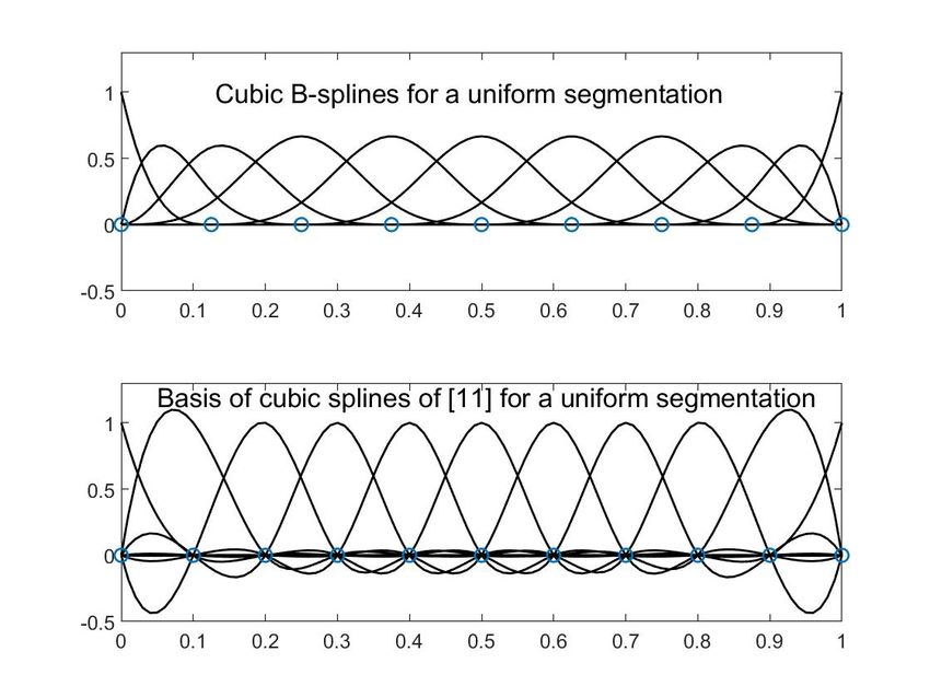
22                                    G. BAUDOIN, ON SEGMENTED PREDISTORTION FOR LINEARIZATION OF RF POWER AMPLIFIERS

Another one is to use the locality to obtain quasi-orthogonal                  can be written using the basis made of Lagrange polynomi-
basis. The decomposition (segmentation) can be applied on                      als L N ,i (x), as:
temporal signal magnitude and phase, on signal spectrum,
                                                                                                                  N
on the system. This segmented or piecewise DPD approach                                                           Õ
                                                                                                   L N f (x) =          f (xi )L N ,i (x),
raises different questions such as:
                                                                                                                  i=0
     • how to partition the original space,                                    with                         Ö x − xj
     • how to determine good models for the different seg-                                   L N ,i (x) =              , i = 0, 1, · · · , N.
                                                                                                                x − xj
                                                                                                            j,i i
       ments of the partition,

     • how to handle DPD operators with complex inputs,                              The approximation error is e(x) = f (x) − p(x) and for
                                                                               f (x) (N + 1) times differentiable:
     • how to handle the dynamic aspects,
                                                                                   ∀x ∈ [a, b] ∃ξ ∈ (min(xi , x), max(xi , x)),
     • how to estimate the coefficients of these local models                                                                                f N +1 (ξ)
       and how to represent them with sparsity,                                    e(x) = f (x) − p(x) = (x − x0 ) · · · (x − x N )                     ,
                                                                                                                                             (N + 1)!
     • how to join the local models.                                                                    (b − a) N +1
                                                                                       max |e(x)| ≤                  max | f N +1 (x)|.
      Piecewise approximation is not a new idea. There has                            x ∈[a,b]           (N + 1)! x ∈[a,b]
been a lot of works in particular on piecewise interpolation or
approximation of nonlinear real-valued functions, e.g. using                        Weierstrass has shown that f can be uniformely ap-
splines. The application of these theories to the case of DPD                  proximated by a polynomial but this is not the interpolation
is not straightforward because of two main reasons:                            polynomial. Indeed, even if the interval between points xi is
                                                                               reduced and the degree of p(x) is increased, p(x) does not
     • the DPD is not a simple function. It is a dynamic non-                  converge towards f (x). This is called Runge’s phenomena.
       linear system;
                                                                                      The approximation error depends on the product v(x) =
     • the input and output of the DPD are complex signals.                    (x−x0 ) · · · (x−x N ) whose value is related to the segmentation
       The DPD is a complex-valued operator of multiple com-                   points x0, x1, · · · , x N . Tchebychev has studied the segmen-
       plex variables.                                                         tation that minimizes the maximum of |v(x)| on the interval
                                                                               [a, b]. Tchebychev’s alternance theorem states that the monic
      This paper presents a general survey of DPD techniques
                                                                               polynomial u(x) of degree n that minimizes L = max |u(x)|
with segmentation in the temporal domain. It also presents
                                                                               (on a given interval) takes alternatively the values ±L, n + 1
an experimental comparison of different approaches. It fo-
                                                                               times. The best solution is u(x) = 2−nTn (x) where Tn is the
cuses on segmented models derived from Volterra series even
                                                                               Tchebychev polynomial of degree n. On the interval [−1, +1],
if the presented principles can also be applied to neural net-
                                                                               it is defined by:
works. It starts with some mathematical generalities on in-
terpolation, approximation and splines (Sec. 2). In Sec. 3 it                         Tn (x) = cos(nφ) with x = cos(φ) for x ∈ [−1, +1].
gives some generalities on modeling and training of DPD.
Section 4 focuses on segmented DPD with functions of a sin-                    The polynomial Tn (x) has n roots xk , Tn (xk ) = 0.
gle real-valued variable. Section 5 is dedicated to segmented                        We can deduce that the segmentation x0, x1, · · · , x N that
DPD that can manage nonlinearity and memory domains.                           minimizes the maximum of |(x − x0 ) · · · (x − x N )| on the in-
Section 6 briefly presents some advanced segmented mul-                        terval [−1, +1] corresponds to the roots of the Tchebychev’s
tidimensional DPD for multiband or MIMO applications.                          polynomial of degree N + 1. They are given by:
Section 7 is devoted to an experimental comparison of two of
                                                                                                     2(k + 1)π

the most promizing segmented DPD techniques. Section 8                                   xk = cos                , k = 0, 1, · · · , N.
is the conclusion.                                                                                    2N + 2
                                                                               The solution for the interval [a, b] is obtained as:
                                                                                       a+b b−a               2(k + 1)π

2. Some Mathematical Considerations                                              xk =        +         cos                , k = 0, 1, · · · , N.
                                                                                         2        2           2N + 2
2.1 Polynomial Interpolation/Approximation                                     Using this segmentation, the approximation error using the
                                                                               Tchebychev segmentation is bounded by:
      For a function y = f (x) : [a, b] → R and a set of N + 1
points {(x0, y0 ), (x1, y1 ), · · · , (x N , y N )}, there is a unique poly-                                        N +1
                                                                                                        2      b−a
nomial interpolator of degree N p(x) such that p(xi ) = yi .                    max | f (x)−p(x)| ≤                         max | f N +1 (x)|.
                                                                               x ∈[a,b]             (N + 1)!    4          x ∈[a,b]
This polynomial can be expressed in different ways, e.g. us-
ing the Newton’s divided difference formula or the Lagrange                    This bound is 4 N +1 /2 times smaller than that of the general
interpolation formula. The interpolation polynomial of f ,                     case. This highlight the importance of the segmentation to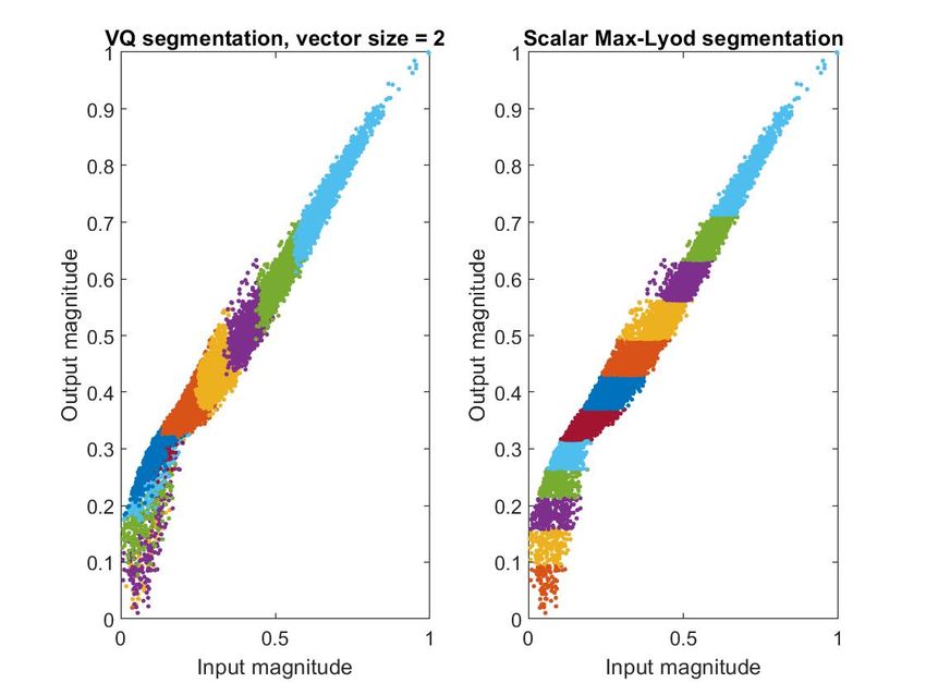
RADIOENGINEERING, VOL. 29, NO. 1, APRIL 2020                                                                                                       23

minimize the approximation error. For example, Fig. 1 shows                            The good locality of Lagrange polynomials with
the interpolation by a polynomial of degree N = 10 of the                       Tchebychev segmentation has been exploited for DPD mod-
function y = 1/(1 + x 2 ) for x ∈ [−5, +5] using a uniform                      eling by Barradas et al. in [7–9]. Details will be given
segmentation or a Tchebychev segmentation.                                      later.
      The Lagrange polynomials L N ,i (x) using Tchebychev                             Another interesting point to remind is the influence of
segmentation are interesting because their supports are well                    noisy data yi on the approximation results. It is important for
localized around points xi . So they are quasi-orthogonal                       example to better understand the influence of the measure-
which is not at all true for uniform segmentation. Figure 2                     ment noise on the PA output when training the DPD using
shows the Lagrange polynomials of degree 10 with a uniform                      indirect learning approach (see Sec. 3). It is well known
or a Tchebychev segmentation.                                                   that the noise will introduce a bias on the coefficients of the
                                                                                DPD. Suppose that the data yi are corrupted by some noise
      In the case of the approximation of a data sequence of
                                                                                i , with |i | < . The corrupted data are noted ŷi = yi + i
M samples (xk , yk ), k = 0, · · · , M − 1 with xk ∈ [a, b] by
                                                                                and the interpolation polynomial p̂. The error p̂(x) − p(x)
a polynomial p(xk ) of degree n, p(xk ) can be expressed us-
                                                                                can be bounded with Lebesgue constant that depends on the
ing different basis corresponding to different segmentations
                                                                                segmentation nodes:
of [a, b]. If we call respectively Li,Tch (xk ) and Li,Uni (xk ),
i = 0, · · · , n, the Lagrange basis with Tchebychev or uniform
                                                                                                                  n
segmentation, the approximation polynomial p(xk ) is:                                                             Õ
                                                                                            | p̂(x) − p(x)| ≤           max |Li,n (x)|.
                       n                   n                                                                            x ∈[a,b]
                                                                                                                  i=0
                      Õ                    Õ
           p(xk ) =      ci Li,Tch (xk ) =   di Li,Uni (xk ). (1)
                   i=0                     i=0                                       The Lebesgue constant max |Li,n (x)| increases with
                                                                                                                  x ∈[a,b]
Í M If a least-square           criterion is used, minimizing
                       2 , the vectors c and d containing coeffi-               the polynomial degree and is much smaller for Tchebychev
  k=1 (p(x k ) − y k ))
                                                                                segmentation than for uniform segmentation.
cients ci or di are obtained as solutions of :
                   Rc = ΦT y with R = ΦT Φ.                               (2)           Lagrange interpolation only requires that p(xi ) =
                                                                                 f (xi ) for i = 0, · · · , n. Other polynomial interpolations re-
       The matrix y is the M × 1 column vector of samples                       quest additional conditions on the derivatives of f . For ex-
yk , k = 0, · · · , M − 1, Φ is the matrix M × (n + 1) of the basis             ample, Hermite interpolation requires that the 1st derivatives
functions Φ(k, i) = Li (xk ) and ΦT is the transpose of Φ. In                   of f and p be equal at points xi . For these 2(n + 1) condi-
theory, whatever the chosen basis, the optimal solution for p                   tions, there is a unique polynomial solution p(x) of minimum
should be the same. But the condition number of the corre-                      degree 2n + 1. The approximation error e(x) = f (x) − p(x),
lation matrix R strongly depends on the basis. For example,                     for f (x) (2n + 2) times differentiable, is such that:
for a polynomial of degree n = 35, the condition number of                                 ∀x ∈ [a, b] ∃ξ ∈ (min(xi , x), max(xi , x)),
the correlation matrix R is greater than 1016 for the uniform
segmentation while it is smaller than 30 for the Tchebychev                                                                         f 2n+2 (ξ)
                                                                                           e(x) = (x − x0 )2 · · · (x − xn )2                  .
segmentation. Therefore due to those bad numerical proper-                                                                         (2n + 2)!
ties, the quality of the approximation obtained with uniform                    Hermite interpolation does not guarantee a uniform approx-
segmentation can be degraded specially when computation                         imation of f when n increases.
is done in single precision.                                                    But Bernstein polynomials associated to a continuous func-
                                                                                tion f and noted Bn f (x), converge uniformly towards f when
                                                                                the degree n increases. They correspond to a uniform seg-
                                                                                mentation and are expressed, for x ∈ [a, b] as:
                                                                                               n
                                                                                              Õ   n
                                                                                   Bn f (x) =        f (a + (b − a)k/n) (x − a)k (x − b)n−k .
                                                                                              k=0
                                                                                                  k

                                                                                The Bernstein basis polynomials of degree n are defined by
                                                                                Bk,n (x) = nk (x − a)k (x − b)n−k , k = 10, · · · , n. Figure 3
                                                                                shows Bernstein basis polynomials for n = 10 on the interval
                                                                                |−5, 5]. It can be seen that they are quite well localized around
                                                                                                                  Bk,n (x) = 1 ∀ x ∈ [a, b]. The
                                                                                                           Ín
                                                                                points xi . Also the sum k=0
                                                                                Bernstein approximation is obtained by convex linear com-
                                                                                bination which leads to good numerical properties.
                                                                                     Figure 4 shows the approximation by a polynomial of
                                                                                degree n = 10 of the function y = 1/(1 + x 2 ) for x ∈ [−5, +5]
     Fig. 1. Interpolation of y = 1/(1 + x 2 ) with an order 10 polyno-         using a Bernstein polynomial (uniform segmentation) or
             mial with uniform or Tchebychev segmentation.
                                                                                a Lagrange polynomial with Tchebychev segmentation.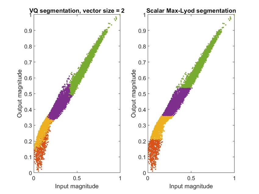
24                                  G. BAUDOIN, ON SEGMENTED PREDISTORTION FOR LINEARIZATION OF RF POWER AMPLIFIERS

                     Fig. 2. Lagrange polynomials of degree 10 with uniform (left figure) or Tchebychev (right figure) segmentation.

                                                                              2.2 Piecewise Polynomial Approximation
                                                                                   Approximation of functions by a single polynomial has
                                                                              some limitations, such as Runge’sphenomenon for Lagrange
                                                                              uniform interpolation, necessity of high polynomial degree
                                                                              polynomials leading to high computation complexity and
                                                                              potential numerical problems. Piecewise approximation is
                                                                              a way to overcome some of these limitations. It allows to
                                                                              take advantage of the regularity of the function in a limited
                                                                              region.
                                                                                      To approximate a function y = f (x), x ∈ [a, b], the ba-
                                                                              sic idea of piecewise polynomial approximation is to partition
     Fig. 3. Bernstein polynomials of degree 10.                              the interval [a, b] in N segments over which f is approximated
                                                                              by a polynomial. As the segments are shorter than the length
                                                                              of [a, b], f should have a more regular shape on each local
                                                                              segment than on the global interval and it should be possi-
                                                                              ble to use polynomials of smaller degree than for the global
                                                                              polynomial approximation. Without additional constraints,
                                                                              the piecewise approximation may be discontinuous. Gener-
                                                                              ally, some regularity is required for the approximation and
                                                                              a popular approach is the approximation by spline functions.
                                                                              There are two different ways to present splines. The first one
                                                                              consists in considering piecewise polynomials with continu-
                                                                              ity constraints on the function and its first derivatives at the
                                                                              borders of the segments. In this first approach the regularity
                                                                              constraints can be different for the different nodes. The sec-
                                                                              ond approach is based on a trade-off between the accuracy of
     Fig. 4. Approximation of y = 1/(1+ x 2 ) with order 10 Bernstein         the approximation and its regularity. In the second approach,
             or Lagrange (Tchebychev segmentation) polynomial.                the natural splines solution is obtained for a set of N data
                                                                              (xi , yi )i=1
                                                                                        N by approximating f by a function h optimizing the

                                                                              criterion:
      On this example, it can be seen that the approximation
                                                                                                 N                    ∫ b
error obtained with the Bernstein polynomial is larger than                                   1 Õ
that obtained with Lagrange interpolation and a Tchebychev                                min       (yi − h(xi )) + λ
                                                                                                                 2
                                                                                                                          (h m (x))2 dx
                                                                                            h N                        a
                                                                                                i=1
segmentation. But there is no Runge’s phenomenon in the
Bernstein approximation and, if f (x) is continuous, it con-                  where λ > 0 is a smoothing constant. The solution of this
verges uniformly (even if rather slowly) towards f (x) which                  problem is a piecewise function made of polynomials of de-
is not true for Lagrange interpolation. An interesting way                    gree 2m − 1 in segments defined by boundaries xi and sat-
to obtain a faster convergence of the approximation is to use                 isfying continuity at the boundaries for the function and its
piecewise approximation.                                                      2m − 2 first derivatives. With m = 2, this gives cubic splines.
RADIOENGINEERING, VOL. 29, NO. 1, APRIL 2020 25
A function h(x) is a polynomial spline of order d + 1 in
[a, b] if h ∈ C (d−1) (C (d−1) space of functions with d − 1 con-
tinuous derivatives) and for a given set s of non-decreasing
segmentation values (knots) (a = x0, x1, · · · , xn−1, xn = b),
h(x) is a polynomial pi (x) of degree d on each segment
[xi , xi+1 [. We note Sd,s the set of all spline functions of
order d + 1 for the set of knots s. A cubic spline corre-
sponds to the case d = 3. For a cubic spline, pi (x) =
ai x 3 + bi x 2 + ci x + di , x ∈ [xi , xi+1 [ and pi (x) ∈ C 2 [x0, xn ],
0 0
with the conditions pi−1 (xi ) = pi (xi ), pi−1 (xi ) = pi (xi ),
p”i−1 (xi ) = p”i (xi ), i = 1, 2, · · · , n − 1. Cardinal splines corre-
spond to an infinite number of knots with unit spacing.
With cubic interpolation, for a given set (xi , yi )i=0
n , there
are 4n coefficients (ai , bi , ci , di )i=0 to determine and a set of
n−1
n + 1 linear equations h(xi ) = yi plus 3(n − 1) continuity Fig. 5. Cubic B-splines (top with 9 knots) or spline basis of [11]
equations which gives a total of 4n − 2 linear equations. So (bottom) with uniform segmentation.
there are 2 possible degrees of freedom that correspond to
different types of splines. For example, natural splines are Splines functions can be used to approximate functions
defined by setting h” (x0 ) = 0 and h” (xn ) = 0. Natural splines generally defined by a set of data points. The approximation
minimizes the integral of the squared second derivative of h. can be based on interpolation or on minimizing a given crite-
Sd,s is a vector-space of dimension n+ d. An interesting rion. A commonly used approximation criterion in the field
basis is that of B-splines (Basis-spline) [10]. B-splines are of DPD is the least-square criterion. The approximation by
splines functions with minimum support [xi , xi+d+1 [. They a spline function with LS criterion can be achieved as in (1)
can be defined by a recurrence relation for a given degree and (2). in the case of the approximation of a data sequence
of polynomials d and a partition s of the interval [a, b] with of M samples (xk , yk ), k = 0, · · · , M − 1 with xk ∈ [a, b]
n + 1 knots and n > d + 2. The recurrence relation defining by a spline function h(x) of degree d and segmentation s,
the i th B-spline of degree d, noted Bi,d,s (∀x ∈ R) is: h(x) can expressed as a linear combination of B-splines with
coefficients ci :
x − xi xi+1+d − x
Bi,d,s (x) = Bi,d−1,s (x) + Bi+1,d−1,s (x).
xi+d − xi xi+1+d − xi+1
Õ
h(x) = ci Bi,d,s (x).
1, if xi ≤ x < xi+1
Bi,0,s (x) = Xi (x) = i
0, otherwise.
ÍM
(h(xk ) − yk )2 , the vector c of coef-
Õ
And Bi,0,s (x) = 1 ∀ x. For LS critera min k=1
i ficients ci is obtained as the solution of (3), where y is the
The B-spline Bi,d,s can be expressed as a concatenation M × 1 column vector of samples yk , k = 0, · · · , M − 1 and
of d + 1 successive polynomials pieces of degree d. It is Φ is the matrix M × (n + 1) of the B-spline functions.
equal to 0 outside the segment [xi , xi+d+1 [. And Bi,d,s = 0
if xi = xi+d+1 . On any interval [xi , xi+d+1 [, at most d + 1 Rc = ΦT y with R = ΦT Φ. (3)
B-splines are different from 0: (Bi−d,d , · · · , Bi,d ). For a finite
set of knots in a finite interval [a, b], there are n − d B-splines
whose support is completely included in [a, b]. To obtain
a full basis of B-splines functions on [a, b], we must had 3. Generalities on DPD
2d basis-functions whose support is partly inside [a, b], with
A general presentation of digital predistortion can be
usually d nodes equal to a and d nodes equal to b. A knot
found in [1]. Figure 6 shows a basic tansmitter architecture
has a multiplicity m if it is repeated m times in the sequence.
using adaptive DPD.
Any spline function hd,s can be written as a linear com-
bination of B-splines: I (n )
Digital Analog
Predistorter
y(t )
Õ DAC RF PA
upconverter
hd,s (s) = ci Bi,d,s (x). Q( n )
(FPGA)
i
DSP
Figure 5 shows an example of cubic B-splines defined
for x ∈ [0, 1] with a uniform segmentation and a sequence Dual/Single ZIF/IF
ADC downconverter
of 9 knots. The basis functions are well localized around
the knots and are therefore quasi-orthogonal. It also shows
another spline basis proposed in [11] that keeps a very short
Fig. 6. Transmitter architecture with DPD.
support when d increases.26 G. BAUDOIN, ON SEGMENTED PREDISTORTION FOR LINEARIZATION OF RF POWER AMPLIFIERS
Volterra based models are very common for DPD. Most DLA approach tries to minimize a criterion based on
of them can be expressed as a linear combination of regres- the error eDLA (n) = x(n) − y0 (n) where x is the DPD input
sors that are derived from the input signal z(n). For example, and y0 (n) = y(n)/G is the normalized output with a reference
for the generalized memory polynomial model (GMP) , the gain G (Fig. 7). Many of DLA algorithms are based on first
output y(n) is expressed as: identifying the PA model and then inverting it or use it to
train the DPD.
a −1 LÕ
KÕ a −1
ILA approach (Fig. 8) is based on first solving a post-
y(n) = ak,l z(n − l)|z(n − l)| k distortion problem and then using the postdistorter as a pre-
k=0 l=0
distorter. The postdistorter is a fictive block placed after
b −1 Õ
K b LÕ Mb
Õ the PA that corrects the normalized PA output in order to
+ bk,l,m z(n − l)|z(n − l − m)| k
minimize a criterion based on error eILA = (z(n) − w(n))
k=1 l=0 m=1
where z in the PA input and w(n) Í is the postdistorter output
c −1 Õ
K c LÕ Mc
Õ (Fig. 8). Using a LS criterion J = i=n−N n 2
+1 |eILA (n)| on N
+ ck,l,m z(n − l)|z(n − l + m)| k . (4)
observation samples correponding to the PA output and input
k=1 l=0 m=1 n
(y0 (i), z(i))i=n−N +1 , the coefficients of the postdistorter that
minimize J are solutions of a linear set of equations. The op-
It can be written as a dot product between the Nc ×1 vec- timum coefficients vector is obtained with the pseudo-inverse
tor d of all the coefficients (ak,l , bk,l,m, ck,l,m ) and the Nc × 1 of the regression matrix Φy0 built on y0 (5).
regressor vector φ z (n), with y(n) = φ Tz (n)d. The regressor
vector φ z (n), built on z, contains the different basis functions
(z(n−l)|z(n−l)| k , z(n−l)|z(n−l −m)| k , z(n−l)|z(n−l +m)| k ).
ΦHy0 Φy0 d = Φy0 z,
H
For a set of N signal samples, the column vector y =
(y(n), · · · , y(n − N + 1))T is equal to:
−1
d = ΦH y0 Φ y0 ΦH
y0 z (5)
y = Φz d, with
T where ΦH
y0 is the hermitian transpose of Φy0 .
Φz = φ z (n), φ z (n − 1), · · · , φ z (n − N + 1) ,
ILA approach is popular because the coefficient iden-
φ z (n) = (φ1 (n), φ2 (n), · · · , φ Nc (n))T . tification is a linear optimization problem. However, the
measurement noise at the output of the PA introduces a bias
where Φz is the N × Nc matrix of regressors, φi (n) is the i th on the solution. The DLA approach does not suffer from this
basis function, Nc is the number of coefficients. drawback but it leads to a nonlinear optimization problem.
There are two general approaches for the identification Both approaches depends on matrix R = ΦH y0 Φy0 . Un-
of coefficients, namely the direct (DLA) and the indirect fortunately, the successive signal samples are usually cor-
learning (ILA) approaches. related and therefore matrix R is badly conditioned, espe-
cially when the the nonlinearity orders are high. To manage
this problem, different methods can be used: regulariza-
tion techniques such as L2 norm Tikhonov (ridge regres-
sion), orthogonal polynomial basis, orthogonalization (e.g.
Gram-Schmidt technique), dimension reduction by suppress-
ing less-significant basis functions (e.g. orthogonal matching
pursuit algorithm (OMP)). Another possible approach is to
segment the problem into several problems of smaller di-
Fig. 7. Principle of DLA direct learning approach. mensions. Different types of segmented DPD have been
proposed. They are presented in the following sections.
4. Segmented DPD with Functions of
a Single Real-Valued Variable
We have seen in Sec. 2 some results about interpolation
or approximation of functions by polynomials or piecewise
polynomials in the case of functions of a single real-valued
variable. But in general, DPD are not such simple func-
tions. First the input signal is complex-valued and secondly
the DPD has to take into account the memory effects of the
Fig. 8. Principle of ILA direct learning approach. PA. It is ruled by nonlinear differential equations. It can beRADIOENGINEERING, VOL. 29, NO. 1, APRIL 2020 27
simplified by considering that the memory length is finite. quantized value of some companding function of the input.
The DPD can then be represented by a multivariate function N −1 the different possible quantized values,
If we note (xk )k=0
of complex-valued variables. The complexity is much higher the LUT contains the corresponding gain GPD,k = GPD (xk ).
than for a function of a single real-value input variable. For an input value x, the corrective gain is obtained by some
interpolation or approximation of the function GPD (x) from
Fortunately there are several cases, where simplifica-
the data (xk , GPD (xk )).
tions can be done allowing to represent the nonlinear aspects
of the DPD by a simple single-variable function of a real In order to cope with complicated PA characteristics,
variable. This is object of the next two sections. it is possible to increase the polynomial order or the LUT
size but at the price of introducing ripples in the function
(Runge phenomenon), increasing training convergence time,
4.1 Piecewise Modeling in Quasi-Memoryless
Models complexity and numerical problems. Therefore, different
segmented approaches have been proposed: piecewise linear
In this section we will address the cases of quasi- regression of the AM/AM and AM/PM of the PA gain [14],
memoryless models and of block oriented models separating piecewise polynomial modeling of AM/AM and AM/PM in
nonlinearity from memory effects. These are special cases two regions (with a high order polynomial for the saturation
where single-variable real-valued functions can be used for region and a low order one for the linear region) [15], cubic
the DPD model. spline interpolation [16], [17], piecewise interpolation by arc
The first works on DPD were dedicated to signals with of circles [18], piecewise bilinear rational function [19] of
narrow bandwidths for which PA memory effects could be the PA gain with piecewise inverse of the PA model to obtain
neglected. In that case, the quasi-memoryless PA can be the DPD model. An advantage of piecewise linear and piece-
modeled with its AM/AM and AM/PM characteristics as wise bilinear function is that they can be easily inverted. For
functions of the magnitude (or power) of the input signal example, in the case of a bilinear function, if the PA model,
z(n). The baseband equivalent of the PA output can be ex- for an input z and an output y is defined by:
pressed as y(n) = GPA (|z(n)|)z(n) where the magnitude and
the phase of the gain GPA respectively represent the AM/AM ai |z| + bi φi |z| + ψi
|y| = , arg(y) = arg(z) +
and AM/PM of the PA. A major breakthrough was realized ci |z| + di θ i |z| + ηi
by Cavers [12] who proposed to model the DPD as a simple |z| ∈ Ri , i ∈ {1, 2, . . . , N } where Ri is the segment N o i.
complex gain GPD depending only on the magnitude of the
input signals and allowing to compensate for the AM/AM the inverse model used for the DPD (with input x and output
and AM/PM distortion of the PA. So, the output z(n) of the z) is given by:
DPD, for an input signal x(n) can be written as:
z(n) = GPD (|x(n)|)x(n), with x(n) = |x(n)| exp(jφ x (n)), di |x| − bi φi |z| + ψi
|z| = , arg(z) = arg(x) − .
GPD (|x(n)|) = |GPD (|x(n)|)|ejθPD ( |x(n) |), −ci |x| + ai θ i |z| + ηi
z(n) = |x(n)| |GPD (|x(n)|)| ej(φ x (n)+θPD ( |x(n) |)) .
In most of those studies, the segmentation (number of
The DPD complex gain should pre-compensate the PA gain segments, position of the knots) and degrees of polynomial
so that the PA output be proportional to the input signal x segments are determined in an empirical way. In [20], authors
with a reference gain G, which means: use AM/AM derivatives to segment it into linear, nonlinear
and saturation regions.
y(n) = GPA (|z(n)|) z(n) = GPA (|z(n)|) GPD (|x(n)|) x(n)
= G x(n) ∀x(n). Cavers worked on the optimal LUT-spacing [21]. He
derived the optimum companding function of input magni-
So: GPA (|x(n) GPD (|x(n)|)|) GPD (|x(n)|) = G, ∀x(n). tude for table indexing. It depends on the signal statistics and
The DPD corrective complex gain can be implemented on PA characteristics. He showed that for a class AB PA,
by a Look-up-Table (LUT) [12] or by a polynomial func- equispacing by amplitude is closed to the optimum. In [22],
tion [13]: authors propose a non-uniform LUT indexing function that
K
allows for a signal to quantization noise that does not de-
pend on input signal statistics or power backoff of the PA.
Õ
GDPD (|x(n)|) = ak |x(n)| k−1 . (6)
k=1
In [23] a segmented approach is used with more LUT en-
tries in the strongly nonlinear segments than in the linear
The content of the LUT or the coefficients of the poly-
ones. In [24] the LUT-spacing is dynamically optimized in
nomial are adaptively updated by DLA or ILA. In practice,
function of online estimated PA characteristics and the input
either the DPD is directly updated or the PA gain is first
signal statistics using histograms to approximate the signal
estimated and then inverted to obtain the DPD.
statistics. In [25] and in [26], the authors theoretically study
For polynomial DPD, the DPD output is directly ob- respectively the optimal spacing of piecewise linear LUT
tained by (6). For the LUT case, the LUT is addressed by the DPD and of a quadratically interpolated LUT DPD.28 G. BAUDOIN, ON SEGMENTED PREDISTORTION FOR LINEARIZATION OF RF POWER AMPLIFIERS
4.2 Piecewise Modeling in Block-Oriented In [33], we proposed a BONL DPD called "Filtered
Models LUT" or FLUT. The FLUT DPD is made of an SNL block
followed by a linear filter. But at the difference of Hammer-
In order to take into account PA memory effects, one stein models, the filter coefficients vary with the magnitude
possible approach is to use block oriented nonlinear mod- of the DPD input signal. The SNL block is implemented by
els (BONL) separating nonlinearity from memory effects a linear piecewise LUT (gain-LUT). A codebook stores the
such as Wiener, Hammerstein, Wiener-Hammerstein mod- coefficients of the different filters. Both the gain-LUT and
els. These models associate in cascade or in parallel several the codebook of filters are indexed by the magnitude of the
linear time-invariant filters (LTI) that represent the dynamics input signal with a uniform companding function.
of the system and static nonlinear (SNL) blocks. A Wiener
model is made of a cascade of an LTI followed by an SNL
block and an Hammerstein model of an SNL block followed
4.3 Piecewise Modeling in Volterra Based
by a linear filter. One drawback of BONL models is that
Models
the identification of their parameters has to be done by non- Models derived from Volterra or from dynamic Volterra
linear optimisation technique. But an interesting point is series can be reformulated (or generalized) with nonlinear
that SNL blocks can be represented as complex gains that single-variable functions of the input-signal magnitude.
are single-variable functions of their input signal magnitude. For example, an MP DPD model with input x and output
And therefore, all the piecewise techniques presented in 4.1 z defined as:
can be applied to the SNL blocks of BONL models.
K−1
ÕÕ L−1
In [27], the PA is modeled by a Wiener model where z(n) = ak,l x(n − l)|x(n − l)| k ,
the SNL block is represented by a simplicial canonical piece- k=0 l=0
wise linear (SCPWL) function [28]. Two SCPWL functions can be reformulated with L single-variable nonlinear func-
are used respectively for AM/AM and AM/PM characteris- tion fNL,l as:
tics. The DPD is an Hammerstein model. The inverse of
the SNL-block of the PA model is also a piecewise linear L−1 K−1
!
Õ Õ
function that can be easily obtained by inverse coordinate z(n) = x(n − l) ak,l |x(n − l)| k
mapping. In [29], a piecewise linear predistorter is also pro- l=0 k=0
posed. the parameters of the SNL block are estimated by L−1
Õ
particle swarm optimization (PSO). = ak,l x(n − l) fNL,l (|x(n − l)|).
l=0
In [30], the authors apply a Wiener model to the PA. The
These single-variable nonlinear functions fNL,l can be ap-
SNL block of the PA Wiener model comprises an AM/AM
proximated by different piecewise functions; A DPD model
characteristic that is modeled by a piecewise linear continu-
where the fNL,l are modeled by complex-valued cubic splines
ous and monotonically increasing function and an AM/PM
is proposed by Safari et al. in [34] and compared with MP
characteristic represented by a piecewise constant function.
model. The obtained piecewise model is linear with respect
The segmentation is determined empirically. The DPD is
to its coefficients and can be identified using LS criterion and
modeled by a memory polynomial model. A direct learning
by ILA approach with similar equations as (3) and (5). It
adaptive DPD is proposed. First the PA model is identi-
shows better results than MP model for a smaller number of
fied using RLS (recursive least square) algorithm. There
coefficients. The same kind of approach is proposed in [35]
are two parameters to identify for each segment of the SNL
using 2nd order nonlinearity piecewise MP and a single knot.
block. The inverse of the PA model is easy to obtain. It is
an Hammerstein model with a piecewise SNL block. The The same method can be applied to reformulate GMP,
DPD parameters are obtained by a piecewise RLS (PRLS) DDR or any other Volterra based models. The principle is to
algorithm. The error to minimize is calculated thanks to the first do the summation on the nonlinearity orders. In a GMP
inverse function of the PA. This segmented approach leads model, each of the 3 terms of (4) can be reformulated in the
to a direct learning adaptive algorithm that is less complex same way, e.g., for the second term:
than common direct learning algorithms but it offers the same
b −1 Õ
K b LÕ Mb
level of performance. Õ
bk,l,m u(n − l)|u(n − l − m)| k
k=1 l=0 m=1
In [31], two Hammerstein models with Catmull-Rom
b −1 Õ
LÕ Mb Kb
!
cubic spline static nonlinearity are used for the DPD. One Õ
for correcting AM/AM distortion and the other for correct- = x(n − l) bk,l,m |u(n − l − m)| k
l=0 m=1 k=1
ing AM/PM distortion. The DPD coefficients are identified
b −1 Õ
LÕ Mb
using ILA with a separable nonlinear least squares (SNLS)
= x(n − l) fNL,l,m (|x(n − l − m)|).
optimization [32]. The segmentation is optimized empiri-
l=0 m=1
cally. The approach allows to compensate for high-degree
nonlinearity with a limited set of coefficients. There are M L single-variable nonlinear functions fNL,l,m .RADIOENGINEERING, VOL. 29, NO. 1, APRIL 2020 29
Barradas et al. in [9] show how this approach can be functions for nonlinearities. These approaches partition the
applied to any Volterra based model. They approximate the global space of the input signals and fits a piecewise DPD
fNL,l,m by cubic splines functions constructed with B-splines. to each of the regions of the partition. In this section, we
They suggest to use Tchebychev nodes as splines knots. They present three techniques: Vector-Switched (VS) DPD, Con-
show that the numerical stability (matrix conditionning) of tinuous Piecewise Linear (CPWL) DPD and Decomposed
ILA identification with this approach is much better than Vector Rotation (DVR).
with GMP model for similar performance and complexity.
In [7] they expound that the high locality (limited support) of 5.1 Switched DPD
nonlinear splines basis makes them quasi-orthogonal which
explains their better numerical properties. They develop their Switched DPD allows to derive piecewise DPD taking
analysis by a theoretical comparison of polynomial and LUTs into account nonlinearity and memory effects and applying
in PA modeling. the segmentation in both domains. The principle consists
in switching several DPD models, each of them being well
This approach is applied in [36] with fNL,l,m functions
suited to a specific segment (or region) of the input signal.
approximated by piecewise Lagrange (APL) basis functions.
The continuity between the different models is a delicate
Authors of [37] consider the determination of DPD as notion. There are at least two questions: how should this
a multivariate regression problem and use the fact that any continuity be defined and is it really necessary. Indeed, we
multivariate function can be approximated by a sum of sep- can consider continuity with time and continuity with mag-
arable functions to express a very general form of DPD with nitude. When the models include some kind of memory,
single-variable real-valued nonlinear functions. These func- the final condition of one model can be used as the initial
tions can then be piecewise approximated by splines. conditions of the next model, which ensures some kind of
temporal continuity.
In [38], Zhu et al. propose a different approach to cope
with envelop tracking PA, the behavior of which changes Switched DPD allows to use in each region a DPD
significantly in functions of power region. The technique model of smaller complexity (nonlinearity orders, memory
is called "Decomposed Piecewise Volterra Series". It is lengths) than would be necessary with a global model. It has
based on vector threshold decomposition of the input sig- the ability to represent hard nonlinearities and to identify the
nal x(n) = |x(n)|ejφ . It was initially proposed by Heredia for region-DPD models with good numerical stability.
real-valued signals in [39]. For a given set of real positive
N and λ = 0, N sub-signals x In [42], Afsardoost et al. propose the vector-switched
increasing thresholds (λi )i=1 0 i
(VS) DPD model. the VS model is a set of DPD mod-
are obtained, with:
els that can be switched and applied to the input according
0,
|x(n)| ≤ λi−1 to some switching function based on the region of the in-
xi (n) = (|x(n)| − λi−1 )ejφ , λi−1 < |x(n)| ≤ λi
put signal. The space of input signals x(n) is partitioned
(λi − λi−1 )ejφ ,
|x(n)| > λi into N regions using vector quantization (VQ). VQ is ap-
N plied to vectors of Q successive complex input samples
X(Q) (n) = {x(n), x(n − 1), . . . , x(n − Q + 1)}. For an in-
Õ
with x(n) = xi (n).
i=1 put sample x(n), the class of X(Q) (n) is determined and the
Every sub-signal is processed by a specific sub-DPD model corresponding model is chosen for x(n). Authors note that it
(here DDR models are used). And the outputs of all is generally sufficient to use Q = 2 and to apply VQ on the
these DPD are summed to obtain the global predistorted input magnitude only.
signal. In [40], the authors apply GMP models for the Authors of [41] apply this approach with a set of GMP
sub-DPD and the thresholds are determined using the models and a learning algorithm that decorrelates the GMP
slope and the rate of slope of the AM/AM characteris- polynomial basis functions. This training is applied on each
tic. In [41], the same technique is used with a learning DPD model independently using the input samples of the
algorithm that decorrelates the DDR polynomial basis func- corresponding region. The VQ segmentation is achieved on
tions and is applied on each sub-DPD independently. the magnitude of the input signal with Q = 1 .
5. Segmented DPD for Nonlinearity 5.2 From PWL to Memory-SCPWL DPD
and Memory Domains Piecewise linear functions and in particular simplicial
canonical piecewise linear (SCPWL) functions were first ap-
In Sec. 4, the segmentation is applied on the nonlin- plied to approximate functions of a single real-variable vari-
earities only. But for some types of PA, e.g. Doherty PA, able such as those presented in Sec. 4, in static cases to model
the memory effects are different at different power levels. In AM/AM and AM/PM characteristics of quasi-memoryless
such cases, it may be useful to also segment the memory do- PA [43], [44] or in dynamic cases to represent nonlinearities
main. In this section, we present different approaches that are functions in Volterra based models [45]. Then they were
not limited to the piecewise approximation of single-variable also used to model functions of complex input [46] with the30 G. BAUDOIN, ON SEGMENTED PREDISTORTION FOR LINEARIZATION OF RF POWER AMPLIFIERS
name memory-SCPWL functions. A PWL representation where L is the memory length. The hyperlanes are defined
ak,l x(n − l) − βk = 0.
ÍL
has several interests. In particular, thanks to its linear affine by l=0
property, it can be inverted very easily. A PWL function can
CPWL can approximate a wide range of continuous
be described segment per segment, which may require a large
nonlinear function with a very good accuracy [50]. Unfortu-
number of coefficients. The number of coefficients can be
nately, this model is not linear with respect to its coefficients
reduced by using a global representation called Canonical
(al , b, ck ) and it is not directly usable for complex-valued input
PWL (CPWL) function [47] or an even more compact form
signal x. To overcome these two limitations, Zhu proposed
called Simplicial Canonical PWL (SCPWL) function [28].
a new formulation:
A SCPWL function f of a single real-variable x, is given by:
L
σ−1 Õ
y(n) = al x(n − l) + b
Õ
f (x) = c0 + ci λi (x), x ∈ R
i=1 l=0
K Õ
L
where σ is the number of segment breakpoints, ci are coef-
Õ
+ ck,l ||x(n − l)| − βk | ej arg (x(n−l)) .
ficients, and λi (x) are basis functions defined with a set of k=1 l=0
increasing breakpoints values (βi )i=1σ by:
In order to introduce interaction between signals at different
(x − βi + |x − βi |), x < βσ
1
time instants, some other terms can be added to the model.
λi (x) = 12
2 (βσ − βi + | βσ − β i |), x ≥ βσ . Depending on these added terms, the model is more or less
complex. One possible expression is:
The coefficients ci can be complex-valued.
L
Cheong et al. in [46] modified that expression to make Õ
y(n) = al x(n − l) + b (8)
it suitable for modeling nonlinearities and memory effects.
l=0
For a given memory length L, considering the last L input K Õ
L
samples (x(n − l))l=0 L , the new form is: Õ
+ ck,l,1 ||x(n − l)| − βk | ej arg (x(n−l))
σ−1
L
" #
Õ Õ k=1 l=0
f (x) = cl,0 + cl,i λi (|x(n − l)|)ej arg(x(n−l))
. (7) K Õ
Õ L
l=0 i=1 + ck,l,21 ||x(n − l)| − βk | ej arg (x(n−l)) |x(n)|
This new form is linear with respect to its coeffi- k=1 l=0
K Õ
L
cients cl,i which simplifies its identification. Replacing Õ
|x − βk | where x is real-valued by ||x| − βk |ej arg (x) where + ck,l,22 ||x(n − l)| − βk | x(n)
x = |x|ej arg (x) is complex-valued, is called Decomposed Vec- k=1 l=1
K Õ L
tor Rotation (DVR). Authors of [46] compared the memory- Õ
+ ck,l,23 ||x(n − l)| − βk | x(n − l)
SCPWL DPD with MP and GPM DPD. They showed that
k=1 l=1
memory-SCPWL DPD offers better modeling accuracy for
K Õ L
sharp nonlinearities and that it is less sensible to noise at PA Õ
+ ck,l,24 ||x(n)| − βk | x(n − l) + . . .
output thus reducing the potential bias on coefficients for ILA
k=1 l=1
identification.
Experimental tests on envelop tracking and doherty PA have
Of course, CPWL functions can also be used with the
shown the very good performance of DVR models. In those
generalized form of Volterra DPD using function of single
tests the threshold βk were fixed and uniformely spaced. But
real-valued variables [48].
an optimization of their values should improve the results.
In [51], Zhu discusses the respective interests of
5.3 Decomposed Vector Rotation (DVR) Mod-
Volterra series and CPWL functions for DPD.
els for DPD
Zhu [49] has extended the memory-SCPWL model Authors of [52] propose a modification of the DVR
given by (7) with a more general model called Decomposed model avoiding the calculation of absolute values. And the
Vector Rotation DVR model. It starts from the represen- same kind of modified model is used in [53] for linearization
tation by CPWL of a finite memory nonlinear system with of radio over fiber link.
real-valued input and output signals z and y. CPWL achieves
a partition of the input signal space into K polyhedral regions
separated by hyperplanes whose boundaries are defined with 6. Advanced Segmented DPD for
K . The input-output relation is expressed
thresholds (βk )k=1
as:
Multidimensional DPD
L K L
In this section, we briefly discuss some more advanced
points such as application of segmented DPD to systems us-
Õ Õ Õ
y(n) = al x(n − l) + b + ck ak,l x(n − l) − βk
l=0 k=1 l=0
ing carrier aggregation with concurrent multi-band transmit-RADIOENGINEERING, VOL. 29, NO. 1, APRIL 2020 31
ters or MIMO techniques. Both cases correspond to multiple- (|x1,u | 2, |x2,v | 2 ), the basis functions φ j,k (|x1 | 2, |x2 | 2 ) are cre-
inputs DPD (or multidimensional DPD). ated with 2D interpolation cubic spline such that:
In systems using carrier aggregation with concurrent
φ j,k (|x1,u | 2, |x2,v | 2 ) = δ j,u δk,v
multi-band transmitters, the input signal includes several fre-
1 ∀( j, k) = (u, v)
quency bands that can be widely spaced in the non-contiguous =
intra-band or inter-band aggregation. It is possible to con- 0 ∀ other knots.
sider the multi-band signal as a unique one-dimensional (1D)
single-band signal and to design the DPD accordingly but it The 2D cubic spline basis are built from 1D Cubic spline
will result in the use of very high sampling frequency and lead basis by tensor product. The number of coefficients is equal
to very high complexity. Another better approach consists in to M Ns1 Ns2 .
splitting the 1D signal into N sub-signals corresponding to
each of the N band. This is a segmentation in the frequency In [57], instead of segmenting the model using single
domain. The sub-signals have a much narrower bandwidth input magnitude, the partioning is done using vector quan-
than the 1D original signal and can be separately digitized at tization on combined input magnitudes. In [58], [59], 2D
a reasonable sampling rate. Separate feedback paths are used CPWL models are proposed.
for the different sub-signals. Most often, N = 2 or 3. The The case of DPD for MIMO transmitters is quite sim-
N-dimension DPD must take into account the different sub- ilar to that of multi-band transmitters. nonlinear crosstalk
signals to construct the predistorted signals corresponding to effects due to coupling at the inputs of the elementary PAs
each carrier and suppress the cross-distortion generated be- create cross-modulation of the elementary signals. In [60],
tween the sub-signals [54]. For example, for a 2D-DPD with multivariate polynomial models are used. To reduce the
two input sub-signals x1 and x2 and two output predistorted complexity of such DPD, different piecewise approaches are
sub-signals z1 and z2 , a possible DPD model is: studied. For example in [61], [62] Dual-Input Canonical
Piecewise-Linear DPD are presented for MIMO applications
M−1 N Õ
k
ÕÕ
(1) with two antennas.
z1 (n) = ck, x (n − m)|x1 (n − m)| k−j |x2 (n − m)| j
j,m 1
m=0 k=0 j=0 A new promising approach for multidimensional DPD
M−1
ÕÕ N Õk with Multiple input multiple outputs, called Tensor-Network-
(2)
z2 (n) = ck, j,m x2 (n − m)|x2 (n − m)| |x1 (n − m)| .
k−j j Based DPD, is proposed in [63]. This new development
m=0 k=0 j=0 should facilitate the identification of Volterra series with
very high memory lengths and memory orders. They are
based on the tensor-network based MIMO Volterra system
This multi-dimensional MP model have a large num-
framework of [64].
ber of coefficients. Therefore it can be interesting to use
piecewise models to decrease the number of necessary coef-
ficients. Naraharisetti et al. [11], [55] have reformulated the
model in a more general form that is expressed for zi with 7. Experimental Comparisons
i = 1 or 2 as: In this section, we give some experimental compar-
M−1 isons of three types of DPD: a non-segmented GMP model,
a vector-switched DPD and a DVR DPD.
Õ
zi (n) = G(i)
m |x1 (n − m)| , |x2 (n − m)|
2 2
xi (n − m).
m=0 The experiments have been done with a strongly non-
linear 3-way Doherty PA based on three LDMOS transistors
The nonlinear gain functions G(i) m are functions of the two (BLF7G22LS-130 from Ampleon). Its maximum peak out-
real-valued signals |x1 | and |x2 |. They can be approximated put power is 57 dBm. Its linear gain is 16 dB. The PA is
by different piecewise functions and in particular using spline preceded by a driver with a gain of 31.5 dB. The used car-
basis functions. rier frequency is 2.14 GHz. The input signal is an LTE with
2D cubic splines basis are used in [11], [55] and ex- a bandwidth of 20 MHz and a PAPR of 8 dB. The tests were
tended to 3D cubic spline basis in [56]. The coefficients of achieved at an average PA output power equal to 47.3 dBm.
the cubic spline basis are obtained by LS fitting of the mea- For the presented results, training has been done with ILA.
sured data. Using the cubic spline basis functions φ j,k , the
gain functions are approximated by: 7.1 Non-Segmented GMP-DPD
Õ Ns2
Ns1 Õ The structure of the GMP model (values of the eight
G(i) |x1 | 2
, |x2 | 2
= ci(m) φ (|x1 | 2, |x2 | 2 ). parameters (Ka, La, Kb , Lb , Mb , Kc , Lc , Mc )) is determined
m jk j,k
j=0 k=0 by an hill-climbing (HC) optimization algorithm that we
proposed in [65]. This algorithm optimizes a trade-off
Naraharisetti proposed the following formulation for the between the number of coefficients and the accuracy of
splines basis [11], [55]. For a given set of 2D-knots the model. The obtained GMP structure is given by:32 G. BAUDOIN, ON SEGMENTED PREDISTORTION FOR LINEARIZATION OF RF POWER AMPLIFIERS
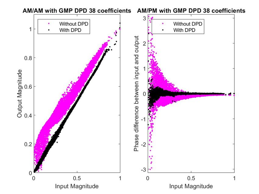
(Ka = 11, La = 2, Kb = 4, Lb = 1, Mb = 1, Kc = 3, Lc =
4, Mc = 1). It has 38 coefficients. The obtained normalized
mean square error (NMSE) is equal to −32.7 dB. NMSE is
defined as the ratio between the power of the error and the
power of the output signal. The AM/AM and AM/PM charac-
teristics with and without the GMP DPD are given in Fig. 9.
To improve the results, we can try to increase the num-
ber of coefficients to the detriment of complexity. But the
HC algorithm shows that the results cannot be significantly
improved by increasing the number of coefficients. For exam-
ple with 80 coefficients, the NMSE is only equal to −33.9 dB
(only 1 dB better than with 38 coefficients).
By inspection of the AM/AM characteristic, we can
clearly distinguish different areas with different slopes
(gains). The segmented approaches may be good candidates Fig. 9. AM/AM and AM/PM characteristics with and without
to improve performance without significantly increasing the the GMP DPD (38 coefficients).
complexity.
7.2 Vector-Switched DPD (VS-DPD)
To apply Switched-Vector DPD with have to determine
the good segmentation and the structures of models in each
segment. We have chosen GMP models for each segment
(or VQ class) with 14 coefficients and a maximum order of
nonlinearity equal to 5 (instead of 38 coefficients and a maxi-
mum nonlinearity of 11 in the global GMP model). We used
the same structure for all of the segment-models because the
FPGA implementation will be sized by the most complex of
those structures.
We have compared several types of segmentation:
Fig. 10. Influence of the number of segments on NMSE.
• scalar uniform quantization, scalar non-uniform Lloyd-
Max segmentation,vector-quantization (VQ) with dif- Figure 10 illustrates how varies the NMSE in function
ferent vector dimensions, of the number of segments NS for different types of quan-
tization and VQ vector dimension. It can be seen that for
• training of the segmentation codebook on the PA input scalar quantization and NS > 10 , using Lyod-Max quantizer
or output signal, instead of uniform segmentation only slightly improves the
results. But using VQ segmentation with a vector size equal
• segmentation determined by the signals or by the PA to 2 or 3 instead of scalar segmentation, improves the NMSE
characteristics. by approximately 1 dB. A vector size equal to 2 is sufficient.
The results improve slowly when increasing the number of
For each type of segmentation, with have tested different classes but this number must remain small enough in order
values for the number of segments that in each training buffer of N samples, the population size
of each class is large enough for a good identification of the
We observed that segmentation determined by the sig-
class-model. On the same Fig. 10, we have added the result
nals gives better results than segmentation driven by PA char-
obtained by the global GMP-DPD with 38 coefficients. We
acteristics (slope variation in the AM/AM characteristic).
see that it is possible to achieve a similar NMSE with VS-
So we focussed on segmentation determined by the signals.
DPD using 4 segments and VQ Segmentation or Lyod-Max
Learning the VQ codebook with the PA normalized output
scalar segmentation each segment corresponding to a model
signal y0 is slightly better than with the original input signal
of 14 coefficients.
x. But it is easier to train with the input signal so we trained
VQ on input signal. Morover, quantizing complex signals Figures 11 and 12 show the result of the segmentation
does not improve results compared to quantizing signal mag- of AM/AM characteristic into respectively 12 and 4 classes
nitude. So we applied quantization on signal magnitude. with VQ (vector size = 2) or scalar Lyod-Max quantization.RADIOENGINEERING, VOL. 29, NO. 1, APRIL 2020 33
but may be some of them are not usefull and some other could
be added. In [66] we have proposed an algorithm based on
hill-climbing heuristic for the sizing of DVR models. This
algorithm searches for a structure that optimizes a trade-off
between the number of coefficients of the model and its mod-
eling accuracy. The thresholds are equi-spaced but it would
be interesting to optimize their values.
Figure 13 shows the influence of the number of seg-
ments K and of the memory depth M on the NMSE. We
can observe that the curves are not monotonically decreasing
when the number of segments increases. May be an op-
timization of the threshold values would made the curves
Fig. 11. Segmentation of the AM/AM characteristic into 12 more regular.
classes. Left: 2D VQ, right: scalar Max-Lyod.
Figure 14 shows the number of DVR coefficients in
function of K and M. The number of coefficients Nc is equal
to M + 1 + 2K(M + 1) + 3K M = 5K M + M + 2K + 1.
We can notice that the obtained NMSE values are quite
similar to those of VS-DPD for the same number of seg-
ments. For example, for NS = 12 segments, the NMSE are
close to −36 dB in both cases with M = 3 for DVR. For
SV-DPD each model has 14 coefficients and we have to store
12 × 14 coefficients in memory. For DVR, the model is the
same for each sample. The DVR model has 208 coefficients.
The condition number of that matrix is 105 times greater
than that of the global GMP-model with 38 coefficients. The
dynamic of magnitude of coefficients is more important for
Fig. 12. Segmentation of the AM/AM characteristic into 4
classes. Left: 2D VQ, right: scalar Max-Lyod.
DVR (≈ 1800) than for VS-DPD (≈ 500) but it much smaller
than that of global GMP-DPD. For DVR, the identification
Concerning the implementations, for VS-DPD with of coefficients requires to deal with a 208 × 208 matrix R
12 segments we have to store 168 (12 × 14) coefficients while for SV-DPD there are 12 identifications to do (one per
instead of 38 coefficients for global GMP-DPD but this is segment), each of them with a 14 × 14 matrix R. Therefore
not a problem because it remains very small compared to identification step is less complex for VS-DPD.
the memory size of common FPGA. But VS-DPD has many
Compared to the global GMP-DPD with 38 coefficients,
advantages compared to global GMP-DPD. First, the real-
the NMSE is improved by 3 dB with SV-DPD (12 segments
time computation complexity of the DPD is much reduced
and 14 coefficients per segment) and by 3.5 dB with DVR (12
for VS-DPD (14 coefficients instead of 38). Secondly, the
segments and memory length = 3).
identification of coefficients is greatly facilitated, since the
covariance matrix R of (5) has much smaller dimensions Figure 15 shows the normalized power spectral densi-
and is better conditioned (there is a ratio of ≈ 105 between ties obtained with the different DPD (the sampling frequency
the two condition numbers). Thirdly, the dynamic of coef- is equal to 200 MHz) with 12 segments for VS or DVR DPD.
ficients is strongly reduced. For VS-DPD, the ratio between
the magnitudes of the largest and the smallest coefficients is
smaller than 500 for all the models while it is around 4e5
for global GMP-DPD. This last point is important for fixed
point implementation of DPD. The only small drawback of
SV-DPD compared to global GMP-DPD is that each input
sample has to be quantified in order to determine its class
and the coefficients of the DPD have to be modified for each
signal sample.
7.3 Decomposed Vector Rotation DVR-DPD
For DVR-DPD we have to determine the DPD struc-
ture: number of segments (or number of thresholds), mem-
ory depths and terms that we keep in the model given by (8).
Indeed in (8) there are 6 elementary types of basis functions, Fig. 13. Influence of the number of segments on NMSE.You can also read