Exceptionally high heat flux needed to sustain the Northeast Greenland Ice Stream
←
→
Page content transcription
If your browser does not render page correctly, please read the page content below
The Cryosphere, 14, 841–854, 2020
https://doi.org/10.5194/tc-14-841-2020
© Author(s) 2020. This work is distributed under
the Creative Commons Attribution 4.0 License.

Exceptionally high heat flux needed to sustain the Northeast
Greenland Ice Stream
Silje Smith-Johnsen1 , Basile de Fleurian1 , Nicole Schlegel2 , Helene Seroussi2 , and Kerim Nisancioglu1,3
1 Department  of Earth Science, University of Bergen, Bjerknes Centre for Climate Research, Bergen, Norway
2 JetPropulsion Laboratory, California Institute of Technology, Pasadena, California, USA
3 Centre for Earth Evolution and Dynamics, University of Oslo, Oslo, Norway

Correspondence: Silje Smith-Johnsen (silje.johnsen@uib.no)

Received: 8 September 2019 – Discussion started: 30 September 2019
Revised: 3 February 2020 – Accepted: 6 February 2020 – Published: 6 March 2020

Abstract. The Northeast Greenland Ice Stream (NEGIS) cur-         1   Introduction
rently drains more than 10 % of the Greenland Ice Sheet area
and has recently undergone significant dynamic changes. It        The Greenland Ice Sheet (GrIS) displays large spatial vari-
is therefore critical to accurately represent this feature when   ations in surface velocity, with a few fast-flowing outlets
assessing the future contribution of Greenland to sea level       draining most of the interior (Rignot and Mouginot, 2012).
rise. At present, NEGIS is reproduced in ice sheet models by      It is therefore critical to capture the complex flow pattern
inferring basal conditions using observed surface velocities.     of GrIS in models used for future sea level projections. Re-
This approach helps estimate conditions at the base of the ice    cent developments in ice sheet models such as efficient par-
sheet but cannot be used to estimate the evolution of basal       allel computation (Khroulev and PISM-Authors, 2015), bet-
drag in time, so it is not a good representation of the evo-      ter representation of flow equations (Larour et al., 2012), de-
lution of the ice sheet in future climate warming scenarios.      tailed basal topography (Morlighem et al., 2014) and the in-
NEGIS is suggested to be initiated by a geothermal heat flux      clusion of subglacial hydrology have contributed to greatly
anomaly close to the ice divide, left behind by the movement      improving the representation of this spatially varying flow
of Greenland over the Icelandic plume. However, the heat          (Aschwanden et al., 2016). In addition to these advances, in-
flux underneath the ice sheet is largely unknown, except for      version for basal friction using surface velocities has proved
a few direct measurements from deep ice core drill sites. Us-     to be a powerful tool (Morlighem et al., 2013), and models
ing the Ice Sheet System Model (ISSM), with ice dynamics          are now able to capture most of the complex flow pattern
coupled to a subglacial hydrology model, we investigate the       of the ice sheet. Inversions are useful to capture present-day
possibility of initiating NEGIS by inserting heat flux anoma-     velocity, but they mask information that is needed to evolve
lies with various locations and intensities. In our model ex-     these conditions in time. Therefore, we cannot fully rely on
periment, a minimum heat flux value of 970 mW m−2 located         inversions for future projections, as basal conditions may
close to the East Greenland Ice-core Project (EGRIP) is re-       evolve as a result of a changing climate and in turn influence
quired locally to reproduce the observed NEGIS velocities,        ice dynamics.
giving basal melt rates consistent with previous estimates.          The Northeast Greenland Ice Stream (NEGIS) drains more
The value cannot be attributed to geothermal heat flux alone      than 10 % of the GrIS and is exceptional by displaying high
and we suggest hydrothermal circulation as a potential ex-        velocities all the way to the ice divide (Rignot and Moug-
planation for the high local heat flux. By including high heat    inot, 2012). Despite its large impact on the GrIS mass bal-
flux and the effect of water on sliding, we successfully repro-   ance, NEGIS is not accurately represented in ice sheet mod-
duce the main characteristics of NEGIS in an ice sheet model      els without inverting for basal friction (Goelzer et al., 2018).
without using data assimilation.                                  Aschwanden et al. (2016) simulated NEGIS in the Parallel
                                                                  Ice Sheet Model, capturing high velocities using a simple
                                                                  hydrology model, however lacking the far inland onset of

Published by Copernicus Publications on behalf of the European Geosciences Union.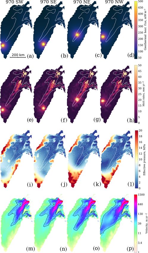
842                                                     S. Smith-Johnsen et al.: Geothermal heat flux at the onset of NEGIS

the ice stream. Beyer et al. (2018) used the basal melt rates      Table 1. Definitions and values of variables in the subglacial hy-
from the model by Aschwanden et al. (2016) in a more so-           drology model.
phisticated hydrology model to reproduce NEGIS in the Ice
Sheet System Model (ISSM). They capture the high velocity                Description                      Unit     Value
flow of the outlets well, but the representation of the transi-          Effective pressure               Pa
tion areas outside of the main trunk are more diffuse com-               Compressibility of water         Pa−1     5.04 × 10⁻¹⁰
pared to the observed values. These studies illustrate how               Leakage factor                   m        1 × 10⁻⁹
we are getting closer to reproducing present-day NEGIS in                Inefficient compressibility      Pa−1     1 × 10⁻⁸
ice sheet models. However, the characteristic clearly defined            Inefficient porosity                      0.4
shear margins, and high velocities upstream at the onset of              Inefficient thickness            m        20
the ice stream are still lacking.                                        Inefficient transmissivity       m2 s−1   0.002
   To understand why high upstream velocities are not re-                Efficient compressibility        Pa−1     1 × 10⁻⁸
produced in models, one must look into how the ice stream                Efficient porosity                        0.4
is initiated. The origin of NEGIS has been explained by a                Efficient initial thickness      m        0.005
geothermal heat flux (GHF) anomaly left behind by the pas-               Efficient collapsing thickness   m        8 × 10⁻⁵
sage of the Icelandic plume (Fahnestock et al., 2001; Ro-                Efficient maximal thickness      m        5
gozhina et al., 2016; Martos et al., 2018; Alley et al., 2019).          Efficient conductivity           m2 s−1   25
Interpretation of radar data points to unusually high basal
melt rates at the head of the ice stream, corresponding to an
exceptionally high GHF of 970 mW m−2 (Fahnestock et al.,           2     Methods
2001; Macgregor et al., 2016; Alley et al., 2019; Keisling
et al., 2014). A local increase in GHF intensifies basal wa-       2.1    Ice flow model
ter production and potentially enhances basal sliding. Un-
                                                                   To simulate the NEGIS ice flow, we apply the model con-
fortunately, GHF maps for Greenland display a large spread
                                                                   figuration from Schlegel et al. (2013, 2015) further devel-
of values (Rogozhina et al., 2012; Shapiro and Ritzwoller,
                                                                   oped and coupled to a subglacial hydrology model by Smith-
2004; Fox Maule et al., 2009; Martos et al., 2018; Rogozhina
                                                                   Johnsen et al. (2019). We use the Ice Sheet System Model
et al., 2016; Greve, 2019). These large uncertainties in the
                                                                   (Larour et al., 2012), a 3D thermomechanical ice flow model,
estimates of the GHF have been shown to dominate the un-
                                                                   and explicitly represent the effect of high melt rates on sub-
certainty on the ice flux in this region (Smith-Johnsen et al.,
                                                                   glacial hydrology (de Fleurian et al., 2014, 2016), which pro-
2019). In addition, the GHF maps are coarse and may not
                                                                   vides the effective pressure (N, the difference between ice
capture local anomalies like the one suggested to exist at the
                                                                   overburden pressure and water pressure at the bed) that con-
head of NEGIS (Fahnestock et al., 2001; Macgregor et al.,
                                                                   trols basal sliding through a linear friction law (Cuffey and
2016; Alley et al., 2019). Accurately capturing such a fea-
                                                                   Paterson, 2010):
ture and explicitly representing the effect of high melt rates
on basal sliding are key to reproduce the distinct velocity pat-   τb = −α 2 Nv b ,                                               (1)
tern of NEGIS in ice sheet models.
   Here, we study the impact of the presence and intensity of      where τb is the basal drag, α the basal friction coefficient
a mantle plume, at the head of NEGIS on the ice flow struc-        and v b the basal velocity. The hydrology model takes the
ture. We do not suggest the presence of a mantle plume, but        basal melt rates as input and computes the effective pres-
rather use an existing mantle plume model to generate fea-         sure. Nodes with no basal melt are given an effective pressure
sible GHF scenarios in the model sensitivity study. We use         equal to the ice overburden pressure. The hydrology model
a sophisticated hydrology model (de Fleurian et al., 2014,         consists of two porous sediment layers, representing the in-
2016) coupled to ice dynamics in the Ice Sheet System Model        efficient and efficient drainage system. The efficient drainage
(ISSM; Larour et al., 2012) to capture the influence of en-        system is activated when N reaches zero and may be deacti-
hanced basal melt on ice dynamics. We first describe the           vated as the water is evacuated and N increases again. Def-
models and different plume experiments. Finally, we present        initions and values of variables in the subglacial hydrology
and discuss resulting basal conditions and surface velocities      model are given in Table 1. The hydrology model and its im-
corresponding to the various plume configurations.                 plementation in ISSM are described in detail in de Fleurian
                                                                   et al. (2014, 2016).
                                                                      For the thermal model we rely on the enthalpy formu-
                                                                   lation by Aschwanden et al. (2012), implemented in ISSM
                                                                   (Seroussi et al., 2013) with surface temperatures from Et-
                                                                   tema et al. (2009) and GHF from Fox Maule et al. (2009).
                                                                   In addition we use a mantle plume module in ISSM to create
                                                                   elevated GHF anomalies (Seroussi et al., 2017). Ice is treated

The Cryosphere, 14, 841–854, 2020                                                          www.the-cryosphere.net/14/841/2020/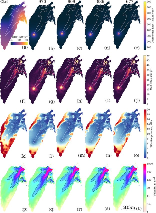
S. Smith-Johnsen et al.: Geothermal heat flux at the onset of NEGIS                                                            843

as a purely viscous incompressible material (Cuffey and Pa-        for the NEGIS region shows a pattern inversely correlated
terson, 2010), with viscosity, µ, defined as                       with bed elevation (Cooper et al., 2019). This relation might
                                                                   however not hold on smaller scales under the NEGIS trunk
       B
µ=      n−1
              ,                                             (2)    where the till distribution is independent of the bed geometry
     2˙e n                                                        (Christianson et al., 2014). Some alternatives to using this
                                                                   parameterisation are given in the discussion section of this
where B is the temperature-dependent ice hardness varying          paper.
with depth, n is Glen’s flow law exponent and ˙e is the effec-
tive strain rate.
   Basal topography is from BedMachine (Morlighem et al.,          2.2   Experiments
2014) (Fig. 1a) and we apply submarine melt rates under
the floating ice (Rignot et al., 2001). For the stress balance     In order to capture the high upstream velocity of NEGIS,
equation, we use a 3D higher-order approximation (Pattyn,          we alter the GHF by simulating a mantle plume close to the
2003). Our model domain consists of 9974 horizontal ele-           head of the ice stream, at the onset of fast flow (Seroussi
ments, ranging from 1 km in areas with high velocity gra-          et al., 2017). The mantle plume module in ISSM computes
dients to a maximum of 15 km at the ice divide (Fig. 1b).          the GHF, given the plume parameters in Table 2. To disen-
We use linear P1 elements to solve the stress balance equa-        tangle the effect of the mantle plume we run a control simu-
tions and quadratic P2 elements for the thermal analysis, in       lation without a mantle plume, using only the GHF from Fox
order to capture sharp temperature gradients, despite using        Maule et al. (2009). This GHF map ranges from 40 mW m−2
only five layers (Cuzzone et al., 2018).                           in the northwest to 77 mW m−2 in the northeast below the
   We aim to represent the observed NEGIS velocity pattern         Storstrømmen outlet, with an average value of 54 mW m−2 .
in an ice sheet model without inverting for the basal fric-           In our main experiment, plume970, the plume parameters
tion coefficient. However, to initialise the hydrology model,      were chosen to generate a GHF anomaly coherent with the
we do simulate the present-day ice stream by inferring basal       magnitude of the GHF anomaly hypothesised by Fahnestock
friction from present-day velocities (Fig. 1b). The basal melt     et al. (2001). The resulting GHF anomaly is ∼ 50 km in diam-
rates from this simulation are used to initialise the subglacial   eter with a maximum GHF value of 970 mW m−2 (Table 3),
hydrology model, which we run for 150 years in order to            and we position it directly underneath the EGRIP deep ice
reach an equilibrium in terms of water pressure. The resulting     core drilling site (Fig. 1c).
effective pressure field computed by the hydrology model,             To determine the minimum GHF needed to initiate the
N, is used in the friction law (Eq. 1) and kept constant in        onset of NEGIS close to the ice divide, we compute three
time. Finally, we run a 4 kyr simulation with the basal con-       alternative plume configurations with lower intensity. We
dition generated by the hydrology model to provide steady-         obtain the lower GHF by decreasing the bottom plume
state surface velocities. Note that we do not use the friction     depth parameter to 4500, 4000 and 3000 km for simula-
coefficient, α, from the inversion in the forward ice flow sim-    tions plume909, plume836 and plume677, respectively (Ta-
ulation, as it is only used to initialise the subglacial hydrol-   ble 3). Additionally, we compute four plume configura-
ogy model.                                                         tions where we change the position of the plume. We move
   Previous modelling studies lack sharp velocity gradients        plume970 75 km to the southwest, southeast, northeast and
defining NEGIS (Aschwanden et al., 2016; Beyer et al.,             northwest in the plume970SW, plume970SE, plume970NE
2018). To capture this we let the basal friction coefficient,      and plume970NW experiments, respectively (Table 3). To in-
α, depend linearly on the bed elevation using the following        vestigate the influence of the area of the mantle plume, we
equation:                                                          compute four plume configurations with larger area, com-
α = min(max(1, 0.13 × bed + 100), 250),                     (3)    pensated for by a smaller heat flux. To obtain this we increase
                                                                   the plume radius to values of 100–300 km, and we decrease
where 100 (m s−1 )1/2 is the mean value of the inversion alpha     the bottom plume depth to values of 2000–3000 km, result-
used in Smith-Johnsen et al. (2019), and we cap the values         ing in the experiments plume494, plume594, plume775 and
between 1 and 250 (m s−1 )1/2 . The factor 0.13 is tuned to ap-    plume792 (Table 3).
proximately match the observed velocities at the grounding            Finally, to investigate the influence of our friction coeffi-
line of 79N. The resulting friction coefficient, α, is shown in    cient distribution, we run three additional simulations. First,
Fig. 1c. We argue that low-lying topography will have more         we run a simulation without modelled effective pressure,
marine sediments, and thus a softer and less resistive bed,        but instead using effective pressure approximated to hydro-
allowing high velocities of the outlet glaciers. A similar ap-     static pressure, commonly used in ISSM (noHydro, Table 3).
proach with basal shear stress defined as a function of bed el-    Then we run two simulations with a uniform friction of
evation was previously used by Åkesson et al. (2018) and by        α = 90 (m s−1 )1/2 : one without a plume (Ctrl-uni, Table 3)
Aschwanden et al. (2016). Our simple friction relationship         and one with the 970 mW m−2 plume (plume970-uni, Ta-
is supported by observations, as bed topography roughness          ble 3).

www.the-cryosphere.net/14/841/2020/                                                        The Cryosphere, 14, 841–854, 2020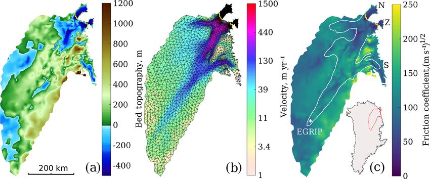
844                                                         S. Smith-Johnsen et al.: Geothermal heat flux at the onset of NEGIS

Figure 1. (a) Bed topography from BedMachine (Morlighem et al., 2014) interpolated onto the model mesh; (b) InSAR-derived surface
velocities (Rignot and Mouginot, 2012) and anisotropic model mesh refined in areas with high velocity gradients; (c) friction coefficient as a
linear function of bed topography (Eq. 3) used in Eq. (1). The white contour shows the area of the NEGIS with observed surface velocity of
50 m yr−1 and the star shows the position of the East Greenland Ice-Core Project (EGRIP). N, Z and S indicate the outlets of the ice stream:
79N, Zachariæ and Storstrømmen, respectively. The yellow line in all panels represents the grounding line, and the inset map in the lower
right corner shows Greenland with the model domain outlined in red.

Table 2. Mantle plume parameter overview for the plume experiments.

                     Parameter               Description                                        Value           Unit
                     Mantleconductivity      mantle heat conductivity                           2.5             W m−3
                     Nusselt                 Nusselt number, ratio of mantle to plume           500 000
                     Dtbg                    background temperature gradient                    0.013           ◦ m−1
                     Plumeradius             radius of the mantle plume                         varying         m
                     Topplumedepth           depth of the mantle plume top below the crust      5000            m
                     Bottomplumedepth        depth of the mantle plume base below the crust     varying         km
                     Crustthickness          thickness of the crust                             1               m
                     Uppercrustthickness     thickness of the upper crust                       1               m
                     Uppercrustheat          volumic heat of the upper crust                    1.33 × 10⁻⁶     W m−3
                     Lowercrustheat          volumic heat of the lower crust                    2.7 × 10⁻⁷      W m−3

3   Results                                                              coincide with low bed elevation in the main trunk, 100 km
                                                                         upstream of the grounding line.
                                                                            The resulting velocity field for the control simulation cap-
                                                                         tures the main features of NEGIS: the three outlets with high
In the control simulation we use the GHF from Fox Maule
                                                                         velocities across the grounding lines and sharp shear margins
et al. (2009) (Fig. 2a), and the corresponding basal melt rates
                                                                         (Fig. 2p). The northern branch feeding into 79N is slower and
are shown in Fig. 2f. Melt rates at the head of the ice stream
                                                                         less defined than in the observed velocities, and the velocities
(at EGRIP) are 1–2 mm yr−1 , and the highest basal melt rates
                                                                         of Storstrømmen are also slower than observed. Velocities of
(600 mm yr−1 ) occur at the grounding line of Zachariæ, with
                                                                         the floating tongues of 79N and Zachariæ are not well repre-
surface velocities reaching 1500 m yr−1 . Friction is the dom-
                                                                         sented, and floating shelves are not shown here. The western
inating heat source in the fast-flowing regions, and melt rates
                                                                         branch, feeding into the main trunk of NEGIS, shows a more
thus increase with increasing velocities towards the ground-
                                                                         diffuse pattern with higher velocities than observed.
ing line. Low melt rates in regions with high velocity are
                                                                            To evaluate how well the model simulations reproduce
due to low-lying bed topography causing low basal drag and
                                                                         the observed velocity pattern, we plot the 50 m yr−1 veloc-
hence less frictional heat. The effective pressure for the con-
                                                                         ity contour (black contour in Fig. 2), and we compare how
trol experiment is shown in Fig. 2k, and the values increase
                                                                         far upstream this contour reaches (in kilometres from the ice
upstream toward the ice divide as ice thickness increases and
                                                                         divide) relative to the observed velocity (white contour in
basal melt decreases. The lowest values of effective pressure

The Cryosphere, 14, 841–854, 2020                                                                www.the-cryosphere.net/14/841/2020/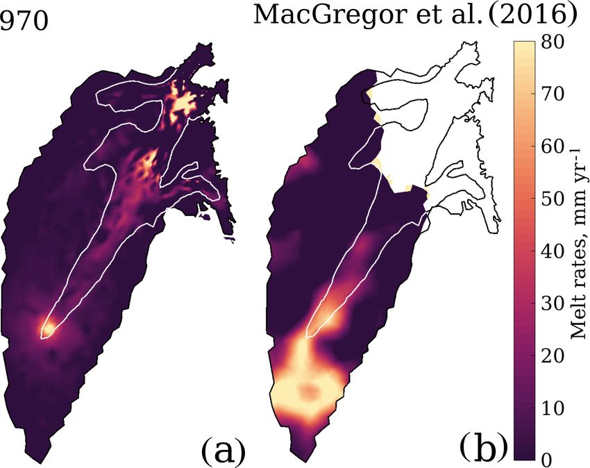
S. Smith-Johnsen et al.: Geothermal heat flux at the onset of NEGIS                                                           845

Table 3. Overview of mantle plume parameters, modelled GHF and friction parameters.

          Simulation      Position    Radius (km)    Depth (km)    Max GHF (mW m−2 )      α ((m s−1 )1/2 )   N (MPa)
          Control         no plume       no plume      no plume                no plume   varying            modelled
          Plume970        centre               50          5000                     970   varying            modelled
          Plume677        centre               50          3000                     677   varying            modelled
          Plume836        centre               50          4000                     836   varying            modelled
          Plume909        centre               50          4500                     909   varying            modelled
          Plume970SW      SW                   50          5000                     970   varying            modelled
          Plume970SE      SE                   50          5000                     970   varying            modelled
          Plume970NE      NE                   50          5000                     970   varying            modelled
          Plume970NW      NW                   50          5000                     970   varying            modelled
          Plume494        centre              300          3000                     494   varying            modelled
          Plume594        centre              200          2500                     594   varying            modelled
          Plume775        centre              100          2000                     775   varying            modelled
          Plume792        centre              200          3000                     792   varying            modelled
          NoHydro         no plume       no plume      no plume                no plume   varying            approximated
          Ctrl-uni        no plume       no plume      no plume                no plume   90                 modelled
          Plume970-uni    centre               50          5000                     970   90                 modelled

Fig. 2). The modelled velocity contour in the control sim-             To determine whether a lower GHF may induce a sim-
ulation reaches 305 km from the ice divide (Fig. 2p) and            ilar high-velocity pattern, we run three simulations with a
thus further downstream than the observed velocity (120 km,         less intense mantle plume. Figure 2c–e show the GHF values
Fig. 2a, f, k). The control simulation does not capture the         computed by increasing the plume depth to 3000, 4000 and
characteristics of NEGIS, with high upstream velocities close       4500 km, respectively, obtaining maximum basal melt rates
to the ice divide.                                                  of ∼ 70 (Fig. 2j), ∼ 85 (Fig. 2i) and ∼ 95 mm yr−1 (Fig. 2h).
   To capture the upstream velocities, we enhance the GHF           The modelled effective pressure for the three plumes
locally at the onset of the ice stream in the plume970 simu-        (Fig. 2m–o) results in slower velocities than plume970, with
lation to reach the maximum magnitude proposed by Fahne-            50 m yr−1 velocity contours reaching 253, 245 and 210 km
stock et al. (2001). The addition of the mantle plume results       from the ice divide, respectively (Fig. 2r–t). This shows that
in high GHF, with values up to 970 mW m−2 , rapidly de-             GHF values of 677, 836 and 909 mW m−2 produce weaker
creasing to the values used in the control simulation (Fig. 2b)     ice stream signatures than observed and, given our model
within a radius of less than 100 km. High geothermal heat           set-up, are not sufficient to induce the upstream fast flow of
leads to high basal melt rates, with ∼ 100 mm yr−1 above            NEGIS.
the plume (Fig. 2g), compared to 1–2 mm yr−1 in the con-               To investigate the sensitivity of the position of the plume
trol experiment. The increase in basal melt rates causes a re-      in plume970, we moved the plume 75 km to the southwest,
duction in effective pressure to 1.2 MPa directly above the         southeast, northeast and northwest (Fig. 3). The computed
plume, resulting in a local floatation fraction (ratio of wa-       GHF distribution is shown in Fig. 3a–d and the basal melt
ter pressure over overburden pressure) of 0.95. The result-         rates are of the same magnitude as in plume970. The com-
ing velocity field in the plume970 experiment is similar to         puted effective pressures for the southwest and southeast
the control experiment, except for the higher velocities sim-       (plume970SW and plume970SE, Fig. 3i, j) have minimum
ulated at the head of the ice stream. In the plume970 sim-          values of 3.2 and 2.9 MPa above the plume, which are not
ulation the 50 m yr−1 velocity contour reaches 131 km from          sufficient to initiate fast flow (Fig. 3m, n). When the plume
the ice divide (black contour Fig. 2q), which is close to the       is located further downstream, the effective pressure reaches
observed 120 km. However, the spatial pattern upstream is           lower values (Fig. 3k, l) and the ice stream flows faster
more diffuse and the ice stream is wider than observed. The         than in plume970 (Fig. 3o, p), however, with the 50 m yr−1
Storstrømmen outlet shows higher velocities relative to the         contour only reaching 204 km from the ice divide. The
control simulation, but still lower than observed. The 79N          plume970NE induces the fastest flow, and the plume970NW
and Zachariæ outlets, on the other hand, display higher ve-         creates an interesting double-branched ice stream starting
locities than observed. Overall, with this approach, we cap-        from the ice divide. The experiments in Fig. 3 indicate that
ture most of the characteristics of NEGIS, although the ice         the elevated heat required to initiate the NEGIS in our model
stream is more diffuse and displays velocities slightly higher      must be located close to EGRIP.
than the observations.                                                 To determine whether a lower GHF value over a larger
                                                                    area could induce high upstream velocities, we investigate

www.the-cryosphere.net/14/841/2020/                                                        The Cryosphere, 14, 841–854, 2020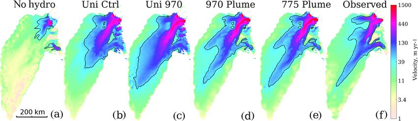
846                                                        S. Smith-Johnsen et al.: Geothermal heat flux at the onset of NEGIS

Figure 2. Model results for the control simulation and the plume677, plume836, plume909 and plume970 simulations. Panels (a–e) show
the modelled GHF (note the different colour scale for the control simulation) and (f–j) show the corresponding basal melt rates, forcing the
hydrology model which computes the corresponding effective pressure (k–o) and finally the resulting surface velocity (p–t). White lines
show the 50 m yr−1 observed velocity contour, and black lines show the 50 m yr−1 modelled velocity contour.

The Cryosphere, 14, 841–854, 2020                                                              www.the-cryosphere.net/14/841/2020/
S. Smith-Johnsen et al.: Geothermal heat flux at the onset of NEGIS                                                                 847

Figure 3. Model results from the sensitivity simulations investigating the position of the mantle plume by moving the plume970 75 km. The
first column shows results from plume970SW, with a plume 75 km to the southwest; the second column represents the 970 SE plume; the
third column represents plume970NE; and the last column is plume970NW. Panels (a–d) show the GHF, (e–h) the resulting basal melt rates,
(i–l) the computed effective pressure and (m–p) the modelled surface velocity. White lines show the 50 m yr−1 observed velocity contour,
and black lines show the 50 m yr−1 modelled velocity contour.

www.the-cryosphere.net/14/841/2020/                                                             The Cryosphere, 14, 841–854, 2020
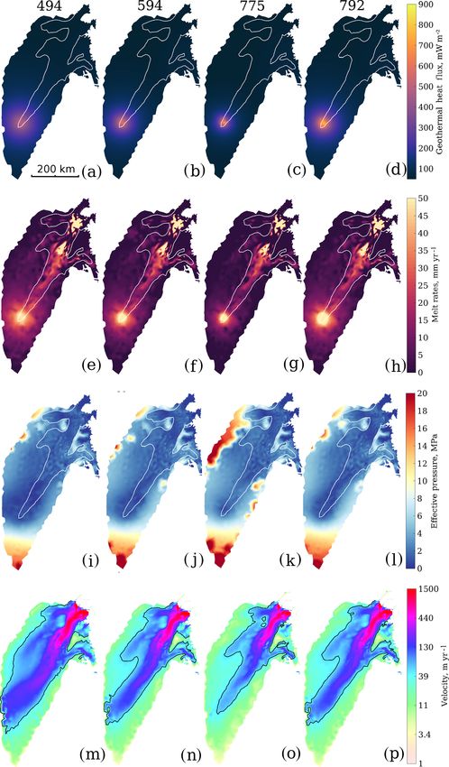
848                                                      S. Smith-Johnsen et al.: Geothermal heat flux at the onset of NEGIS

Figure 4. Model results from the sensitivity simulations investigating a reduced magnitude and increased size of the mantle plume. The
first column shows results from the 494 plume with a 300 km radius at 3000 km depth, the second column represents the 594 plume with a
200 km radius and 2500 km depth, the third column represents the 775 plume with a 100 km radius and 2000 km depth, and the last column
represents plume 792 with a 200 km radius and 3000 km depth. Panels (a–d) show the GHF, (e–h) the resulting basal melt rates, (i–l) the
computed effective pressure and (m–p) the modelled surface velocity. White lines show the 50 m yr−1 observed velocity contour, and black
lines show the 50 m yr−1 modelled velocity contour.

The Cryosphere, 14, 841–854, 2020                                                            www.the-cryosphere.net/14/841/2020/
S. Smith-Johnsen et al.: Geothermal heat flux at the onset of NEGIS                                                                      849

Figure 5. Surface velocity results from the noHydro simulation (a) with effective pressure approximated to the hydrostatic pressure assuming
direct connection to the ocean, commonly used in ISSM. Uni control (b) and plume970-uni experiments (c) use a uniform friction coefficient
α set equal to 90 (ms−1 )1/2 . Corresponding GHF, basal melt rates and effective pressure are the same as the control simulation and plume970,
shown in Fig. 2. For reference we include (d) and (e), respectively, showing the plume970 and plume775 simulations (same as Figs. 2q,
and 4o), and (f) showing the observed surface velocities interpolated onto the model mesh. Black lines show the 50 m yr−1 velocity contour.

the influence of four weaker plumes with larger plume radii              4    Discussion
(Fig. 4). The weakest but most extensive plume (plume494,
Fig. 4a) produces basal melt rates of a maximum of
51 mm yr−1 (Fig. 4e), resulting in a large area of low effec-            Most of the spatial velocity pattern of NEGIS is represented
tive pressure (minimum 0.2 MPa; Fig. 4i). The corresponding              in our control run, apart from the upstream one-third of the
surface velocity for the plume494 displays a faster and wider            main trunk. This indicates that the downstream area of the
ice stream (Fig. 4m) relative to the observations. Plume594              NEGIS catchment is largely controlled by topography, while
gives basal melt rates of 60 mm yr−1 (Fig. 4f) and the ice               the upstream area is controlled by its basal conditions, which
stream becomes wide, reaching all the way to the ice di-                 is in agreement with Keisling et al. (2014). The control sim-
vide (Fig. 4n). Plume775 is twice the size of plume970                   ulation captures the main outlets and the observed snake-
(Fig. 4c), and with melt rates of ∼ 75 mm yr−1 over a larger             shaped velocity pattern of the trunk. High velocities coincide
area (Fig. 4g) the velocity of the ice stream (Fig. 4o) is               with low-lying bed elevation. However, we do not capture
similar to plume970. However, the 50 m yr−1 velocity con-                the high velocity of Storstrømmen, or the floating tongues of
tour reaches too close to the ice divide and the ice stream is           the Zachariæ and 79North outlets. This could be caused by
wider than the observed one. Plume792 produces melt rates                the simple friction coefficient approach not being represen-
of ∼ 75 mm yr−1 (Fig. 4d), resulting in velocities similar to            tative of these areas, where basal properties display a more
those of plume594 (Fig. 4p). This shows that plumes with                 complex pattern.
a restricted extent, ∼ 50 km × 50 km, produce model results                 We performed experiments with various mantle plume
more consistent with the observed flow behaviour in the up-              configurations introduced at the head of NEGIS to assess
stream reaches of NEGIS.                                                 if the presence of an anomalously high GHF can explain
   Finally, we investigate the influence of varying the pa-              the pattern of ice flow of this region. The different plume
rameters in the friction law (Eq. 1), presented in Fig. 5.               configurations vary in intensity, position and extent. In the
The noHydro simulation with an effective pressure approx-                control simulation we use present-day surface velocity and
imated to the hydrostatic pressure shows very little resem-              GHF from Fox Maule et al. (2009). Without the presence of
blance to the observed NEGIS (Fig. 5a), with too slow ve-                a plume, the GHF does not reach more than 54 mW m−2 and
locities. The simulation with a uniform friction coefficient             leads to underestimating velocities in the upstream part of
and no mantle plume captures the main feature of NEGIS                   the catchment. These low values of GHF are not sufficient to
(Ctrl-uni, Fig. 5b): with a main trunk, the northern branch              initiate the onset of NEGIS close to the ice divide. By testing
and three outlets, with the fastest flow in Zachariæ. How-               with four mantle plume configurations of increasing inten-
ever, the velocity pattern is more diffuse than the observed             sity (Fig. 2), we find that the GHF (GHF) needed to induce
pattern (Fig. 5e). The high upstream velocities are better cap-          the observed upstream velocity of NEGIS in our model is
tured in the simulation with plume970 and a uniform friction             ∼ 970 mW m−2 .
(plume970-uni, Fig. 5c). For plume970-uni, high velocities                  A GHF of 970 mW m−2 is consistent with the maximum
reach slightly closer to the ice divide than plume970, but the           value presented in Fahnestock et al. (2001) and Keisling et al.
velocities of the main trunk are less confined than in experi-           (2014) for regions in proximity to EGRIP, where plume970
ment plume970 (Fig. 5d) and the observations (Fig. 5f).                  is located. It also compares well to the anomaly modelled
                                                                         by Macgregor et al. (2016) in the trunk of NEGIS but does
                                                                         not include the high GHF that they find upstream. These
                                                                         GHF values are imposed based on basal melt estimates from

www.the-cryosphere.net/14/841/2020/                                                                 The Cryosphere, 14, 841–854, 2020
850 S. Smith-Johnsen et al.: Geothermal heat flux at the onset of NEGIS
a large discrepancy between the necessary GHF to produce
this melt and the GHF estimates for Greenland.
To explain the high GHF value of 970 mW m−2 , we need
to investigate processes that may locally elevate the GHF.
Alley et al. (2019) and Stevens et al. (2016) explained high
GHF in this region by the passing of the Iceland plume,
leaving behind partly molten rock that may have migrated
up in response to glacial–interglacial cycles, as the crust is
loaded and unloaded. A study showed that glacial rebound
may have caused young intraplate volcanism in Greenland,
despite the old age of the tectonic plate and no mantle
plume present (Uenzelmann-Neben et al., 2012). The plume
passage could have lead to shallow magma emplacements,
which may feed hydrothermal systems, causing hot fluid per-
colation that enhances high heat transport to the base of the
Figure 6. Comparison of the basal melt rates computed for the ice sheet (Stevens et al., 2016; Alley et al., 2019; Mordret,
plume970 experiment (a) and the gridded basal melt rate estimates 2018). It is important to note that the term GHF is defined
of Macgregor et al. (2016) interpolated onto our model mesh (b). as the heat flux from the Earth’s interior as a purely conduc-
White lines show the observed 50 m yr−1 velocity contour. tive heat transfer. Hence, the 970 mW m−2 heat flux can not
be explained by GHF alone but rather also with surface heat
flow from locally elevated GHF due to advective heat transfer
radar internal stratigraphy. Our modelled basal melt rates from the processes mentioned above (Artemieva, 2019).
(∼ 100 mm yr−1 ) are thus consistent with their proposed Comparing the velocity field in the plume970 experiment
values. By directly comparing the basal melt rates of our to previous studies without inversion shows that combin-
plume970 experiment to the basal melt rate estimates from ing a basal hydrology model with an elevated GHF at the
Macgregor et al. (2016) in Fig. 6, it can be seen that our head of NEGIS captures the observed high, confined, up-
plume produces a basal melt pattern that matches the posi- stream velocities of the NEGIS. The simulations in Goelzer
tion, extent and values of the northeastern branch of their et al. (2018) show that the ice flow models capturing the up-
anomaly. The sensitivity simulations in Fig. 3m, n show that stream onset of NEGIS all rely on inversions to initialise
more than 970 mW m−2 is needed to initiate high velocity, the basal drag in the simulations (Elmer/Ice, ISSM, BISI-
when the plume is located further upstream in a region with CLES, GRISLI and f.Etish). The models without inversion
thicker ice relative to downstream. This suggests that the area underestimate the velocities in the upper part of the NEGIS
of high basal melt estimated by Macgregor et al. (2016) in catchment and lack the sharp velocity gradients. Aschwan-
the trunk of NEGIS is probably more consequential than the den et al. (2016) simulated the high upstream velocity of
larger melt anomaly that they modelled closer to the divide. NEGIS without inverting for basal conditions in Parallel Ice
The GHF at the head of NEGIS is suggested to be high Sheet Model (PISM), but their simulation lacks the clearly
due to lithospheric thinning as a result of the Iceland plume defined main trunk and underestimates the high upstream
passage (Rogozhina et al., 2016; Martos et al., 2018). How- velocity. Beyer et al. (2018) further improved the simula-
ever, 970 mW m−2 is an extremely high GHF value, 10 to 20 tion by using a subglacial hydrology model to compute ef-
times higher than the values suggested by GHF models for fective pressure, which allowed higher velocities in the out-
Greenland (Shapiro and Ritzwoller, 2004; Fox Maule et al., lets. However, high upstream velocities are still lacking, sim-
2009; Martos et al., 2018; Rogozhina et al., 2016). Greve ilar to our control simulation. The last two studies used GHF
(2019) derived GHF values for five deep ice core boreholes in from Shapiro and Ritzwoller (2004), which proposed slightly
Greenland, using the SICOPOLIS model (SImulation COde lower values at the head of NEGIS compared to the values of
for POLythermal Ice Sheets; http://www.sicopolis.net/, last Fox Maule et al. (2009) used in our study.
access: 4 March 2020), such that the simulated and observed Beyer et al. (2018) used the same friction law as we use
basal temperatures match. This resulted in a local elevated in ISSM, but with a uniform friction coefficient. We tested
GHF anomaly around NGRIP of 135 mW m−2 , located at the a uniform friction coefficient, which led to a more diffuse
ice divide ∼ 150 km away from the head of NEGIS. Our GHF ice stream (Fig. 5b, c), but with more confined outlets com-
anomaly has a magnitude 7 times higher than that of Greve pared to the Beyer et al. (2018) study. The difference can be
(2019) and 3 times as high as the highest current GHF ob- explained by different basal melt rates used as input and dif-
servations in Greenland (Rysgaard et al., 2018). In summary, ferent hydrology models. In order to capture sharp gradients
plume970 produces a basal melt pattern with magnitude and in the velocity field, we find it important that the areas with-
extent in line with previous estimates from the radar data out any basal melt have effective pressure equal to the ice
for the region within the 50 m a−1 isoline; however there is overburden pressure.
The Cryosphere, 14, 841–854, 2020 www.the-cryosphere.net/14/841/2020/S. Smith-Johnsen et al.: Geothermal heat flux at the onset of NEGIS 851 We invert for basal friction to get the basal melt rates and hence overestimate the lateral drag. Refining the mesh that are used to initialise the subglacial hydrology model, and inducing damage softening of the ice in the shear mar- and the model is then free to evolve. We do not use the in- gins (Bondzio et al., 2017) would decrease the lateral drag. In verted friction in the forward ice flow simulation; instead this case, the observed high upstream velocity of NEGIS may we use the simple friction coefficient from Eq. (3). To in- have been reproduced with higher basal drag and hence lower vestigate whether the modelled velocity pattern is caused GHF. The underestimation of modelled ice softness may also by the effective pressure distribution or the friction coeffi- explain why our modelled upstream velocity field is wider cient, we run the simulation noHydro, where the effective and more diffuse than the observed field. pressure is approximated to the hydrostatic pressure, com- In the simulations where we investigate the influence of an monly used in ISSM. The modelled velocity pattern (Fig. 5a) increased plume radius (Fig. 4), we show that lower values does not resemble the observed pattern, and we conclude of GHF can induce even faster flow, when the plume is more that including the subglacial hydrology model is responsible extensive (Fig. 4). However, with a larger mantle plume the for the improved velocity pattern in the control simulation ice stream becomes wider and does not match the observed and plume970. By using our friction coefficient distribution, velocity of NEGIS (Fig. 5e). The basal melt pattern of Mac- combined with initialising with present-day basal melt from gregor et al. (2016) in Fig. 6 consists of two melt anomalies velocity observations, both the control and plume970 exper- near EGRIP. It would be interesting to investigate the veloc- iments display velocity patterns similar to the observations ity response of two weaker elevated GHF anomalies closely (Fig. 5d, e). located. There is also room for improvement of the model in The middle western branch of the ice stream displays too the treatment of the shear margin or the use of a non-linear high velocity in both the control and plume970 experiments, friction law (Gagliardini et al., 2007; Schoof, 2005). Both correlating with low-lying bed elevation (Fig. 1). Too high those improvements would lead to sharper transition from velocities in this region were also modelled by Aschwan- slow to fast velocities and might allow a plume with a larger den et al. (2016) using PISM and a similar bed-elevation- radius. dependent friction law. When performing additional simula- We parameterise the friction coefficient with a simplified tions with the GHF values from Martos et al. (2018), this estimate linearly dependent on the bed elevation. In other branch becomes more pronounced in velocity (not shown studies this coefficient is inverted for by matching observed here). This may indicate that the GHF values in this region of surface velocity, producing low values in the main trunk of Greenland are even lower than those in Martos et al. (2018) NEGIS (Smith-Johnsen et al., 2019). By lowering the fric- and Fox Maule et al. (2009), and the glacier base is frozen tion in the main trunk, we may reproduce fast flow with a to the ground. This region is recognised as “uncertain” in the lower GHF value. However, this would make the friction co- synthesis of Greenland’s basal thermal regime by Macgregor efficient relate to the velocity, which we are trying to avoid. et al. (2016). Other explanations for too high velocities in The bed topography used is from BedMachine (Morlighem this branch may be a higher bed roughness, errors in the bed et al., 2014), so datasets used to create this map impact the topography or “sticky spots”. choice of friction. A uniform lowering of the friction coef- Given the model configuration, an exceptionally high heat ficient, also outside the trunk, would increase velocities all flux of 970 mW m−2 is needed to reproduce NEGIS. We ac- over the domain; hence we would lose the sharp velocity knowledge that this value may be overestimated due to uncer- gradients and overestimate the outlet velocity even further. tainties and assumptions in our model set-up, and we discuss Additionally, the modelled ice surface in the control exper- these in the following sections. We use a simple friction law iment is lower than the observed ice surface (Scambos and linearly dependent on effective pressure, and we are aware Haran, 2002), and a uniform reduction of friction will en- that the results are likely to change with a different choice hance this mismatch. We do not observe a local depression in of friction law. For example, in the friction law used in the the surface topography above the 970 mW m−2 plume, which MISMIP+ experiments (Asay-Davis et al., 2016; Tsai et al., agrees with the observed ice surface for the region (Scambos 2015), effective pressure is included only where the coulomb and Haran, 2002). criterion is met, normally a few kilometres upstream of the Hydrology parameters are unfortunately highly uncertain, grounding line. This may result in a smaller dynamic re- and different choices would lead to a more or less responsive sponse from the mantle plume in the slow upstream regions hydrological system and hence possibly a lower GHF value of NEGIS. However, the use of a non-linear friction law may to sustain the fast flow. However, we have a rather low trans- enhance the sensitivity of the ice dynamics to effective pres- missivity of the inefficient drainage system, resulting in low sure, also upstream, as we compute low effective pressure efficiency in water evacuation, causing our system to be sen- above the plume. This implies that the use of a non-linear sitive to an increase in water input. If the transmissivity was friction law may result in a lower GHF needed to sustain lowered further, the efficient drainage system is likely to acti- NEGIS in a model. vate in the GHF anomaly region, lowering the water pressure By using a coarse model mesh we may underestimate the and becoming less sensitive to increased water input. For this softening occurring due to strain heating in the shear margins reason, we do not expect that a different hydrology configu- www.the-cryosphere.net/14/841/2020/ The Cryosphere, 14, 841–854, 2020
852                                                         S. Smith-Johnsen et al.: Geothermal heat flux at the onset of NEGIS

ration would reproduce NEGIS with a lower heat flux. In ad-            Author contributions. SSJ designed the study with help from BdF
dition, the subglacial hydrology is only one-way coupled to            and KHN. SSJ ran the simulations. NS helped greatly in set up
ice dynamics, so we do not capture the positive feedback ex-           the ice flow model, BdF helped set up the hydrology model, and
pected with higher velocities leading to more melt, and lower          HS helped setting up the mantle Plume model. SSJ wrote the
effective pressure, giving even higher velocities. With a more         manuscript with substantial contributions from all co-authors. The
                                                                       research related to the paper was discussed by all co-authors.
responsive and fully coupled system, one might be able to re-
produce NEGIS with lower heat flux.
   With a simple bed-elevation-dependent friction and hy-
                                                                       Competing interests. The authors declare that they have no conflict
drology model forced by melt rates from GHF, we capture
                                                                       of interest.
the overall pattern of NEGIS velocity. This has implications
for studies trying to predict the response of NEGIS to a fu-
ture climatic warming. Basal friction may not remain con-              Acknowledgements. Silje Smith-Johnsen, Basile de Fleurian and
stant in time, and thus we cannot fully rely on inversion as           Kerim Nisancioglu were funded by the Ice2Ice project that has re-
it masks unknown time-varying basal properties. By using               ceived funding from the European Research Council under the Eu-
our approach (with or without the GHF anomaly) one can                 ropean Community’s Seventh Framework Programme (FP7/2007-
capture complex velocity patterns and then invert for the re-          2013)/ERC grant agreement no. 610055. Basile de Fleurian is also
maining basal properties. These may in turn be assumed to be           funded by the SWItchDyn NRC grant (287206). Funding for He-
constant in time, while the subglacial hydrology will evolve           lene Seroussi and Nicole Schlegel was provided by grants from
with a changing climate, accounting for varying basal condi-           the NASA Cryospheric Science and Modeling, Analysis and Pre-
tions. Unfortunately, observations and estimates of GHF and            diction (MAP) programmes. We would like to thank the reviewers
                                                                       Nicholas Holschuh and Signe Hillerup Larsen for greatly improv-
subglacial hydrology are challenged by large uncertainties.
                                                                       ing the manuscript. We would also like to thank Irina Rogozhina
Therefore, it is critical for future observational and modelling
                                                                       and Ralf Greve for good discussions and recommendations.
studies to better constrain the basal conditions of the Green-
land Ice Sheet.
                                                                       Financial support. This research has been supported by the Euro-
                                                                       pean Research Council (ICE2ICE, grant no. 610055) and the Nor-
5   Conclusions
                                                                       wegian Research Council (SWItchDyn, grant no. 287207).
Present-day basal melt rates from GHF maps and frictional
heat are not sufficient to sustain the observed upstream veloc-
                                                                       Review statement. This paper was edited by Nanna Bjørnholt
ities of the Northeast Greenland Ice Stream (NEGIS). The
                                                                       Karlsson and reviewed by Nicholas Holschuh and Signe Hillerup
downstream velocities appear to be driven by topography,               Larsen.
and the spatial pattern is well captured by the subglacial hy-
drology model. Our findings suggest that a local heat flux
anomaly may explain the characteristic high upstream ve-
locity of NEGIS and hence is consistent with previous stud-            References
ies (Fahnestock et al., 2001; Macgregor et al., 2016; Alley
et al., 2019). To reproduce high upstream velocities at the            Åkesson, H., Morlighem, M., Nisancioglu, K., Svendsen, J., and
onset of NEGIS, a sustained basal melt rate of 100 mm yr−1               Mangerud, J.: Atmosphere-driven ice sheet mass loss paced
is needed in a local region close to EGRIP, where observed               by topography: Insights from modelling the south-western
present-day velocities reach 50 m yr−1 . Hence, the minimal              Scandinavian Ice Sheet, Quaternary Sci. Rev., 195, 32–47,
heat flux value needed to initiate the ice stream in our model           https://doi.org/10.1016/j.quascirev.2018.07.004, 2018.
is 970 mW m−2 , as proposed by Fahnestock et al. (2001).               Alley, R. B., Pollard, D., Parizek, B. R., Anandakrishnan, S., Pour-
                                                                         point, M., Stevens, N. T., MacGregor, J., Christianson, K., Muto,
This magnitude is too high to be explained by GHF alone,
                                                                         A., and Holschuh, N.: Possible Role for Tectonics in the Evolv-
and we suggest that processes such as hydrothermal circula-              ing Stability of the Greenland Ice Sheet, J. Geophys. Res.-Earth,
tion may locally elevate the heat flux of the area.                      124, 97–115, https://doi.org/10.1029/2018JF004714, 2019.
                                                                       Artemieva, I. M.: Lithosphere thermal thickness and
                                                                         geothermal heat flux in Greenland from a new ther-
Code and data availability. ISSM software is open source and can         mal isostasy method, Earth-Sci. Rev., 188, 469–481,
be downloaded at https://issm.jpl.nasa.gov/ (last access: 29 January     https://doi.org/10.1016/j.earscirev.2018.10.015, 2019.
2020, Larour et al., 2012). The surface mass balance forcing used in   Asay-Davis, X. S., Cornford, S. L., Durand, G., Galton-Fenzi, B.
this study, from Jason E. Box, is available from https://zenodo.org/     K., Gladstone, R. M., Gudmundsson, G. H., Hattermann, T., Hol-
record/3359192 (Box, 2019).                                              land, D. M., Holland, D., Holland, P. R., Martin, D. F., Mathiot,
                                                                         P., Pattyn, F., and Seroussi, H.: Experimental design for three
                                                                         interrelated marine ice sheet and ocean model intercomparison
                                                                         projects: MISMIP v. 3 (MISMIP +), ISOMIP v. 2 (ISOMIP +)

The Cryosphere, 14, 841–854, 2020                                                             www.the-cryosphere.net/14/841/2020/
S. Smith-Johnsen et al.: Geothermal heat flux at the onset of NEGIS 853 and MISOMIP v. 1 (MISOMIP1), Geosci. Model Dev., 9, 2471– field models, Danish Meteorological Institute, Danish Climate 2497, https://doi.org/10.5194/gmd-9-2471-2016, 2016. Centre Report 09-09, November, 2009. Aschwanden, A., Bueler, E., Khroulev, C., and Blatter, H.: An en- Gagliardini, O., Cohen, D., Råback, P., and Zwinger, T.: thalpy formulation for glaciers and ice sheets, J. Glaciol., 58, Finite-element modeling of subglacial cavities and re- 441–457, https://doi.org/10.3189/2012JoG11J088, 2012. lated friction law, J. Geophys. Res., 112, F02027, Aschwanden, A., Fahnestock, M., and Truffer, M.: Complex Green- https://doi.org/10.1029/2006JF000576, 2007. land outlet glacier flow captured, Nat. Commun., 7, 10524, Goelzer, H., Nowicki, S., Edwards, T., Beckley, M., Abe-Ouchi, https://doi.org/10.1038/ncomms10524, 2016. A., Aschwanden, A., Calov, R., Gagliardini, O., Gillet-Chaulet, Beyer, S., Kleiner, T., Aizinger, V., Rückamp, M., and Humbert, A.: F., Golledge, N. R., Gregory, J., Greve, R., Humbert, A., Huy- A confined–unconfined aquifer model for subglacial hydrology brechts, P., Kennedy, J. H., Larour, E., Lipscomb, W. H., Le and its application to the Northeast Greenland Ice Stream, The clec’h, S., Lee, V., Morlighem, M., Pattyn, F., Payne, A. J., Cryosphere, 12, 3931–3947, https://doi.org/10.5194/tc-12-3931- Rodehacke, C., Rückamp, M., Saito, F., Schlegel, N., Seroussi, 2018, 2018. H., Shepherd, A., Sun, S., van de Wal, R., and Ziemen, F. Bondzio, J. H., Morlighem, M., Seroussi, H., Kleiner, T., Rückamp, A.: Design and results of the ice sheet model initialisation ex- M., Mouginot, J., Moon, T., Larour, E. Y., and Humbert, A.: The periments initMIP-Greenland: an ISMIP6 intercomparison, The mechanisms behind Jakobshavn Isbræ’s acceleration and mass Cryosphere, 12, 1433–1460, https://doi.org/10.5194/tc-12-1433- loss: A 3-D thermomechanical model study, Geophys. Res. Lett., 2018, 2018. 44, 6252–6260, https://doi.org/10.1002/2017GL073309, 2017. Greve, R.: Geothermal heat flux distribution for the Green- Box, J.: Greenland monthly surface mass balance 1840–2012, Zen- land ice sheet, derived by combining a global representation odo, https://doi.org/10.5281/zenodo.3359192, 2019. and information from deep ice cores, Polar Data, 3, 22–36, Christianson, Knut, Peters, Leo E., Alley, Richard B., Anandakrish- https://doi.org/10.20575/00000006, 2019. nan, Sridhar, Jacobel, Robert W., Riverman, Kiya L., Muto, At- Keisling, B., Christianson, K., Alley, R. B., Peters, L. E., Chris- suhiro, Keisling, Benjamin A.:Dilatant till facilitates ice-stream tian, J. E. M., Anandakrishnan, S., Riverman, K. L., Muto, flow in northeast Greenland, Earth Planet. Sc. Lett., 401, 57–69, A., and Jacobel, R. W.: Basal conditions and ice dynam- https://doi.org/10.1016/j.epsl.2014.05.060, 2014. ics inferred from radar-derived internal stratigraphy of the Cooper, M. A., Jordan, T. M., Schroeder, D. M., Siegert, M. northeast Greenland ice stream, Ann. Glaciol., 55, 127–137, J., Williams, C. N., and Bamber, J. L.: Subglacial rough- https://doi.org/10.3189/2014AoG67A090, 2014. ness of the Greenland Ice Sheet: relationship with contempo- Khroulev, C. and PISM-Authors: PISM, a Parallel Ice Sheet Model: rary ice velocity and geology, The Cryosphere, 13, 3093–3115, User’s Manual, 408, 2015. https://doi.org/10.5194/tc-13-3093-2019, 2019. Larour, E., Seroussi, H., Morlighem, M., and Rignot, E.: Conti- Cuffey, K. M. and Paterson, W. S. B.: The physics of glaciers, Aca- nental scale, high order, high spatial resolution, ice sheet mod- demic Press, 2010. eling using the Ice Sheet System Model (ISSM), J. Geophys. Cuzzone, J. K., Morlighem, M., Larour, E., Schlegel, N., and Res.-Earth, 117, F01022, https://doi.org/10.1029/2011JF002140, Seroussi, H.: Implementation of higher-order vertical finite ele- 2012. ments in ISSM v4.13 for improved ice sheet flow modeling over Macgregor, J., Fahnestock, M., Catania, G., Aschwanden, A., Clow, paleoclimate timescales, Geosci. Model Dev., 11, 1683–1694, G., Colgan, W., Gogineni, S., Morlighem, M., Nowicki, S., https://doi.org/10.5194/gmd-11-1683-2018, 2018. Paden, J., Price, S., and Seroussi, H.: A synthesis of the basal de Fleurian, B., Gagliardini, O., Zwinger, T., Durand, G., Le Meur, thermal state of the Greenland Ice Sheet, J. Geophys. Res.-Earth, E., Mair, D., and Råback, P.: A double continuum hydrologi- 121, 1328–1350, https://doi.org/10.1002/2015JF003803, 2016. cal model for glacier applications, The Cryosphere, 8, 137–153, Martos, Y. M., Jordan, T. A., Catalan, M., Jordan, T. M., Bamber, https://doi.org/10.5194/tc-8-137-2014, 2014. J. L., and Vaughan, D. G.: Geothermal heat flux reveals the Ice- de Fleurian, B., Morlighem, M., Seroussi, H., Rignot, E., van den land hotspot track underneath Greenland, Geophys. Res. Lett., Broeke, M. R., Kuipers Munneke, P., Mouginot, J., Smeets, 45, 8214–8222, https://doi.org/10.1029/2018GL078289, 2018. P. C. P., and Tedstone, A. J.: A modeling study of the effect Mordret, A.: Uncovering the Iceland Hot Spot Track Be- of runoff variability on the effective pressure beneath Russell neath Greenland, J. Geophys. Res.-Sol. Ea., 123, 4922–4941, Glacier, West Greenland, J. Geophys. Res.-Earth, 121, 1834– https://doi.org/10.1029/2017JB015104, 2018. 1848, https://doi.org/10.1002/2016JF003842, 2016. Morlighem, M., Seroussi, H., Larour, E., and Rignot, E.: Inver- Ettema, J., Bales, R. C., Box, J. E., van Meijgaard, E., van den sion of basal friction in Antartica using exact and incomplete Broeke, M. R., van de Berg, W. J., and Bamber, J. L.: Higher adjoints of a higher-order model, J. Geophys. Res.-Earth, 118, surface mass balance of the Greenland ice sheet revealed by 1746–1753, https://doi.org/10.1002/jgrf.20125, 2013. high-resolution climate modeling, Geophys. Res. Lett., 36, 1–5, Morlighem, M., Rignot, E., Mouginot, J., Seroussi, H., and https://doi.org/10.1029/2009gl038110, 2009. Larour, E.: Deeply incised submarine glacial valleys be- Fahnestock, M., Abdalati, W., Joughin, I., Brozena, J., and Gogi- neath the Greenland ice sheet, Nat. Geosci., 7, 18–22, neni, P.: High Geothermal Heat Flow, Basal Melt, and the Origin https://doi.org/10.1038/ngeo2167, 2014. of Rapid Ice Flow in Central Greenland, Science, 294, 2338– Pattyn, F.: A new three-dimensional higher-order thermomechani- 2342, 2001. cal ice sheet model: Basic sensitivity, ice stream development, Fox Maule, C., Purucker, M. E., and Olsen, N.: Inferring magnetic and ice flow across subglacial lakes, J. Geophys. Res., 108, 2382, crustal thickness and geothermal heat flux from crustal magnetic https://doi.org/10.1029/2002JB002329, 2003. www.the-cryosphere.net/14/841/2020/ The Cryosphere, 14, 841–854, 2020
854                                                         S. Smith-Johnsen et al.: Geothermal heat flux at the onset of NEGIS

Rignot, E. and Mouginot, J.: Ice flow in Greenland for the Inter-      Schoof, C.: The effect of cavitation on glacier sliding, Proc. R. Soc.,
  national Polar Year 2008–2009, Geophys. Res. Lett., 39, 1–7,            Ser. A, 461, 609–627, https://doi.org/10.1098/rspa.2004.1350,
  https://doi.org/10.1029/2012GL051634, 2012.                             2005.
Rignot, E., Gogineni, S., Joughin, I., and Krabill, W.: Contribution   Seroussi, H., Morlighem, M., Rignot, E., Khazendar, A., Larour,
  to the glaciology of nothern Greenland from satellite radar inter-      E., and Mouginot, J.: Dependence of century-scale projections
  ferometry, J. Geophys. Res., 106, 34007–34019, 2001.                    of the Greenland ice sheet on its thermal regime, J. Glaciol., 59,
Rogozhina, I., Hagedoorn, J. M., Martinec, Z., Fleming, K., Soucek,       1024–1034, https://doi.org/10.3189/2013JoG13J054, 2013.
  O., Greve, R., and Thomas, M.: Effects of uncertainties in the       Seroussi, H., Ivins, E. R., Wiens, D. A., and Bondzio, J.:
  geothermal heat flux distribution on the Greenland Ice Sheet: An        Influence of a West Antarctic mantle plume on ice sheet
  assessment of existing heat flow models, J. Geophys. Res., 117,         basal conditions, J. Geophys. Res.-Sol. Ea., 122, 7127–7155,
  1–16, https://doi.org/10.1029/2011JF002098, 2012.                       https://doi.org/10.1002/2017JB014423, 2017.
Rogozhina, I., Petrunin, A. G., Vaughan, A. P. M., Steinberger, B.,    Shapiro, N. M. and Ritzwoller, M. H.: Inferring surface heat flux
  Johnson, J. V., Kaban, M. K., Calov, R., Rickers, F., Thomas, M.,       distributions guided by a global seismic model: Particular ap-
  and Koulakov, I.: Melting at the base of the Greenland ice sheet        plication to Antarctica, Earth Planet. Sc. Lett., 223, 213–224,
  explained by Iceland hotspot history, Nat. Geosci., 9, 366–369,         https://doi.org/10.1016/j.epsl.2004.04.011, 2004.
  https://doi.org/10.1038/ngeo2689, 2016.                              Smith-Johnsen, S., Schlegel, N.-J., de Fleurian, B., and Nisan-
Rysgaard, S., Bendtsen, J., Mortensen, J., and Sejr, M. K.:               cioglu, K.: Sensitivity of the Northeast Greenland Ice Stream to
  High geothermal heat flux in close proximity to the                     Geothermal Heat, J. Geophys. Res.-Earth, 125, e2019JF005252,
  Northeast Greenland Ice Stream, Sci. Rep., 8, 1–8,                      https://doi.org/10.1029/2019JF005252, 2019.
  https://doi.org/10.1038/s41598-018-19244-x, 2018.                    Stevens, N. T., Parizek, B. R., and Alley, R. B.: Enhancement of
Scambos, T. A. and Haran, T.: An image-enhanced DEM                       volcanism and geothermal heat flux by ice-age cycling: A stress
  of the Greenland ice sheet, Ann. Glaciol., 34, 291–298,                 modeling study of Greenland, J. Geophys. Res. Earth Surf., 121,
  https://doi.org/10.3189/172756402781817969, 2002.                       1456–1471, https://doi.org/10.1002/2016JF003855, 2016.
Schlegel, N. J., Larour, E., Seroussi, H., Morlighem, M., and Box,     Tsai, V. C., Stewart, A. L., and Thompson, A. F.: Ma-
  J. E.: Decadal-scale sensitivity of Northeast Greenland ice flow        rine ice-sheet profiles and stability under Coulomb
  to errors in surface mass balance using ISSM, J. Geophys. Res.-         basal conditions, Journal of Glaciology, 61, 205–215,
  Earth, 118, 667–680, https://doi.org/10.1002/jgrf.20062, 2013.          https://doi.org/10.3189/2015JoG14J221, 2015.
Schlegel, N.-J., Larour, E., Seroussi, H., Morlighem, M., and          Uenzelmann-Neben, G., Schmidt, D. N., Niessen, F., and
  Box, J. E.: Ice discharge uncertainties in Northeast Green-             Stein, R.: Intraplate volcanism off South Greenland:
  land from climate forcing and boundary conditions of                    Caused by glacial rebound?, Geophys. J. Int., 190, 1–7,
  an ice flow model, J. Geophys. Res. Earth, 120, 29–54,                  https://doi.org/10.1111/j.1365-246X.2012.05468.x, 2012.
  https://doi.org/10.1002/2014JF003359, 2015.

The Cryosphere, 14, 841–854, 2020                                                              www.the-cryosphere.net/14/841/2020/
You can also read