Myocardial ischemic effects on cardiac electro-mechanical activity
←
→
Page content transcription
If your browser does not render page correctly, please read the page content below

Myocardial ischemic effects on cardiac electro-mechanical activity
                                                                           B.V. Rathish Kumar
                                            Department of Mathematics and Statistics, Indian Institue of Technology Kanpur, India
                                                                              Meena Pargaei
                                            Department of Mathematics and Statistics, Indian Institue of Technology Kanpur, India
arXiv:2105.14703v1 [math.NA] 31 May 2021

                                                           Govt. P. G. College Champawat, Uttarakhand, India,
                                                                             Luca F. Pavarino
                                                             Department of Mathematics, University of Pavia,
                                                                              Simone Scacchi
                                                             Department of Mathematics, University of Milan
                                                                                             June 1, 2021

                                                                                                Abstract
                                                    In this work, we investigated the effect of varying strength of Hyperkalemia and Hypoxia, in a human
                                                cardiac tissue with a local ischemic subregion, on the electrical and mechanical activity of healthy and
                                                ischemic zones of the cardiac muscle. The Monodomain model in a deforming domain is taken with the
                                                addition of mechanical feedback and stretch activated channel current coupled with the ten Tusscher
                                                human ventricular membrane model. The equations of finite elasticity are used to describe the defor-
                                                mation of the cardiac tissue. The resulting coupled electro-mechanical PDEs-ODEs non-linear system is
                                                solved numerically using finite elements in space and finite difference method in time. We examined the
                                                effect of local ischemia on the cardiac electrical and mechanical activity in different cases. We concluded
                                                that the spread of Hyperkalemic or Hypoxic region alters the electro-mechanical coupling in terms of the
                                                action potential (v), intracellular calcium ion concentration [Ca+2 ]i , active tension, (TA ), stretch (λ),
                                                stretch rate ( dλ
                                                                dt
                                                                   ). With the increase in the size of the ischemic region by factor of five, approximately
                                                45% variation in the stretch rate dλ dt
                                                                                        is noticed. It is also shown that ischemia affects the deformation
                                                (expansion and contraction) of the heart.

                                           1    Introduction
                                           The heart is considered as a muscular pump which is connected to the systemic and pulmonary vascular
                                           systems. The main purpose of the heart and vascular system is to sustain an appropriate supply of nutrients
                                           as oxygenated blood and metabolic substrates to the body. The left atrium and ventricle chambers pump
                                           the blood from pulmonary veins to the aorta, whereas the right atrium and ventricle chambers pump the
                                           blood from vena cava to pulmonary arteries. The cardiac cycle consists of two phases: diastole, during
                                           which the ventricles relax and the heart fills with blood; and systole, during which the ventricles contract
                                           and pump blood out of the heart to arteries. To this end, the heart needs three types of cells: 1. SA node
                                           or pacemaker cells, which produce an electrical signal; 2. Conductors to spread the pacemaker signals; and
                                           3. Contractile cells, to mechanically pump blood. Pacemaker cells start the electrical sequence of depolar-
                                           ization and repolarization. The electrical signal generated from the SA node travels to the ventricles via the
                                           atrioventricular node(AV node), the bundle of His, the right and left bundle branches and Purkinje fibers.
                                           As the depolarization signal reaches the contractile cells they start to contract and as the repolarization
                                           signal reaches the myocardial cells, they start to relax. In this way the electrical signals and the mechanical
                                           pumping action of the heart are connected via excitation-contraction coupling. Heart’s electrical and me-
                                           chanical activity can be deduced from the ECG pattern. P wave represents the atrial depolarization, QRS
                                           complex due to the ventricular depolarization also start of the ventricular contraction, T wave indicate the
                                           ventricular repolarization and the beginning of ventricular relaxation.

                                                                                                     1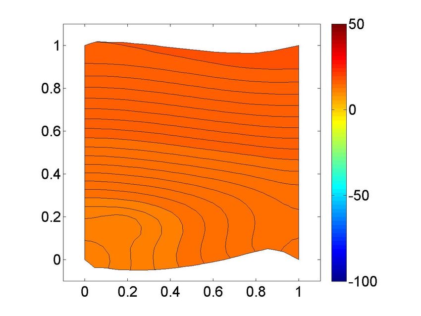
There exist one factor, called stretch, which is responsible for the activation and inactivation of the
mechanically controlled ion channels. In 1997, Hu & Sachs [HS97] revealed the stretch activated channels
(SACs) in cardiac cells. Positive response of the SACs contribute for heart to stretch. Cardiac muscle stretch
also leads to the increase in active tension.
    For the finite elasticity material, there are various models for the strain energy function based on the
different laws. For example, in [GCM95a] Guccione et al. used the transversely isotropic exponential law
strain energy function and the orthotropic and isotropic laws have been used in [NP04] and [CBP+ 14a],
respectively. Various models for the development of the active tension and the description of the dynam-
ics of calcium ions and the cross bridges bindings have been proposed in [CBP+ 14b, DGKK13, EPPH13,
KNP09, KOMM10, MW07, RLRB+ 14, SMCCS06, WGRS11, PW09, LNA+ 12a, JGT10, GLC+ 11, GCRT10,
DORB+ 13, CHLT13, AHZ13a]. In [HMTK98], Hunter et al. presented the model based on the review of
experimental data for the mechanics of active and passive cardiac muscle. They concluded that it could be
interpreted as the four state variable model. (i) myocardial tissue passive elasticity, (ii) tension dependence
on the troponin C and Ca+2 bindings, (iii) tropomyosin movement kinetics and the actively cycling cross-
bridges binding sites and the length dependence of this process, and, (iv) cross-bridge tension development
kinetics under variations of the myofilament length. In [NS07], developed a biophysically and dynamically
stable model for the cardiac myocyte of rat at the room temperature. This model is capable of determining
the changes in the concentration of intracellular calcium ion in response to the stretch. In [LNA+ 12b],
presented a multiscale electro-mechanical model for the murince heart which is capable of investigating the
effects of excitation-contraction coupling. In this paper,they show a strong relation between the tension and
the velocity to explain the differences between the single cell tension and the whole organ pressure transient.
    For the cardiac electrical activity models at the tissue level, Bidomain and Monodomain models have
been considered in various researches [CHLT13, DORB+ 13, GCRT10, JGT10, WGRS11, DGKK13, MW07,
RLRB+ 14, EPPH13, KNP09, KOMM10]. For the ionic membrane models related to the different species
has been used in [CHLT13, DORB+ 13, GCRT10, JGT10, WGRS11, DGKK13, KNP09, KOMM10, MW07,
RLRB+ 14, EPPH13] etc.
    Following the electro-mechanical coupling approach presented in [AHZ13a, DORB+ 13, GCRT10, WBG07,
RLRB+ 14, PCGW10, NQRB12, PW09, NSH05, KNP09, GK10a, DGKK13, AANQ11] we need to impose
the electrical models on the deformed domain to propose the coupling between the electrical and mechanical
model. Then by the Lagrangian framework again this model is reformulated into the reference domain.
    There exist coupled cardiac electro-mechanical models which explain the traveling of electric signal into
the cardiac muscle and the contraction-relaxation process. These models consists : 1) the electrical model at
the tissue, which consists, the system of non-linear parabolic reaction-diffusion equations of the degenerate
type, 2) the cell level model to describe the flow of ionic currents via cellular membrane consist, system of
ordinary differential equations (ODEs), 3) deformation of cardiac tissue is modeled by the quasi-static finite
elasticity model, 4)intracellular calcium dynamics and the cross bridges bindings are described by the active
tension model which consists of a system of non-linear ODEs. Existence and uniqueness for the coupled
electro-mechanical model is given in [ABQRB15, BMST18].
    Cardiac arrhythmia involves the abnormality in the pattern of the heartbeat, if the electrical impulse
fails to start from the SA node or if there is some abnormality in the impulse initiated from the SA node.
Myocardial ischemia takes place when there is abnormality in the blood flow to heart and in oxygen supply
to the heart. It is one of the main causes of sudden death. Cardiac arrhythmia and heart attack can also
occur due to the myocardial ischemia. Due to this myocardial ischemia metabolism, electrophysiological
and mechanical changes appear which results in the reduction of action potential duration (APD), action-
potential upstroke, resting-potential shift, reduction in conduction velocity (CV), active tension, stretch
along the fiber and the stretch rate in the ischemic cells or tissue [2, 3, 4].
    Various experimental and numerical simulation work have been carried out to analyze the electrophys-
iological and metabolic properties of the healthy and ischemic cells and tissue [DMZ+ 16, JW89, PC87,
TRET07, CFPS07, RHR+ 08]. Mathematical and computational studies have been focused on investigating
various physiological effects in order to understand the relationship between the electrophysiological and
metabolic parameters. It can be analyzed from the past studies that these variations are basically due to, a)
Hyperkalemia which affects the cardiac cell resting potential due to the increase in the concentration of extra-
cellular potassium [SSCF90, PWM+ 10], b) Hypoxia defined as the reduced oxygen supply, it reduces the cell
metabolism and ADP to ATP concentration ratio in the cell get changed. Successively, this change affects

                                                       2
the opening of the particular ATP-dependent potassium channels [WL94, WVL92]. This ATP-dependent
potassium channels is also modulated by the mechanical environment.
    There are several research papers in which they have studied about ischemia in the animals. [FBS+ 85,
Car99, FKF+ 91, Cor94, MW07, PKZ+ 11, WTJC+ 86, SSCF90]. Since it is difficult to get the human data,
and hence it is challenging to extend the properties from animals to human. But it can be achieved via
computational modeling. Even though many human models have been built and analyzed via healthy cell
data their appropriateness for the ischemia computation is not known. So, it is essential to examine the
effect of varying ischemic parameters in the ischemic region. In [AP96, STO+ 00, TSO+ 00], studies have
been done for the global ischemia in human under different ischemic conditions. In [PKP19], the authors
has discussed the effect of local cardiac ischemia on the electrical activity of the ischemic region and the
neighboring healthy region in a human cardiac tissue.
    For the electro-mechanical coupling models, the bio-electrical activity experiences three main feedback
from the mechanical deformation:
    1. conductivity feedback: the influence of the deformation gradient on the conductivity coefficients of the
       electric current flow model;
    2. convection feedback: the influence of deformation gradient and deformation rate on the electric current
       flow model;
    3. ionic feedback: the influence of stretch-activated membrane channels on the ionic current.
    In [CFPS16] authors considered these three cases together and study their effects in a strongly coupled
anisotropic cardiac electro-mechanical model. X. Jie et al. [JGT10] used a electromechanical model for the
ventricle of rabbit to analyze the arrhythmia originates from the ischemia induced electrophysiological and
the mechanical changes. As per our literature survey no one has considered the electro-mechanical model of
the human cardiac tissue to analyze the local ischemia effects on the electro-mechanical activity.
    In this study, we will discuss the influence of local ischemic region on electrical and mechanical activity
in the deforming human heart. For the electrical activity at cell level, we will use the ten Tusscher human
ventricular membrane model [TTNNP04]. We will consider the above three cases (i), (ii), (iii) and study
the effect in deformed Monodomain model. We will also show the effect of ischemia on this model. We will
discuss the two types of ischemia namely Hyperkalemia and Hypoxia. We will discuss the influence of these
two types of local ischemia, by changing the corresponding parameters in the 2D tissue level model, on the
electrical and mechanical activity in terms of the action potential (AP), activation time (AT), repolarization
time (RT), action potential duration (APD) and intracellular calcium ion concentration [Ca+2 ]i , active
tension, (TA ), stretch (λ), stretch rate ( dλ
                                            dt ). We will also see the effect of the spread of ischemic zone in
both the ischemic subregion and the healthy region on the electrical and mechanical properties.
    In the next section, we will describe the cardiac electro-mechanical model and also discuss about the
ischemic parameters. We will also present the modeling of local ischemic zone. In the next section, we will
present the fully discrete system using finite elements in space and backward Euler method in time. In
section 4, we will discuss the numerical results.

2     Electro-mechanical models of cardiac tissue
Cardiac electro-mechanical model is a combination of electrical and mechanical models. In this section, we
will describe the mechanical and electrical models of cardiac tissue.

2.1     Cardiac tissue mechanical model
Let Ω̂ is the undeformed cardiac domain and Ω(t) is the deformed cardiac domain at time 0 t0 with X =
(X1 , X2 ) and x = (x1 , x2 ) are the spatial coordinates respectively.
   Define the deformation map, ψt (X) = ψ(X, t) = x from Ω̂ to Ω(t) and u(X, t) = x−X as the displacement
vector.
   In this work, cardiac tissue is considered as a nonlinear elastic material.
                                                          ∂xi
The deformation gradient tensorF (X, t) = {Fi,j } = { ∂X    j
                                                              , i, j = 1, 2, 3},

                                                       3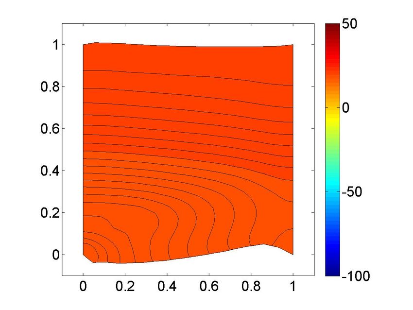
J(X, t) = detF (X, t)
Cauchy-Green deformation tensor C = F T F ,
Lagrange-Green strain tensor  = 21 (C − 1).
Also the deformed body satisfy the following steady state force equilibrium equation described as

                                          div(F S(u, X)) = 0, X ∈ Ω̂,                                        (1)

where S is the second Piola-Kirchoff stress tensor. Prescribed displacement is imposed on the Dirichlet
boundary x(X, t) = x̂(X), X ∈ ∂Ω   ˆ d and Neumann boundary with no traction force nt F S(u(X, t), X) =
0, X ∈ ∂Ωˆ n.
    The second Piola-Kirchoff stress tensor S, as taken in the studies [HMTK98, KBK+ 03, VM00, CFPS16],
is the combination of three components namely,

                                              S = SA + SP + SV ,

where active component S A generated biochemically, passive elastic component S P and volumetric compo-
nent S V .
   Next, S P,V is defined as follows

                                        1 ∂W P,V     ∂W P,V

                                   P,V
                                  Sij =           +           , i, j = 1, 2,                        (2)
                                        2   ∂ij      ∂ji

    where W P,V are the passive and volumetric strain energy functions, variety of these has been proposed
in [CHM01, GCM95b, HO09, GK10b, SNCH00, RNH05, SNYH06, UMM00] and  is the Green-Lagrange
strain.
    In this work, cardiac tissue is modeled as an orthotropic hyperelastic material. The passive strain energy
function for a hyperelastic material is given as in [EPPH13]:
                                              1
                                         W P = (eQ − 1),
                                             X2
                                         Q=     bi (I4i − 1)2 + blt I8lt
                                                                     2
                                                                         ,
                                              i=l,t

   where I4l = b̂Tl C b̂l , I4t = b̂Tt C b̂t and I8lt = b̂Tl C b̂t ,
   and volumetric strain energy function for a hyperelastic material is given as

                                               W V = K(J − 1)2 ,

where K is a positive bulk modulus.
   Now, the active component of second Piola-Kirchoff stress tensor S A is defined in the form of active
tension originated along the myocytes.
   An isometric contraction of the cardiac tissue, generates an active tension without changing length of
the cardiac tissue. Mechanical model of active tension is modeled by the myofilaments dynamics activated
by calcium. We consider, as suggested in [CFPS16], that the active force moves only in the fiber direction.
Therefore, active Cauchy stress is given as

                                        σ A (x, t) = J −1 TA al (x) ⊗ al (x),                                (3)
               F âl
   where al = |F âl | is a unit vector parallel to the local fiber direction and TA is the active tension in the
deformed domain.
   The active component of second Piola-Kirchoff stress tensor S A is defined as

                                              S A = JF −1 σ A F −T ,                                         (4)

and the stretch rate along the fiber is defined as
                                                       q
                                                  λ=    âTl Câl .                                          (5)

                                                         4
The active tension is dependent on calcium dynamics, stretch and stretch rate i.e. TA = TA (Cai , λ, dλ
                                                                                                        dt ),
as discussed in [LNA+ 12b] is given by the system of ODEs:

                                                              ntrpn
                     d(trpn)                         Cai
                               = ktrpn                                  ,
                         dt                 Ca50 (1 + β(λ − 1))

                     dXb                                                     1
                            = kXb (trpn50 )(trpn)nXb (1 − Xb) −                        Xb  ,
                       dt                                           (trpn50 )(trpn)nXb
                     dqi       dλ
                          = Ai     − αi qi , i = 1, 2,
                      dt        dt
                     TA = g(q)h(λ)Xb, q = q1 + q2 .                                                           (6)

where, function g(q) is the effect on tension is defined as :
                                                 ( aq+1
                                                       1−q         q≤0
                                          g(q) =      1+(a+2)Q
                                                         1+q       q>0
.
    For more details refer to [LNA+ 12b].

2.2      Cardiac tissue electrical model on a deforming domain: Monodomain model
We assume that the cardiac tissue is insulated. The influence of the cardiac tissue deformation on the
Monodomain model in the strong coupling framework is due to three different mechano-electrical feedback:
a) presence of deformation gradient F in the conductivity coefficients structure, b) presence of deformation
gradient F and the deformation rate in the conductive term, and c) presence of stretch λ in the Iion .
   Monodomain model on the deformed domain Ω(t) is defined as follows:

                     ∂v
                         − div(D(x)∇v) + Iion (v, w, c, λ) = Iapp , x ∈ Ω(t), 0 ≤ t ≤ T                       (7)
                     ∂t
                     ∂w
                         − g(v, w) = 0, x ∈ Ω(t), 0 ≤ t ≤ T                                                   (8)
                      ∂t
                     ∂c
                         − f (v, w, c) = 0, x ∈ Ω(t), 0 ≤ t ≤ T                                               (9)
                     ∂t
                     v(x, 0) = v0 (x, 0),    w(x, 0) = w0 (x, 0),  c(x, 0) = c0 (x, 0), x ∈ Ω                (10)
                       T
                     n D(x)∇v = 0, x ∈ ∂Ω, 0 ≤ t ≤ T                                                         (11)

where,

                                    D(x) = σl al (x)al T (x) + σt at (x)at T (x),

where, al (x) is a unit vector along the local fiber direction and at (x) is a unit vector transverse to the fiber
direction and they both are orthogonal to each other. σl and σt are the conductivity coefficients in the
corresponding directions.

                                      D(x) = σt I + (σl − σt )al (x)al T (x).

   Let v̂(X, t), ŵ(X, t), ĉ(X, t) and D̂(X, t) are the action potential, gating, concentration variables on the
undeformed domain Ω̂. Then

                                    ∂v̂   ∂v        ∂ψt
                                        =     + ∇v.     , (convective term)
                                    ∂t    ∂t         ∂t
                                    ∇v(x, t) = F −T Gradv̂(X, t),
                                    dx = JdX,

                                                         5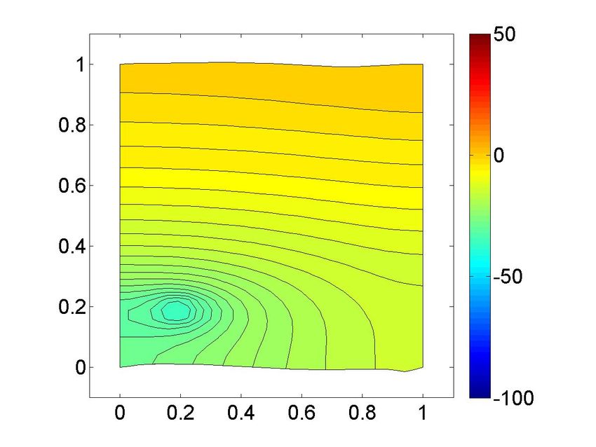
Thus the monodomain system on the reference domain Ω̂ is given as follows:

              ∂v̂    −T    dψt
          J       − F ∇v̂.       − div(JF −1 DF −T ∇v̂) + JIion (v̂, ŵ, ĉ, λ) = JIapp ,       X ∈ Ω̂,
              ∂t            dt

coupled with the system of ODEs for the gating and concentration variables w(x, t) and c(x, t) respectively,
given by
                           ∂w
                              − g(v, w) = 0,                                        X ∈ Ω̂, T               (12)
                           ∂t
                           ∂c
                              − f (v, w, c) = 0,                                      X ∈ Ω̂.               (13)
                           ∂t
Initial conditions:

                                v̂(X, 0) = v̂0 (X), X ∈ Ω̂,
                                w(X, 0) = w0 (X),         c(X, 0) = c0 (X), X ∈ Ω̂.                         (14)

Boundary condition:

                                nT F −1 D(x)F −T ∇v̂ = 0,          on      ∂ Ω̂ × (0, T ).                  (15)

Now, we compute the conductivity tensor D̂(X, t) on the reference domain is given as:

                               D̂(X, t) = F −1 D(x(X, t))F −T (X, t),              X ∈ Ω̂

We know the conductivity tensor in the deformed domain Ω(t) is defined as

                                      D(x) = σt I + (σl − σt )al (x)al T (x).

Now, let âl (X) is a unit vector parallel to the local fiber direction in the reference domain, then in the
deformed domain the unit vector al (x) along the local fiber direction is obtained by

                                                       F âl
                                                   al =        ,
                                                      kF âl k
                                                        F âl
                                                     =q
                                                        âTl Câl

Thus,

                                                          F âl âTl F T
                                               al aTl =
                                                           âTl Câl

2.3     Ionic model
Iion (v, w, c, λ), g(v, w) and f (v, w, c) are defined by the cell level model. In this work we are using the
human ventricular cell level model, ten Tusscher model [TTNNP04] (TT06). Dynamics of the ionic currents
is modeled by the 17 ODEs. The ionic current flow Isac due to the stretch activated channels and KAT P
current is also taken into account. Thus the total ionic current is given by

                       Iion = IN a + IK1 + Ito + IKr + IKs + ICaL + IN aCa + IN aK +
                            IpCa + IpK + IbCa + IbN a + IKAT P + Isac ,                                     (16)

   where, the fast sodium (IN a ), L-type calcium(ICaL ), transient outward(Ito ) , rapid delayed rectifier(IKr )
and slow delayed rectifier (IKs ), and inward rectifier currents (IK1 ), IN aCa is N a/Ca2+ exchange current,

                                                           6
D                                               C

                                   D1              C1
                                           (x,y)
                                                             (x',y')
                                    A1              B1

                            A                                                B

Figure 1: : Cardiac tissue ABCD with single ischemic subregion A1B1C1D1, (x, y) and (x0 , y 0 ) are
the points inside and outside the ischemic subregion.

IN aK is N a/K + pump current, IpCa and IpK are plateau Ca2+ and K + currents, IbCa and IbK are back-
ground Ca2+ and K + currents and IKAT P is theKAT P current, all are modeled as in [TTNNP04], IKAT P
which accounts for Hypoxia is defined as in [AP96]:
                                                                           0.3
                                                             [K + ]o

                                                                                         1
                         IKAT P = GKAT P fAT P                                                    (v − Ek ),   (17)
                                                              5.4                 40 + 3.5e0.025v

where, GKAT P is the conductance and Ek is the resting potential of potassium.
   Isac , the stretch activated current [AHZ13b] is given as follows :

                                             Isac = Isac,n + IKo ,
                                             Isac,n = Isac,N a + Isac,K ,

where, Isac,n is the non-specific current defined as follows:

                                                                       vR + 85
                                Isac,N a   = Gsac γslsac (v − vN a ) −          ,
                                                                       vR − 65
                                Isac,K = Gsac γslsac (v − vK ).

   The specific K + stretch-dependent current is given by
                                                           γsl,Ko
                                 IKo = GKo                               (v − vK ),
                                                   1 + exp(−(10 + v)/45)

where, γsl,Ko = 3(λ − 1) + 0.7.
    The two types of ischemia, Hyperkalemia and Hypoxia will be incorporated into the model by varying
the parameters corresponding to each of the two types of ischemia.
    Human Cardiac tissue is considered as a square ABCD, and the ischemic region is taken as a small
square A1 B1 C1 D1 . In this study, local ischemia is modeled by varying the ischemic parameter value in the
sub-domain A1 B1 C1 D1 only and using the normal value of the parameter in the remaining part of the cardiac
tissue ABCD. Also considering the ischemia as mild, moderate and severe by taking the [K + ]o parameter
value in the corresponding range in the domain A1 B1 C1 D1 only. Then, we compare the electrophysiological
properties of the ischemic and non-ischemic region points say (x, y) and (x0 , y 0 ) respectively (see Fig.(1)).

                                                                       7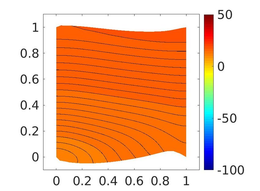
3      Weak Formulation
First of all we define the strong form the model. Monodomain model on the deformed domain Ω(t) is defined
as follows:

    (elasticity equation) − ∇.(∇uσ(x, γ)) = f,                                                        x ∈ Ω(t), a.e.t ∈ (0, T )
                                                                                                                             (18)
                            ∂v
    (Tissue level model)       − div(D(x)∇v) + Iion (v, w, c, λ) = Iapp ,                                x ∈ Ω(t), 0 ≤ t ≤ T
                            ∂t
                                                                                                                             (19)
                            ∂w
       (cell level model)      = G(v, w),                                                                x ∈ Ω(t), 0 ≤ t ≤ T
                            ∂t
                                                                                                                             (20)
                            ∂c
                               = h(v, w, c),                                                             x ∈ Ω(t), 0 ≤ t ≤ T
                            ∂t
                                                                                                                             (21)
                            ∂γ
                               = S(γ, w),                                                                x ∈ Ω(t), 0 ≤ t ≤ T
                            ∂t
                                                                                                                             (22)
                            v(x, 0) = v0 (x, 0), w(x, 0) = w0 (x, 0), c(x, 0) = c0 (x, 0),                           x ∈ Ω(t)
                                                                                                                           (23)
                            nT D(x)∇v = 0,                                                                x ∈ ∂Ω, 0 ≤ t ≤ T.
                                                                                                                          (24)

Now, we will define the general form of the ionic model so that the weak formulation of the above model
equations can be written.
   The general form of ionic current Iion : R × Rd × (0, ∞)n → R is defined as follows:
                                                       n
                                                       X
                                   Iion (v, w, c) :=         Qi (v, w, logci ) + R(v, w, c),                                 (25)
                                                       i=1

where,

                                         Qi ∈ C 1 (R × Rd × R),
                                                       ∂
                                         0 < H(w) ≤      Qi (v, w, ζ) ≤ H(w),
                                                      ∂ζ
                                           ∂
                                         | Qi (v, w, 0)| ≤ L(w),                                                             (26)
                                          ∂v
H, H, L ∈ C 0 (Rd , R+ ) and

                             R ∈ C 0 (R × Rd × (0, ∞)n ) ∩ Lip(R × [0, 1]d × (0, +∞)m ).                                     (27)

The following system of ODEs describing the dynamics of gating variables,
                                          ∂wi
                                              = Gi (v, wi ),          i = 1, 2, ..., d.                                      (28)
                                           ∂t
where, Gi has the particular form as

                               Gi (v, w) := αi (v)(1 − wi ) − βi (v)wi ,          i = 1, 2, ..., d,

and αi and βi are positive rational exponential functions in v.

                                                                8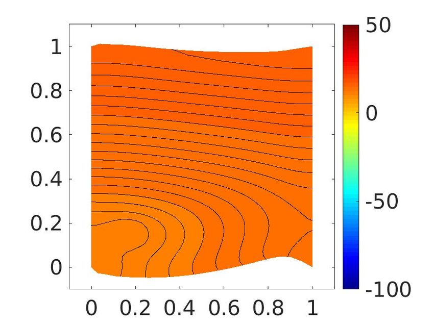
Assumption, ∀ i = 1, 2, ..., d,
                                Gi : R2 → R           is locally Lipschitz continuous,
                                Gi (v, 0) ≥ 0         ∀v ∈ R,
                                Gi (v, 1) ≤ 0         ∀v ∈ R.                                                          (29)
ODEs describing the dynamics of concentration variables is given by
                        ∂cj
                            = hj (v, w, cj ) := Qj (v, w, cj ) + Rj (v, w, cj ),        j = 1, 2, ..., n,              (30)
                        ∂t
where ,
              Rj ∈ C 0 (R × Rd × (0, ∞)n ) ∩ Lip(R × [0, 1]k × (0, +∞)m ), j = 1, 2, ..., n.      (31)
                                        Pk
The function S is given by S(γ, w) = β( j=1 ηj wj − η0 γ), where β and ηj are the positive pathological
parameters. Now, we will define the weak formulation of the above defined model.

3.1     Weak formulation
Definition: A weak solution of the problem (18)-(24) is a set (u, v, w, c, γ) such that u ∈ L2 (0, T ; H 1 (Ω)3 ),
v ∈ L2 (0, T ; H 1 (Ω)), vt ∈ L2 (0, T ; (H 1 (Ω))0 ), w ∈ C(0, T ; L2 (Ω)m ), c ∈ C(0, T ; L2 (Ω)n ), z ∈ C(0, T ; L2 (Ω)),
and it satisfy the following:
   ∀φ1 ∈ H 1 (Ω)3 , φ2 ∈ H 1 (Ω), φ3 ∈ L2 (Ω)m , φ4 ∈ L2 (Ω)n , φ5 ∈ L2 (Ω) a.e. t ∈ (0, T ) such that:
                          Z                          Z             Z
                             ∇uσ(x, γ) : ∇φ1 =           f φ1 dx +      uφ1 dx,                                         (32)
                          ZΩ           Z               Ω
                                                                  Z ∂Ω                   Z
                             ∂v
                                φ2 +        D(x, ∇u)∇v∇φ2 +           Iion (v, w, c)φ2 =    Iapp φ2 ,                   (33)
                             ∂t
                          ZΩ             ZΩ                         Ω                     Ω
                             ∂w
                                 φ4 =        G(v, w)φ3 ,                                                                (34)
                           Ω ∂t            Ω
                          Z            Z
                             ∂c
                                φ4 =        h(v, w, c)φ4 ,                                                              (35)
                             ∂t
                          ZΩ            ZΩ
                             ∂γ
                                φ5 =         S(γ, w)φ5 .                                                                (36)
                           Ω ∂t           Ω
                                 ∂u
Note: H 1 (Ω) = {u : u ∈ L2 (Ω), ∂x i
                                      ∈ L2 (Ω), i = 1, 2},
Note: L2 (Ω) = {u : Ω u2 < ∞}.
                    R

4     Numerical Scheme
The above electro-mechanical model is solved via finite element method for space discretization and implicit-
explicit (IE) Euler method for the time discretization.
    Cardiac tissue is discretized with rectangular grid The (grid size he ) for the electrical monodomain model
(12) and Thm (grid size hm ) for the mechanical model (1), where The is a refinement of Thm . We will then use
quadrilateral finite elements in space for both the electrical and mechanical models. For time discretization
of both electrical and mechanical models we will use equal time steps dt.
    We will solve this coupled electro-mechanical model in two steps:
    1) Time discretization of the ODEs to find w, c then solve the mechanical model to find the deformed
system.
    2) Solve the electrical monodomain model to compute v.
    1) a) Compute wn+1 , cn+1 , for a given v n , wn , cn , by solving (8) and (9) via Implicit- explicit Euler
method:
                                            wn+1 = wn + dtG(v n , wn+1 ),                                              (37)
                                                n+1      n          n    n+1     n
                                            c         = c + dtf (v , w         , c );                                  (38)

                                                                9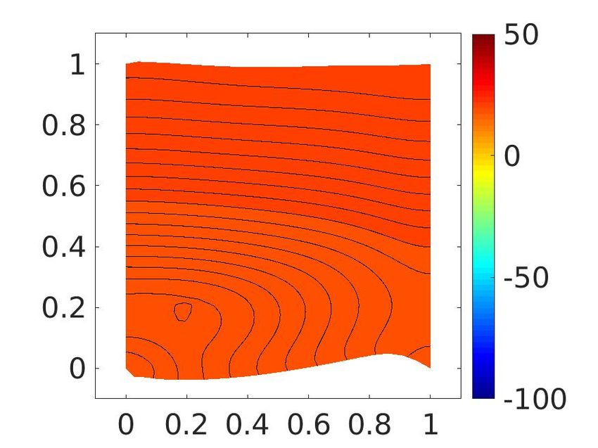
b) Now, use the obtained wn+1 , cn+1 to solve the mechanical model (1)- (6) and compute the new
deformed coordinates xn+1 in terms of the deformation gradient tensor F n+1 .
   2)Solve the electrical monodomain model using the linear finite elements in space and the IE Euler
method in time, for a given wn+1 , cn+1 and F n+1 and compute the action potential v n+1 .
   Define

                            Vh = {v ∈ H 1 (Ω) : vis continuous inΩ : v|E ∈ Q1 (E), ∀E ∈ The },
                            Wh = {u ∈ H 1 (Ω)3 : uis continuous inΩ : u|E ∈ Q1 (E), ∀E ∈ Thm }.

   After solving the ODEs, solve the mechanical equation using the FEM (mechanical discretization, Thm )
and calculate the deformation gradient at the next level.
   Choose {ξi }N             N
                i=1 and {ψi }i=1 as the basis functions in the space Vh and Wh respectively. Then we can
write the following:

                                                                              n
                                                                              X
                                                                      un =          au,i ψ n ,
                                                                              i=0
                                                                              Xn
                                                                      vn =          av,i ξn ,
                                                                              i=0

    The mechanical equation using the finite element method (mechanical discretization, Thm ) becomes as
follows:
                                                       Z               N
                                                                      X
                                                                 S∇           ui,t ψi (x) : ∇ψj = 0.
                                                           Thm          i=1

and then solve it using the Newton’s method.
   Also, solve the monodomain equation using the finite element method (electrical discretization, The ) in
space, the weak form of the monodomain equation becomes as follows:
                        Z         N
                                 X                       Z                             N
                                                                                        X                         Z
                                                                                                                                h
                                          vi,t ξi (x) ξj +              D(x, ∇u)∇                   vi ξi (x) ∇ξj =            Iion ξj ,
                        The         i=1                           The                      i=1                           The

          n
          X             Z                 n
                                          X            Z                                    Z                                        Z
                a0v,i           ξi ξn +         av,i       D(x, ∇ui,n )∇ξi ∇ξn +                    Iion (av,i , aw,i , ac,i )ξn =         Iapp ξn .
          i=0               Ω             i=0          Ω                                        Ω                                     Ω

This is an ODE in time which is now solved using the IE Euler method.

5    Results and Discussion
We will present the results computed from the numerical simulation performed via Matlab Ra2015 library.
Cardiac tissue is taken as a two dimensional slab of size [0, 1]2 . The conductivity tensor in two-dimension
we are using is as follows:

                                                   σ     0
                                             D= l
                                                    0 σt

We need to choose an appropriate grid system so that the numerical solution is computed up-to acceptable
accuracy. Such a goal is achieved through grid validation test. Prior to the grid validation we will briefly
discuss the discontinuity treatment of Iion expression due to ischemic subregions inside a healthy cardiac
tissue. While Hyperkalemic ischemic zones results in the discontinuity of [K + ]o parameter at the interface of
healthy and ischemic parts of a cardiac tissue the Hypoxic ischemic zones results in the discontinuity of fAT P

                                                                                10
parameter at the interface. Here these discontinuities are treated to a desired order of accuracy by a simple
regularization effect through appropriate interpolating polynomials. These local interpolating polynomials
of high order accuracy are constructed following the procedure discussed by Alsoudani and Bogle in [AB14]
using refined localized data around the discontinuity. Different grid systems consisting of (a) 441 (b) 625 (c)
841 (d) 1089 and (e) 2601 degrees of freedom (dofs) have been considered. We compare the action potential
obtained using these grid systems (as in [PKP19]). In all these cases only a marginal variation (less than
2–3% for 441 and 625 grids and 0.5% for others) is found.
The parameters value in the model is taken from the reference [CFPS16]. Applied stimulus Iapp is taken
as 200 mA/cm3 to start the depolarization process [CFPS16]. The initial condition for the action potential
and all the gating variables of the TT06 ionic model are taken as the corresponding resting values while the
boundary of the domain is assumed to be insulated.
Activation time (AT) is defined as the unique time τa (x) during the upstroke phase of the action potential
when v(x, τa (x)) = −50. Repolarization time (RT) is defined as the unique time τr (x) during the
repolarization phase of the action potential when v(x, τr (x)) = 0.9vR . Action potential duration (APD)
is defined as τr (x) − τa (x).
First of all, we will present the results for the simulation of the four situations S1, S2, S3 and S4 in the
cardiac tissue which are, (S1) without the mechanical feedback, (S2) consider the mechanical feedback into
the diffusion term of the Monodomain model but without Isac current and the convective term, (S3) Take
the mechanical feedback in the diffusion term and the Isac current, and, (S4) Take the mechanical feedback
in the diffusion term with Isac current and the convective term. We will also examine the impact on the
temporal variation of the action potential (v), intracellular calcium concentration ([Ca+2 ]i ), active tension
(TA ), stretch along the fiber (λ) and stretch rate ( dλ dt ) at the points (describe later) in the cardiac tissue
with the change of Hyperkalemia and Hypoxia both. We will also examine the increased ischemic region size
effect onto the non-ischemic region in terms of its electro-mechanical properties.
5.1 (Case 1) Cardiac tissue without ischemic subregion
5.1.1 Effect of S2, S3 and S4 situations on electrical and mechanical waveforms
We presented the action potential (v), intracellular calcium concentration ([Ca+2 ]i ), active tension (T ),
stretch along the fiber (λ) and stretch rate ( dλ
dt ) at the points (0.1875, 0.1875) (M1) and (0.5, 0.5) (M2) of
the human cardiac tissue (see Fig. (2), in the subsequent simulations M1 will be in the ischemic zone). The
simulations are plotted in Fig (2). From Fig. (2a) and (2b), it can be examined that action potential(v) for
the situations S1 and S2 i.e. without mechanical feedback and the addition of mechanical feedback without
Isac respectively, had a little difference. This implies that the addition of mechanical feedback had a little
effect on the cardiac electrical activity in terms of ventricular action potential profile and hence on QRS
complex of ECG.
Further, as we add the current generated due to the stretch activated channels i.e. Isac , the plateau phase,
repolarization phase and hence APD of action potential gets affected. Fast upstroke, early repolarization
and hence 10% decrease in APD is noticed. Next, with the addition of convective term i.e. S4, negligible
difference in action potential profile in comparison to S2 is noticed.
Since, S1 is without mechanical case, therefore, we will consider the mechanical parameters for the
situations S2, S3 and S4. Now, from Fig. (2c)- (2j), an alteration in the waveforms of the mechanical
parameters is noticed with the addition of Isac at the points M1 and M2 of the human cardiac tissue. With
the addition of the Isac , waveform of [Ca+2 ]i at the points M1 and M2 get affected during the resting phase
and hence the contractile force and the contractility. While addition of convective term does not affect the
contractility.
Stretch along the fiber (λ) and hence the stretch rate dλ dt changes with the addition of Isac . From Fig.
(2g) and (2h), it is to be analyzed that during the systolic contraction there is shortening of fiber i.e. λ < 1
and after this, myocyte stretch λ > 1. There is almost 1% change in the length of myocytes at point M1
and 3% change in the length of myocytes at point M2 relative to the resting length.
Thus, it is concluded that ventricular contraction without Isac had little effect on the action potential
and hence on ECG. With the addition of Isac i.e. stretch regulated electrical activities alter the AP phase as
repolarization phase and APD and hence alter the QRS complex and QT interval of ECG. The mechanical
stretch induced current Isac also changes the myocardial resting [Ca+2 ]i which is related to the changes in
11contractile force and hence contractility. This is consistent with the experimental studies (). Fiber length
also changes due to the stretch activated channels, which is responsible for the contraction and expansion
of the heart. In short, it is to be verified that the stretch activated channels plays an important role in the
electro-mechanical activity of HCT or in the functioning of the heart.
5.2 (Case 2) Cardiac tissue with ischemic subregion
We consider the cardiac tissue of size [0, 1]2 with ischemic subregion as [0.1563, 0.25]2 . The ischemic param-
eters [K + ]o and fAT P are varied in the subregion only. The impact of the change for these parameter values
are analyzed on the ischemic region and on the healthy neighborhood of the ischemic region. In this case, we
will examine the effect at points M 1(0.1875, 0.1875) and M 2(0.5, 0.5). M 1 lies inside the ischemic zone of
the cardiac tissue while M 2 lies in the healthy neighborhood of this ischemic region (see Fig. (3)). Now, we
will examine the electrophysiological and the mechanical properties of the cardiac tissue via action potential
(v), intracellular calcium concentration [Ca+2 ]i , active tension TA , stretch along fiber (λ) and stretch rate
( dλ
dt ) at these two points.
5.2.1 (a) Hyperkalemia (Effect of ischemia when only [K + ]o varies)
[K + ]o is taken in the range 5.4 − 20mM [SR97]. [K + ]o = 5.4mM is considered as the normal value. In Fig.
(4) and (5), action potential (v), intracellular calcium concentration ([Ca+2 ]i ), active tension (T ), stretch
along the fiber (λ) and stretch rate ( dλ dt ), at the points M 1 and M 2 corresponding to S2, S3 and S4 for
different values of [K + ]o is drawn. In Fig. (4), effect of Hyperkalemia at the point M 1 in the ischemic region
corresponding to S2, S3 and S4 can be easily visualized. With the increase in the strength of Hyperkalemia,
resting potential (RP) increasingly reaches to the higher level of potential values than that of the normal RP
value. RP corresponding to S2, S3 and S4 for [K + ]o = 20mM turns out to be -50mV while the RP for the
normal value of [K + ]o is -85mV. Thus, there is approximately 40% variation in the RP when Hyperkalemia
strength increases up to 20mM. For S2, the ischemic cell repolarize faster than that of the normal cell and
hence the APD also reduces with the increase in the Hyperkalemia strength also the cell gets activated earlier
as [K + ]o reaches to 20mM. This faster repolarization and reduction in APD at M1 is more evident with the
addition of the ionic current generated by the stretch activated channels i.e. (Isac ). While the addition of con-
vective term (i.e. S4) shows negligible change in AP. Changes in the values of APD at M 1 is given as follows:
S2 S3 S4
APD (at M1 when [K + ]o = 20mM) 272 265 264
From Fig. (5), we can see that at M2 there are small changes in all the phases of the action potential
for all the cases S2, S3, and, S4, when [K + ]o reaches to 20mM. Early depolarization, faster repolarization is
visible. With the addition of (Isac ) nearby healthy cell M2 goes faster to the resting state while the addition
of convective term shows negligible effect.
From Fig. (4d)- (4f)and (5d)-(5f), at M1 and M2, changes in the waveform of the concentration of the
intracellular calcium ions [Ca+2 ]i for the cases S2, S3, and S4 are negligible when [K + ]o ≤ 12mM . Changes
in the mechanical waveform of [Ca+2 ]i are visible when [K + ]o reaches 20mM and this change in [Ca+2 ]i
waveform leads to change in contraction force and hence contractility of the cardiac tissue. It is to be
noticed that at M 1 and M 2 the effect in the waveform of TA for the cases S2, S3, and S4 is negligible when
[K + ]o ≤ 12mM and the effect in the change in mechanical waveform of TA is visible when [K + ]o reaches to
20mM. It is also clearly visible that the influence of Hyperkalemia on the stretch along fiber λ and stretch
rate, dλ dλ
dt i.e. the change in the waveform of λ and hence dt is negligible at M1 corresponding to S2, S3 and
S4. The change in the waveform of λ and hence dλ dt is more at the point M2 i.e. stretch along the fiber and
stretch rate is more with the increase in Hyperkalemia strength. There is more than 3% change in the length
of the myocytes relative to the resting length at point M2.
AT, RT and APD contours for S2, S3 and S4 with [K + ]o = 20mM is presented in Fig. (6)- (8). From
Fig. (6), it is visualized form the isochrone lines that the addition of Isac does not affect the AT pattern.
Also, increasing the level of Hyperkalemia leads to a visible hastening in the activation of human cardiac
12(a) (b)
(c) (d)
(e) (f)
(g) (h)
(i) (j)
Figure 2: : v (a), [Ca+2 ]i (b), TA (c), λ (d), dλ
dt (e) for the cases, without MEF, without Isac , with
Isac and with Isac + CONV at M1(column1) and 13 M2(column2).Figure 3: : Cardiac tissue with one ischemic subregion, M 1 is the point inside the ischemic
subregion and M 2 is outside the ischemic subregion.
cells. An elliptic area is clearly visible which activated earlier than the surrounding one. This indicates that
ischemic region generate a new wave.
Fig. (7) and (8) indicates that due to the addition of Isac cardiac cells slightly repolarize faster and hence
reduces APD. Also the cardiac cells near to the ischemic region repolarize faster or RT of the ischemic cells
or neighboring to the ischemic cells reduces and hence these cells go to the resting state earlier and this
tendency increases as the Hyperkalemia gets severe.
In Fig. (9) and (10), we presented the action potential contours in deformation of the cardiac tissue with
the increase in the strength of Hyperkalemia, for S2 and S3, respectively. The change in the deformation of
cardiac domain with increasing the Hyperkalemic strength is clearly visible.
Next, the effect of increase in the size of the ischemic region from [0.1563, 0.25]2 to [0.0938, 0.3125]2
on action potential, intracellular calcium ions [Ca+2 ]i , active tension TA , stretch along the fiber λ and
stretch rate, dλ +
dt are presented in Fig. (11) for the case [K ]o = 20mM. Clearly the spread of severe
Hyperkalemic ischemic zone further raises already increased resting potential levels, at M 1, from -50mV to
-45mV respectively. Also the growth in ischemic size leads to faster repolarization with a reduced APD.
There is almost 9% further drop in APD is noticed with a factor of five times increase in the ischemic
subregion size. From the action potential plot corresponding to point M 2, it is visible that there is almost
5% drop in APD for this neighboring healthy cell. Thus, it is amply clear that in the proximity of ischemic
subregion the CEA in terms of action potential and hence the ECG of healthy cardiac tissue is affected with
the severity of Hyperkalemia. This effect in the ischemic and healthy cells will increase with the spread of
ischemic region.
It is also noticed that there is variation in the waveform of [Ca+2 ]i at M1 while it is going to rest, but at
M2 the waveform changes during all the phases. The variation in the stretch along the fiber and the stretch
rate is more in the neighboring region point M2 with the expansion of the ischemic region while the change
at the point M1 inside the ischemic region is negligible. In short, expanding the ischemic region size affect
the mechanical properties of the neighboring healthy cells more intensely.
Hence, it could be concluded that addition of Isac leads to ECG change and mechanical contraction as it
reduces the APD and affects the contractility and the length of length of myocytes of healthy and ischemic
parts of the human cardiac tissue. It is also observed that the severity of Hyperkalemia leads to reduction in
APD, elevation in resting potential, affects the contractile force and contractility and the stretch activated
channels, hence affects the QRS complex and QT interval of ECG and the mechanical contraction or can say
the electro-mechanical activity of healthy and ischemic regions of human cardiac tissue. All these effects on
14the electro-mechanical activity of a human heart gets more intense as the ischemic regions expands or more
cardiac cells becomes ischemic.
Note: As it is concluded that the addition of Isac plays an important role in the electro-mechanical
activity of a human cardiac tissue. So, next results will be with Isac case only.
5.2.2 (a) Hypoxia (Effect of ischemia when only fAT P varies)
fAT P is taken in the range 0.1 − 0.5%. Influence of the fAT P values (oxygen level) on the action potential
and the mechanical parameters [Ca+2 ]i , active tension (TA ), stretch along the fiber (λl ) and stretch rate
( dλ
dt ) at the two points M 1 and M 2 (described above) of the cardiac tissue are estimated and presented in
l
Fig. (12). From Fig. (12a), it can be seen that as the oxygen level in the ischemic region of the cardiac tissue
decreases (or fAT P value increased), delay in the closing of L-type Ca+2 channels is noticed, and further
rapid close of the K + channels takes place, therefore the plateau phase and then the repolarization phase of
the cardiac action potential get affected. Therefore, APD also reduces with the increase in the strength of
Hypoxia. While from the Fig. (12b), it can be seen that influence of the increase in fAT P values is negligible
on the neighborhood point M2 on the non-ischemic region of cardiac tissue.
Further from figures (12c) - (12j), it is visulaized that there is negligible change in the waveform of the
mechanical parameters, intracellular calcium concentration ([Ca+2 ]i ), active tension (TA ), stretch along the
fiber (λl ) and stretch rate ( dλ
dt ) at the points M 1 and M 2.
l
From Fig. (13a)-(13g), it is clear that the activation time remain unaffected by fAT P and hence the
isochrones of AT corresponding to these cases turn out to be same in the entire domain including those in
ischemic region. The front near the ischemic region is quasi elliptic and becomes flat after that.
RT isochrones show that as we increase the fAT P values in the ischemic region i.e. as the oxygen level in
the ischemic region of the cardiac tissue decreases, the cardiac cells in the ischemic region repolarize earlier
i.e. the repolarization time of ischemic cell decreases with the increase in fAT P values while the repolar-
ization time for the non-ischemic cardiac cells remains same. The loss of quasi-ellipticity and the folding
of repolarization time isochrones especially in the ischemic subregion depict an accelerated repolarization
wave propagation in the human cardiac tissue. The isochrone lines for APD shows that APD in the ischemic
region reduces as we are increasing fAT P values.
In Fig. (14a)-(14i), we presented the action potential contours in deforming cardiac tissue with the
increase in the strength of Hypoxia. We can visualize the change in the deformation of cardiac domain
with the increasing Hypoxic strength. Thus, change in oxygen level affects the contraction and expansion of
ventricle of human heart.
Next, as we increase the size of the ischemic region from [0.1563, 0.25]2 to [0.0938, 0.3125]2 , action potential
at the points M1 and M2 get influenced as shown in Fig (15). From the Fig (15a), we can conclude that, at
M1 (ischemic region point), with the increase in the size of the ischemic region there is further delay in the
closing of L-type calcium channels. Thus, a delay in plateau phase and then early repolarization of the action
potential takes place. APD also reduces with increase in the size of the ischemic region. From the action
potential plot corresponding to point M2 in Fig. (15b), a delay in plateau phase and early repolarization
of the action potential and reduction in the APD of these neighboring cells is also clearly visible. At M 1
there is 11% drop in APD with a factor of five times increase in the ischemic region size. Depending on the
distance of the neighboring points from the ischemic region, more than 5% drop in APD with a factor of five
times increase in the ischemic region size is noticed.
Now, from Fig. (15c) - (15j), it is visible that increasing the size of the ischemic region also considerably
affects the waveforms of the mechanical parameters [Ca+2 ]i , TA , λ and dλ dt corresponding to the point M1
than those of the point M2. From the figures (15g) and (15h), it can be noticed that an increase in the
size of the ischemic region by a factor of five leads to additional shortening of fiber length during systolic
contraction and an enhanced stretch in the fibers post systolic contraction. At M 1 3 − 4% change in the
length of the myocytes relative to the resting length is noticed and at M2 only a 1 − 2% change in the length
of the myocytes relative to the resting length is noticed. Therefore, the stretch rate dλ dt also changes at the
points M1 and M2 . There is approximately 45% variation in the stretch rate dλ dt at M 1 and approximately
5 − 25% variation in the neighboring points is detected.
Thus, the cardiac electro-mechanical activity mathematically generated by PDE-ODE system leads to
tracing of ionic channel dynamics, intracellular calcium ion abnormalities including the tissue structural
15(a) (b) (c)
(d) (e) (f)
(g) (h) (i)
(j) (k) (l)
(m) (n) (o)
Figure 4: : v (first row), [Ca+2 ]i (second row), TA (third row), λ (fourth row), dλ
dt (fifth row) for
the cases without Isac (first column), with Isac (second column) and with Isac + CONV (fourth
column) at M1, for different values of [K + ]o , data1 ([K + ]o = 5.4), data2 ([K + ]o = 12), data3
([K + ]o = 20)).
16(a) (b) (c)
(d) (e) (f)
(g) (h) (i)
(j) (k) (l)
(m) (n) (o)
Figure 5: : v (first row), [Ca+2 ]i (second row), TA (third row), λ (fourth row), dλ
dt (fifth row) for
the cases without Isac (first column), with Isac (second column) and with Isac + CONV (fourth
column) at M2, for different values of [K + ]o , data1 ([K + ]o = 5.4), data2 ([K + ]o = 12, data3
([K + ]o = 20).)
17(a) (b) (c)
(d) (e) (f)
Figure 6: : AT for the cases without Isac (first column), with Isac (second column) and with
Isac + CONV (third column) for [K + ]o = 5.4mM (first row) and [K + ]o = 20mM (second row).
(a) (b) (c)
(d) (e) (f)
Figure 7: : RT for the cases without Isac (first column), with Isac (second column) and with
Isac + CONV (third column) for [K + ]o = 5.4mM (first row) and [K + ]o = 20mM (second row).
18(a) (b) (c)
(d) (e) (f)
Figure 8: : APD for the cases without Isac (first column), with Isac (second column) and with
Isac + CONV (third column) for [K + ]o = 5.4mM (first row) and [K + ]o = 20mM (second row).
influences. It may be noted that the ionic channels corresponding to each cardiac cell adds to the generation
of cardiac action potential and also forms the basis for calcium induction, calcium release and cardiac
mechanical contraction. The change in the action potential phase and hence in ECG pattern affects both
the electrical and mechanical function of heart. These numerical results help in tracing the affected action
potential phase, leading to a disturbance in ECG pattern. It also helps in identification of corresponding
affected ionic channel dynamics. Thus, the current analysis can provide a useful guideline for the treatment
of Hyperkalemia and Hypoxia.
Thus, the heart failure due to the cardiac disease from the abnormal functioning of the coupled electrical
and mechanical activity can be traced through the virtual reconstruction of ionic channels and intracellular
calcium ion abnormalities with cardiac structural reconstruction through the proposed numerical modeling.
The ionic channels corresponding to each cardiac cell adds to the generation of cardiac action potential and
also forms the basis for calcium induction, calcium release and cardiac mechanical contraction. The change
in the action potential phase and hence in ECG pattern affects both the electrical and mechanical function
of heart.
6 Conclusion
Local ischemia in the deformed human cardiac tissue is modeled by varying the ischemic parameters value
in the ischemic subregion of the cardiac tissue domain. Two types of ischemic effects, namely, Hyperkalemia
and Hypoxia, are considered in this work. Monodomain model in a deforming domain is taken with the
TT06 human cell level model. The coupled electro-mechanical PDEs-ODEs non-linear system of equations
are solved numerically using linear finite elements in space and backward Euler finite difference scheme in
time. We examine the cardiac electrical and mechanical activity in terms of the action potential (v) and
intracellular calcium ion concentration [Ca+2 ]i , active tension, (TA ), stretch (λ), stretch rate ( dλ
dt ), in several
cases for local ischemia. We investigated the effect of varying strength of Hyperkalemia and Hypoxia in the
19(a) (b) (c)
(d) (e) (f)
(g) (h) (i)
Figure 9: : Action potential contours in a deforming domain for the cases without Isac for
different values of [K + ]o = 5.4 mM (first column), [K + ]o =12 mM (second column), [K + ]o = 20
mM (third column), at time t=90 (first row), t=150 (second row), t=240 (third row).
20(a) (b) (c)
(d) (e) (f)
(g) (h) (i)
Figure 10: : Action potential contours in a deforming domain for the cases with Isac for different
values of [K + ]o =5.4 (first column), [K + ]o =12 (second column), [K + ]o = 20 (third column), at
time t=90 (first row), t=150 (second row), t=240 (third row).
21(a) (b)
(c) (d)
(e) (f)
(g) (h)
(i) (j)
Figure 11: : v(first row), [Ca+2 ]i (second row), TA (third row), λ (fourth row) and dλ
dt (fifth row), at
M1(first column), M2 (second column), for the 22 case with Isac (second column) for [K + ]o = 20,
with two different sizes of ischemic regions, data1 ([0.1563, 0.25] ), data2 ([0.0938, 0.3125]2 ).
2(a) (b)
(c) (d)
(e) (f)
(g) (h)
(i) (j)
Figure 12: :v(first row), [Ca ]i (second row), TA (third row), λ (fourth row) and dλ
+2
dt (fifth row), at
M1(first column), M2 (second column), for different
23 values of f AT P . data1 (fAT P = 0), data2
(fAT P = 0.1%), data3 (fAT P = 0.3%), data4 (fAT P = 0.5%).(a) (b) (c)
(d) (e) (f)
(g) (h) (i)
Figure 13: :AT (first column), RT (second column), APD (third column) for different values
of fAT P = 0(first row), fAT P = 0.1%(second row), fAT P = 0.3%(third row), fAT P = 0.5%(fourth
row).
24(a) (b) (c)
(d) (e) (f)
(g) (h) (i)
Figure 14: :AP contours in a deforming domain for different values of fAP T =0 (first row),
fAP T = 0.3% (second row), fAP T = 0.5% (third row), at time t=90 (first column), t=150 (seconf
column), t=240 (third column).
25(a) (b)
(c) (d)
(e) (f)
(g) (h)
(i) (j)
Figure 15: :v(first row), [Ca+2 ]i (second row), TA (third row), λ (fourth row) and dλ
dt (fifth row), at
M1(first column), M2 (second column), for the26case with Isac (second column) for fAT P = 0.3%,
with two different sizes of ischemic regions, data1 ([0.1563, 0.25]2 ), data2 ([0.0938, 0.3125]2 ).ischemic subregion of cardiac tissue, on the electrical and mechanical activity of healthy and ischemic zones
in the cardiac muscle. We also investigated the impact of increasing the size of the ischemic region on the
electrical and mechanical parameters of neighboring cells.
(a) With the severity of Hyperkalemia the concentration of extracellular potassium ions increase leading
to, (i) Fall in availability of sodium channels and a decrease in inward sodium current, (ii) AP comes to a
resting state significantly prior to reaching the normal resting potential level, and, (iii) Increased potassium
conductance leading to shortening of RT in turn shortens QT interval is noticed.
These changes in cellular ionic dynamics not only further alters the AT, RP, RT and APD of affected cells
with the spread of Hyperkalemic region but also increasingly alters the AP of healthy cells in its vicinity.
Also, this spread of Hyperkalemic region alters the waveform of the mechanical parameters [Ca+2 ]i , TA , λ
, dλ
dt of the ischemic and the neighboring healthy cells.
Thus, the severity of Hyperkalemia leads to reduction in APD, elevation in resting potential, affects the
contractile force and contractility and the stretch activated channels, hence affects the QRS complex and
QT interval of ECG and the mechanical contraction or can say the electro-mechanical activity of healthy
and ischemic regions of human cardiac tissue. All these effects on the electro-mechanical activity of a human
heart gets more intense as the ischemic regions expands or more cardiac cells becomes ischemic.
(b) Severity of Hypoxic ischemia, with a reduction in intracellular ATP concentration, affect both influx of
calcium ions and efflux of potassium ions and alters the normal functioning of calcium channels and balanced
potassium channels. The increase in intracellular Ca+2 levels completely disturbs the Phase1, Phase2 and
Phase 3 of AP. As the Hypoxically affected region increases, the Plateau phase, repolarization phase and
the APD corresponding to the AP of healthy cells in its vicinity are affected and the ionic dynamics of
Hypoxically already degenerated cells get further disturbed. It is also visible that increasing the size of the
ischemic region by a factor of five considerably affects the waveforms of the mechanical parameters [Ca+2 ]i ,
TA , λ and dλ dλ
dt . There is approximately 45% variation in the stretch rate dt at M 1 and approximately 5−25%
variation in the neighboring points is detected.
Thus, the change in the action potential phase and hence in ECG pattern affects both the electrical and
mechanical function of heart. These numerical results help in tracing the affected action potential phase,
leading to a disturbance in ECG pattern. It also helps in identification of corresponding affected ionic channel
dynamics. Thus, the current analysis can provide a useful guideline for the treatment of Hyperkalemia and
Hypoxia.
Financial disclosure
We would like to thank the DST for support through Inspire Fellowship, ID no. is IF130906. We would also
like to thanks the ICTP-INdAM.
CONFLICTS OF INTEREST
The authors declare no potential conflict of interests.
References
[AANQ11] Davide Ambrosi, Gianni Arioli, Fabio Nobile, and Alfio Quarteroni. Electromechanical coupling
in cardiac dynamics: the active strain approach. SIAM Journal on Applied Mathematics,
71(2):605–621, 2011.
[AB14] Tareg M Alsoudani and Ian David Lockhart Bogle. From discretization to regularization of
composite discontinuous functions. Computers & Chemical Engineering, 62:139–160, 2014.
[ABQRB15] Boris Andreianov, Mostafa Bendahmane, Alfio Quarteroni, and Ricardo Ruiz-Baier. Solvability
analysis and numerical approximation of linearized cardiac electromechanics. Mathematical
Models and Methods in Applied Sciences, 25(05):959–993, 2015.
27[AHZ13a] Ismail Adeniran, Jules C Hancox, and Henggui Zhang. Effect of cardiac ventricular mechanical
contraction on the characteristics of the ecg: a simulation study. Journal of Biomedical Science
and Engineering, 6(12):47, 2013.
[AHZ13b] Ismail Adeniran, Jules C Hancox, and Henggui Zhang. Effect of cardiac ventricular mechanical
contraction on the characteristics of the ecg: a simulation study. Journal of Biomedical Science
and Engineering, 6(12):47, 2013.
[AP96] Rubin R Aliev and Alexander V Panfilov. A simple two-variable model of cardiac excitation.
Chaos, Solitons & Fractals, 7(3):293–301, 1996.
[BMST18] Mostafa Bendahmane, Fatima Mroue, Mazen Saad, and Raafat Talhouk. Mathematical analysis
of cardiac electromechanics with physiological ionic model. 2018.
[Car99] Edward Carmeliet. Cardiac ionic currents and acute ischemia: from channels to arrhythmias.
Physiological reviews, 79(3):917–1017, 1999.
[CBP+ 14a] Valentina Carapella, Rafel Bordas, Pras Pathmanathan, Maelene Lohezic, Jurgen E Schneider,
Peter Kohl, Kevin Burrage, and Vicente Grau. Quantitative study of the effect of tissue mi-
crostructure on contraction in a computational model of rat left ventricle. PloS one, 9(4):e92792,
2014.
[CBP+ 14b] Valentina Carapella, Rafel Bordas, Pras Pathmanathan, Maelene Lohezic, Jurgen E Schneider,
Peter Kohl, Kevin Burrage, and Vicente Grau. Quantitative study of the effect of tissue mi-
crostructure on contraction in a computational model of rat left ventricle. PloS one, 9(4):e92792,
2014.
[CFPS07] Piero Colli Franzone, Luca F. Pavarino, and Simone Scacchi. Dynamical effects of myocardial
ischemia in anisotropic cardiac models in three dimensions. Math. Models Methods Appl. Sci.,
17(12):1965–2008, 2007.
[CFPS16] Piero Colli Franzone, Luca F Pavarino, and Simone Scacchi. Bioelectrical effects of mechanical
feedbacks in a strongly coupled cardiac electro-mechanical model. Mathematical Models and
Methods in Applied Sciences, 26(01):27–57, 2016.
[CHLT13] Jason Constantino, Yuxuan Hu, Albert C Lardo, and Natalia A Trayanova. Mechanistic insight
into prolonged electromechanical delay in dyssynchronous heart failure: a computational study.
American Journal of Physiology-Heart and Circulatory Physiology, 2013.
[CHM01] Kevin D Costa, Jeffrey W Holmes, and Andrew D McCulloch. Modelling cardiac mechanical
properties in three dimensions. Philosophical transactions of the Royal Society of London. Series
A: Mathematical, physical and engineering sciences, 359(1783):1233–1250, 2001.
[Cor94] Ruben Coronel. Heterogeneity in extracellular potassium concentration during early myocar-
dial ischaemia and reperfusion: implications for arrhythmogenesis. Cardiovascular research,
28(6):770–777, 1994.
[DGKK13] Hüsnü Dal, Serdar Göktepe, Michael Kaliske, and Ellen Kuhl. A fully implicit finite element
method for bidomain models of cardiac electromechanics. Computer methods in applied me-
chanics and engineering, 253:323–336, 2013.
[DMZ+ 16] Sara Dutta, Ana Mincholé, Ernesto Zacur, T Alexander Quinn, Peter Taggart, and Blanca
Rodriguez. Early afterdepolarizations promote transmural reentry in ischemic human ventricles
with reduced repolarization reserve. Progress in biophysics and molecular biology, 120(1-3):236–
248, 2016.
[DORB+ 13] BL De Oliveira, BM Rocha, LPS Barra, EM Toledo, J Sundnes, and R Weber dos Santos. Effects
of deformation on transmural dispersion of repolarization using in silico models of human left
ventricular wedge. International Journal for Numerical Methods in Biomedical Engineering,
29(12):1323–1337, 2013.
28You can also read