Providing a foundation for road transport energy demand analysis: A vehicle parc model for South Africa - (SciELO) SA
←
→
Page content transcription
If your browser does not render page correctly, please read the page content below
Volume 29 Number 2

Providing a foundation for road transport energy demand
analysis: A vehicle parc model for South Africa

Adrian Stone1*, Bruno Merven2, Tiisetso Maseela3, Resmun Moonsamy4
1. Sustainable Energy Africa, Green Building, 9B Bell Crescent Close, Westlake Business Park, Tokai 7945,
   South Africa
2. The Energy Research Centre, University of Cape Town, Rondebosch, 7700, South Africa
3. Mott Macdonald, Cape Town office, Foreshore, 8001, Cape Town, South Africa
4. South African National Energy Development Institute, Block C, Upper Grayston Office Park, 152 Ann
   Crescent, Strathavon , Sandton, 2146, South Africa.

Abstract                                                  ton.km published by the University of Stellen-
It is key for national economic planning to build the     bosch’s Department of Logistics (2014 only). A
tools to forecast energy demand from major sectors        demand for passenger.km was also calculated,
like transport in a credible way. As a starting point,    which agreed well with national transport surveys. A
this requires building a sufficiently detailed ‘bottom-   range of detailed indicators were produced for the
up’ picture of technologies and their activity levels     vehicle typologies and some interesting trends
in the recent past. A vehicle parc model was devel-       observed, including the steady dieselisation of the
oped for South Africa to feed transport demand and        light vehicle fleet over the study period and the stag-
data on the fleet into a national energy systems          nation of passenger car fuel economy, despite legis-
model, the South African TIMES model, which is a          lation in the European Union. The present study
least-cost optimisation model of the TIMES/               believes that this updated data-rich picture of the
MARKAL family. Detailed assumptions were devel-           road transport vehicle parc will support other stud-
oped for 24 vehicle typologies that included the vin-     ies and national policy and planning initiatives.
tage profile, annual mileage and its relationship with
age, fuel economy and its improvement over time,          Keywords: freight demand, fuel economy, mode
and occupancy and load factor. Combining these            share, greenhouse gas emissions, vehicle fleets,
assumptions, the model was successfully calibrated        modelling
over 2000–2014 with the national registration
database, national fuel sales statistics and, on the
freight side, with estimates of the demand for

                               Journal of Energy in Southern Africa 29(2): 29–42
                          DOI: http://dx.doi.org/10.17159/2413-3051/2018/v29i2a2774

            Published by the Energy Research Centre, University of Cape Town      ISSN: 2413-3051
                                      http://journals.assaf.org.za/jesa

                           Sponsored by the Department of Science and Technology

* Corresponding author: Tel: +21 702 3622;
  email: adrian@sustainable.org.za

                      29 Journal of Energy in Southern Africa • Vol 29 No 2 • May 2018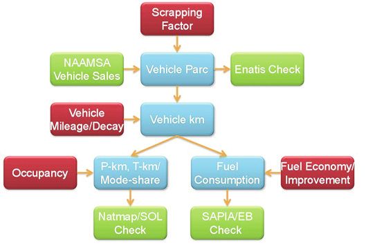
1. Introduction                                                   improving on some of the gaps identified in the pre-
The national energy balance for 2013 indicated that               vious work and presenting new work based on out-
the transport sector accounted for an estimated                   puts of a version of the SATIM energy systems
30% of South Africa’s total final consumption                     model that is linked to an economic model (Merven
(Department of Energy (DoE), 2013). The sector                    et al., 2017). This first paper will focus on the multi-
has remained almost completely dependent on liq-                  year calibration of the model using historical data
uid fuels, which accounted for 98% of demand in                   and present a detailed picture of the national freight
the sector in 2013 and 83% of all liquid fuels used               and passenger road transport system. The main
in the economy (DoE, 2013).                                       improvement on the previous work is a longer his-
    Large investments and long lead times are                     torical window for calibration and more granular
involved in meeting the demand for liquid fuels and               detail on heavy commercial vehicles so that the
transporting liquid fuels from point of supply to the             demand for freight (ton.km) could be calibrated to
point of demand. In addition, the choice of primary               the national figure published by the Department of
energy and the transformation process can have                    Logistics, University of Stellenbosch (Havenga, et
substantial impacts on society and the environment.               al., 2016a). The data-rich picture presented is
Investment decisions must, therefore, be informed                 intended to support the development of projections
by planning processes such as a national integrated               of transport energy sector demand for infrastructure
energy plan. The first step in the planning process is            planning purposes, the compilation of greenhouse
to build an understanding of the current demand                   gas inventories, and the assessment of greenhouse
for mobility of passengers and freight in the econo-              gas mitigation measures, amongst other uses.
my and the drivers of mobility in the transport sec-
tor and develop credible scenarios of how these will              2. The demographics of the vehicle parc in
evolve over time. Furthermore, the need for mobil-                South Africa
ity is not something that can be directly measured                South Africa is made up of nine provinces of
or observed and, therefore, requires estimation                   marked difference in size, population density and
based on a number of observable variables such as                 levels of economic activity, as shown in Table 1.
how many people are driving private vehicles, the                 Economic activity and car ownership are highly
demand for the movement of goods in the current                   concentrated in small but densely populated
economic environment, and how many vehicles are                   Gauteng, for example, in contrast to the arid and
on the road network (Merven, et al., 2012).                       sparsely populated Northern Cape. Three provinces
    The Energy Research Centre at the University of               – Western Cape, Gauteng, and Kwazulu-Natal with
Cape Town and the South African National Energy                   the country’s biggest port, Durban – together
Development Institute used the South African                      account for 55% of the population, 69% of regis-
TIMES Model (SATIM) in 2012, which is a least-cost                tered vehicles and 64% of gross domestic product.
optimisation model of the TIMES/MARKAL family,                    Much of this activity is concentrated in the cities of
to assess the demand for energy from transport to                 Cape Town, Johannesburg, Pretoria and Durban.
2050 (Merven, et al., 2012). The outputs of that                  This geography drives a large demand for transport,
study were widely applied (Department of                          allowing the country to be described as having a
Environmental Affairs, 2014; DoE, 2012; DoE,                      ‘spatially challenged economy’ (CSIR, 2013).
2016; Gajjar & Mondol, 2015). A series of papers,                     The average total motorisation for South Africa,
of which this is the first, will update these outputs,            estimated for mid-2016 at 192 vehicles per thou-

                     Table 1: Demographics and motorisation of South Africa’s provinces.
Province                Population     Total self-propelled     Share of      Motorisation Contribution to    Land area
                       (mid 2016)1           vehicles          vehicles (%)   (vehicle/1000 national GDP      share (%)
                                          (mid 2016)2                           persons)     (2015)3 (%)
Eastern Cape           7 061 700             719 939               6.7            102              7.8           14.0
Free State             2 861 600             527 459               4.9            184              5.1           11.0
Gauteng                13 498 200           4 163 142             39.0            308             34.0            1.5
KwaZulu-Natal          11 079 700           1 477 700             14.0            133             16.0            7.7
Limpopo                5 803 900             604 318               5.6            104              7.2           10.0
Mpumalanga             4 328 300             733 541               6.8            169              7.5            6.0
Northern Cape          1 191 700             234 453               2.2            197              2.1           31.0
North West             3 790 600             528 044               4.9            139              6.5            8.7
Western Cape           6 293 200            1 721 222             16.0            274             14.0           11.0
Total                  55 908 900          10 709 818            100.0            192            100.0          100.0
1   = StatsSA (2016a), 2 = eNaTiS (2016), 3 = StatsSA (2016)

                           30 Journal of Energy in Southern Africa • Vol 29 No 2 • May 2018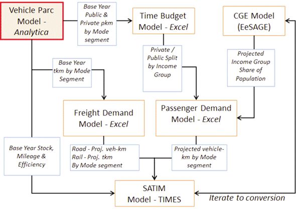
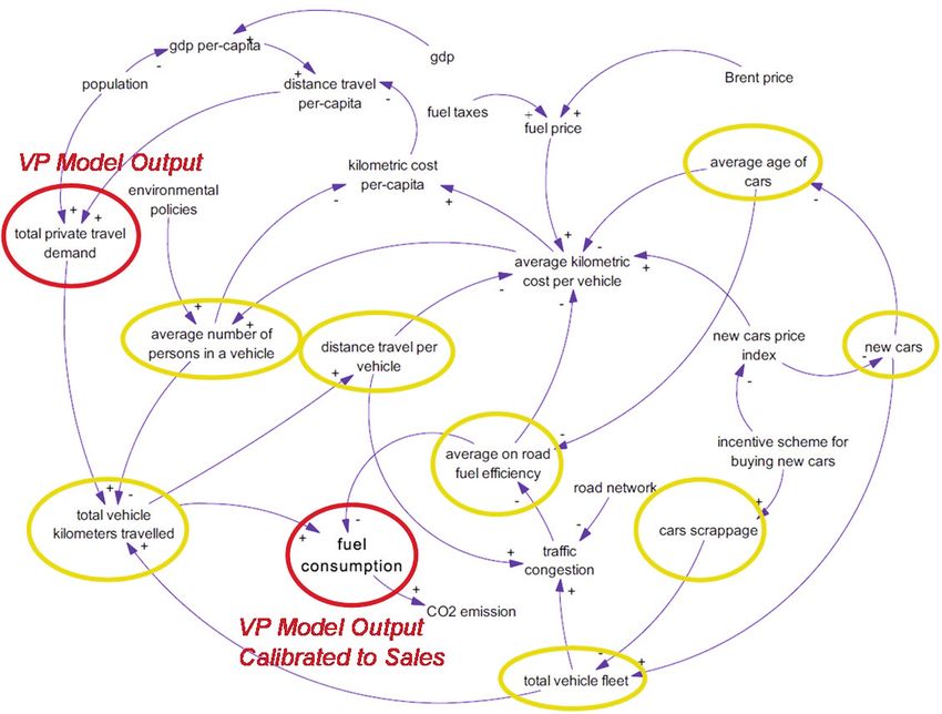
sand inhabitants, now just exceeds the global aver-       senger transport and illustrates the complex interac-
age of 180 and is considerably more than the              tions and extensive data needs required to effective-
African average of about 44 (Organisation Inter-          ly model this sector. A diagram for road freight
nationale des Constructeurs d’Automobiles, 2016).         transport would be similar, in that fuel consumption
But, even for the outlier of Gauteng, vehicle owner-      is still the direct result of vehicle-km travelled and
ship is significantly lower than the 500 to 800 for       vehicle fuel efficiency. Several of the elements in
developed countries and is more comparable to the         Figure 1 are included in the calibrated vehicle parc
BRICS counterparts of Russia and Brazil.                  model in the present study. These are: distance trav-
                                                          elled per vehicle, total kilometres travelled, fuel con-
3. Modelling transport demand                             sumption, fuel efficiency, total vehicle fleet, and
In a bottom-up approach, energy consumption by            average age of vehicles. Certain factors in Figure 1
any transport sector is directly driven by two factors:   affecting the vehicle-km travelled and fuel efficien-
vehicle-km travelled, and conversion efficiency of        cy, such as traffic congestion, are difficult to quantify
the vehicle (referring to a road, rail or air vehicle).   as they are not well understood locally. To compen-
The vehicle-km travelled are in turn driven by the        sate for this, the model was calibrated by adjusting
needs of society and the economy to move people           the variables until the output matches the known
and goods. Conversion efficiency depends mostly           fuel sales data. Once calibrated, the present study
on the underlying technology, i.e., type of vehicle,      could be reasonably sure that the model returns
fuel and vintage that make up the vehicle parc, and       realistic estimates of the number of operating vehi-
to some degree the patterns of utilisation of that        cles and their annual distance travelled. By making
technology. It is useful to treat passenger transport     an informed assumption regarding the average
and freight transport separately, as the needs for        occupancies of different vehicle types, total private
moving people and goods have slightly different           travel demand could be estimated.
drivers and technologies.
    (Armenia et al. 2010) proposed a detailed sys-        4. Research methodology
tems dynamics model, depicted by the causal loop          SATIM is an energy-economic-environment systems
in Figure 1, to represent the demand for mobility         modelling framework developed by the Energy
and energy consumption of passenger transport.            Research Centre, University of Cape Town (Altieri,
The model includes a number of drivers and inter-         2015; Energy Research Centre, 2015). It is devel-
actions which define energy consumption in pas-           oped according to ETSAP’s TIMES modelling

  Figure 1: Causal diagram for energy needs for passenger transportation (Armenia et al., 2010).

                      31 Journal of Energy in Southern Africa • Vol 29 No 2 • May 2018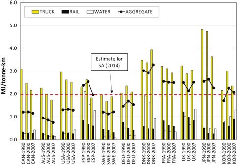
framework, which has been linked to a computa-            al., 2012) for this reason. This vehicle parc model
tional general equilibrium model known as eSAGE.          was updated for the present study and extended as
Both tools are developed using the general algebra-       follows:
ic modelling system, but a number of supporting           • heavy commercial vehicles which were a single
models developed on other platforms also support               aggregate in the first study were disaggregated
the modelling framework, as shown in Figure 2.                 into nine vehicle typologies to assist with cali-
    The present study focused on methodology,                  brating the model to the estimate of freight
assumptions and outputs of the vehicle parc model              demand (ton.km) published by the Department
component of the modelling framework hown in                   of Logistics, University of Stellenbosch (Hav-
the highlighted textbox in Figure 2. The function of           enga, et al., 2016a);
this model is to build a ‘bottom-up’ picture of the       • extension of the calibration window from seven
vehicle parc that can be used to generate a credible           to 14 years, spanning 2000–2013; and
estimate of the following key variables to enable the     • a parallel version in the open source R language
energy system model (TIMES) to project energy                  was coded to aid collaboration; final calibration
demand forward:                                                was performed in the R version.
• public and private passenger.km by mode/vehi-
     cle typology (e.g., gasoline minibus public or       4.1 Calculation and calibration
     diesel car private);                                 A schematic representation of the vehicle parc
• freight ton.km by mode/vehicle typology (e.g.           model and its data inputs and validations is shown
     gasoline light commercial vehicle (LCV)); and        in Figure 3. The procedure for calculation and cali-
• the stock, vintaged by age, of each typology            bration using the above parameters was broadly as
     and representative activity (annual mileage)         follows:
     and efficiency assumptions for each typology.        1. Historic vehicle sales data collected by the
     These assumptions need to be calibrated so                National Association of Automobile Manufac-
     that the fuel demand of the model matches sup-            turers of South Africa (Lightstone Auto, 2015)
     ply side data (fuel sales) as closely as possible.        were adjusted by scrapping curves to develop
                                                               an estimate of the stock of vehicles of different
     The road vehicle parc is characterised by a long          vehicle types for each model year, and the esti-
vintage window of around 30 years, given the high              mate was calibrated to the electronic national
average age of stock in South Africa. The character-           administration traffic information system
istics of new stock added and the activity levels of           (eNaTiS) registration database (eNaTiS, 2016)
old stock can change annually. Thus, while calcula-            by adjusting the rate of scrapping.
tions in this type of model are possible, the multipli-   2. Vehicle mileage estimates were developed for
cation of many large arrays is required. Lumina’s              both passenger and freight vehicles, assuming
Analytica platform (http://www.lumina.com/), an                that the annual mileage travelled by vehicles
array-based modelling tool with a powerful visual              decays from an initial value as they age.
interface, was selected for the first study (Merven et    3. Fuel demand was calculated by multiplying the

                           Figure 2: The SATIM transport modelling framework.

                      32 Journal of Energy in Southern Africa • Vol 29 No 2 • May 2018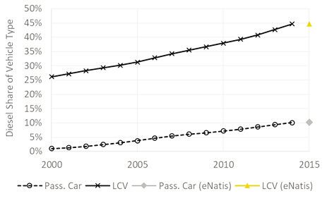
Figure 3: Schematic representation of the vehicle parc model and its data inputs and validations.

   kilometres travelled, the fuel economy, and the       used to estimate a diesel calibration target for the
   number of vehicles for a vehicle typology. The        model.
   typology fuel demands were summed to yield
   the vehicle parc fuel demand for gasoline and         4.3 Other calibration aspects
   diesel and compared with aggregate fuel sales         4.3.1 Vintage profile
   data.                                                 It is necessary to estimate the distribution of vehicles
4. An additional step for freight vehicles involved      of different ages and technology levels in the parc,
   adjusting the average maximum capacity,               known as the vintage profile, to assess the impacts
   capacity factor and mileage so that the model         of new technologies entering the market such as on
   calibrated not only against fuel sales but also       energy demand. The vintage profile can be deter-
   against published estimates of ton.km road            mined by establishing a distribution of the probabil-
   freight demand found in the literature (Hav-          ity of a vehicle surviving as a function of its age for
   enga, et al., 2016a).                                 each vehicle typology. Further detail on how this
                                                         was done is provided in the supplementary file.1
4.2 Vehicle typologies and calibration
targets                                                  4.3.2 Vehicle mileage
The typologies adopted for the vehicle parc model        The annual mileage of vehicles, when averaged
are presented in Tables 2 and 3, mapped to fuel          over a large number, appeared to decay steadily
type and more aggregate classifications. The aim for     from an initial value for each year of operation
the model was to calibrate model fuel demand             (Jackson, 2001; University of California at
against data on road transport fuel sales across a       Riverside, 2002). This is important because it
window of 2000–2014. In the case of gasoline,            means that older, more-polluting vehicles would
100% of sales were assumed to be used by road            contribute proportionally less to transport demand
transport, but this was challenging in the case of       than newer vehicles. This data is, however, not
diesel because, unlike gasoline, diesel is used for a    mandatory for capturing in the South African
wide range of off-road and stationary uses, includ-      licence-renewal process and was not available.
ing the fuelling of Eskom’s Ankerlig and Gourikwa        Mileage assumptions based on the United States
power stations since 2007. The South African             Environmental Protection Agency’s Mobile6 model
Petroleum Industry Association (SAPIA) and its           methodology (Jackson, 2001) were, therefore,
members disaggregate fuel sales using a quasi-sec-       adopted and scaled into the calibration process.
tor typology called trade categories, and this data is   Further detail on how this was done is provided in
then collated and made available on request by the       the supplementary file.
DoE (DoE, 2017). These categories offer some indi-
cation of what portion of diesel is used by road         4.3.3 Fuel economy
transport if an assumption of the share of road          The fuel economy of new vehicles was considered
transport diesel can be made for each trade catego-      to decrease by 0.5% per annum between 2000 and
ry. An assumed share of road transport in each           2014 for model implementation in the present
trade category was adjusted iteratively until there      study. This value was generally consistent with the
was a relatively smooth trend in the shares of the       more specific values in Europe during the period
sector demands over time, as shown in Figure 4.          used in the present study. Details can be seen in the
The resulting road transport share of diesel was         supplementary file.

                      33 Journal of Energy in Southern Africa • Vol 29 No 2 • May 2018
Table 2: Typology of vehicle parc model Table 3: Typology of vehicle parc model
mapped to aggregate categories: passenger mapped aggregate: Freight vehicles.
vehicles. Vehicle Weight Fuel type Model ID*
Vehicle type (eNatis Fuel type Vehicle parc type typology (kg)
and the SATIM model ID* LCVFigure 5: Calibrated vehicle parc model compared to the eNATiS registration database.
This allowed the split of the vehicle parc into its sprawl, so average trip distance is likely to be similar
typologies with some level of confidence, as pre- across modes, so motorised trip-based mode share
sented in Tables 4 and 5. and passenger.km mode share compare reasonably
The model indicated steady dieselisation of the well.
light vehicle fleet between 2000 and 2014, as Similarly, the demand for freight transport in
shown in Figure 6. The registration database ton.km was calculated by multiplying the calculated
(eNaTiS, 2016) has included a split between diesel vehicle.km with the assumed load factors, as pre-
and gasoline vehicles since 2015, and the model sented in Table 8, for each typology. In this case,
output compared well with this data. however, the load factors were derived from a cali-
The demand for passenger.km was calculated bration process against a published figure of 231
by multiplying the calculated vehicle.km with the billion ton.km for 2014 (Havenga, et al., 2016a).
assumed occupancy presented in Table 6 for each The detailed calibration results, including a split by
typology. The results show good agreement with vehicle typology and corridor, metropolitan and
other studies (NATMAP, 2005; NHTS, 2013). South rural operating environments are presented in
Africa’s car-driving, high-income households and Appendix A in the supplementary file.
low-income public transport users live in peripheral The energy intensity of road freight transport
Table 4: Vehicle typologies as a fraction of the Table 5: Vehicle typologies as a fraction of the
passenger road vehicle parc for 2010. freight road vehicle parc for 2010.
Vehicle typology Count of vehicles Fraction Vehicle typology Count of vehicles Fraction
(2010) (%) (2010) (%)
CarDiesel 221 779 3.6 LCVDiesel 852 698 33.2
CarGasoline 4 832 681 78.3 LCVGasoline 1 394 106 54.2
CarHybridDiesel 0 0.0 HCV1Gasoline 6 061 0.2
CarHybridGasoline 1 113 0.0 HCV1Diesel 120 270 4.7
CarElectic 0 0.0 HCV2Diesel 31 074 1.2
BusDiesel 21 686 0.4 HCV3Diesel 53 763 2.1
*MBTDiesel 23 911 0.4 HCV4Diesel 12 249 0.5
*MBTGasoline 277 064 4.5 HCV5Diesel 5 146 0.2
SUVDiesel 171 630 2.8 HCV6Diesel 74 175 2.9
SUVGasoline 252 050 4.1 HCV7Diesel 19 406 0.8
SUVHybridGasoline 541 0.0 HCV8Diesel 434 0,0
MotoGasoline 372 534 6.0 HCV9Diesel 514 0.0
Total 6 174 988* 100.0 Total 2 569 897* 100.0
* Total not calibrated to include the ‘Other self-propelled * Total not calibrated to include the ‘Other self-propelled
vehicles’ category in the eNaTiS registration database. vehicles’ category in the eNaTiS registration database.
35 Journal of Energy in Southern Africa • Vol 29 No 2 • May 2018Figure 6: Modelling trend in dieselisation of the light vehicle fleet compared with the registration
database for 2015.
Table 6: Model-generated passenger transport data for South Africa (2014).
Total Total Km per Occupancy Activity Modal share NATMAPa NHTSb
vehicles vehicle-km vehicle (person/ (billion (2014) (2005) (%) (2013)(%)
(1000 (billion (1000 vehicle, %) p.km) (%) of p.km of motor- of motor-
vehicles) vehicle-km) km) ised trips ised trips
Public
Large bus 23 0.61 26.1 25 15.2 6 10 8
MBT 278 7.40 26.6 14 103.7 38 40 35
Trainc 13.9 5 8 5
Sub-total 132.7 49 58 48
Private
Pass. car 5722 83.5 14.6 1.4 116.9 43.0 52.0
SUV 644 12.8 19.9 1.4 18.0 7.0
M/cycle 478 3.6 7.6 1.1 4.0 1.5 0.4
Sub-total 138.9 51.5 40.0 52.4
Grand total 271.6
(a) Source: DoT, 2009
(b) Source: Stats SA, 2013 – Calculated by mode taken on allocated travel day - NOT stated mode preference.
(c) Train data from literature, not the model - Intra city data only for 2006/2007 (Metrorail, 2007). Data for inter-city is not
published by the respective vendors
P.km = passenger, NATMAP = National transport masterplan, NHTS = National household travel survey, MBT = Minibus taxi.
was estimated to be 1.9–2.0 MJ/ton.km by dividing under 10%, except for the outliers in 2014 (11%).
the estimated diesel sales to road transport (the cal- The parameters input to the model in this study as
ibration target) and the model’s forecast of road compared with Merven et al. (2012) can be con-
freight diesel demand by the demand in ton.km. trasted using Phase 1 column in Table 7, and in the
The result compares favourably with international tables in the supplementary section. A comparison
data for similar markets, such as Australia (shown for gasoline cars only is presented in Table 7.
as AUS in Figure 7). Both fuel economy and mileage in the present
Figure 8 shows that the model had excellent study are about 10% lower, which may reflect an
agreement with both gasoline and diesel use during improved estimate because of the longer calibration
the calibration years 2000 to 2014, with the excep- window, but to some extent the differences also
tion of gasoline in 2014, thus providing validation arise from the pressure on the calibration of outliers
for the model and the indicators generated from it. in demand in 2008, 2013 and 2014. The possible
In the version of the model developed for the causes for this are discussed in more detail below.
present study, the calibration period was extended The data presented in Table 13 of the supplemen-
compared to the period used in Merven et al. tary file implies that the fuel consumption improve-
(2012), resulting in a relatively less-close fit to real ment was relatively low at 0.5% per annum over
world data, but still within acceptable bounds for the study period. The population of gasoline vehi-
this type of model. The standard deviation of errors cles, however, still grows at over 3% per annum,
was 4.8% for both gasoline and diesel and was well despite dieselisation. If vehicle mileage was con-
36 Journal of Energy in Southern Africa • Vol 29 No 2 • May 2018Figure 7: South African road freight (truck) energy intensity in 2014 compared to
selected OECD markets 1990–2007 (Eoma et al., 2012, Havenga at al., 2016a)
Figure 8. Model’s fuel demand vs actual fuel consumption for 2000 to 2014.
Table 7: Comparison of calibration parameters for gasoline cars between Merven et al. (2012)
and the present study.
Year Fuel economy (l/100 km) Annual mileage (km)
New Fleet average New Fleet average
Phase 1 2006 8.3 9.1 24 000 16 169
Present study 2014 7.8 8.2 21 000 14 457
stant, as assumed by the model, future growth in out empirical investigation. Most notably, local
gasoline demand would be sustained, as shown in authorities do not enforce its capture and the eNatis
Figure 8. It can, therefore, be deduced that the does not make the limited dataset that has been
recent drop in demand observed in the gasoline accumulated from partial completions available,
sales data is driven by consumers travelling less, despite the annual vehicle registration form histori-
while recognising the difficulty of verifying this with- cally having a placeholder for vehicle mileage. The
37 Journal of Energy in Southern Africa • Vol 29 No 2 • May 2018assumption of 0.5% fuel consumption improve- to the calibration from 2012 onwards, presumably
ment qualifies that the sources of error in the resulting from lower vehicle activity. Figure 8 shows
model’s fuel demand relative to observed sales is that gasoline demand recovered in 2015 and 2016
likely to include the following: in response to significant real price drops, while
• short- and long-run elasticity of demand in diesel demand remained low.
response to fuel price variations and average Travel time data suggests that congestion and
income due to consumers travelling less; trip distances have increased in South Africa (SEA,
• other effects on demand for private transport 2017), so another possible reason for the observed
like changing urban form and fluctuating con- drop in demand is data error. Historically, liquid
gestion; and fuels were supplied by a regulated oligopoly of the
• the error in the fuel sales data because of oil majors who collected detailed demand data to
changes in parties responsible for data collec- enable the complex distribution of fuels. The indus-
tion, compounded by changes in the structure try has changed as a result of competition legisla-
of the gasoline-fuels value chain. tion and legislation to enable access to the value
chain by historically disadvantaged entrants. This
The model is intended for passing parameters to resulted in the responsibility for data collection shift-
a long-term projection model. It does not attempt to ing from one of the majors – firstly to the industry
integrate price or income elasticities and assumes association, SAPIA, and then to the DoE. At the
that consumer preference for annual mileage is con- same time a number of independent wholesalers
stant over the period for a given vehicle age. emerged, including Afric Oil, Gulfstream Energy,
Considering that the vehicle population grew Mzumbe Oil, Women of Africa Fuel and Oils, Si-
monotonically over the study window, any signifi- yanda Petroleum, and Yem Yem Petroleum. These
cant drop in demand in response to price increase now deal in large volumes in some cases, building
would, therefore, result in significant error. The on a base of procurement by the state and state-
model responds indirectly to low economic growth owned enterprises (Transport World Africa, 2014;
through reduced car sales, but, as seen in Figure 5, Greve, 2013). This is to the extent that, while inde-
this effect is relatively dampened compared to the pendent wholesalers traditionally were not directly
fuel demand volatility seen in Figure 8. The periods surveyed for the national statistics, they are in some
of error in the calibration correspond to price cases believed to be importing fuel independently
volatility and economic growth variations as shown in large enough volumes to introduce significant
in Figure 9, with gasoline seemingly more respon- statistical uncertainty into the national energy bal-
sive to price fluctuations, and diesel more respon- ance(DoE, 2017b). The DoE has, therefore, not
sive to GDP/capita variations. only taken on a complex statistical function, but
The levelling off of GDP/capita caused by a performs this function at the time when the industry
struggling economy also seems to have depressed is rapidly becoming more complex and difficult to
demand for gasoline in a longer-run effect relative survey. It seems likely, then, that the levelling-off of
Figure 9. Gauteng gasoline and diesel prices and GDP/capita, 2000–2014.
38 Journal of Energy in Southern Africa • Vol 29 No 2 • May 2018gasoline demand is temporary and that economic be accounted for in the trend analysis. In addition,
recovery and ongoing improvement in data collec- the energy balances for those years (as published at
tion methods may see the official figure for gasoline the time of writing) suggest that the Eskom con-
demand rise again by the order of 2–3% per annum sumption was excluded from trade category data,
until there is a significant penetration of real-world, the total of which is equal to total final consumption
low-fuel economy vehicles into the vehicle parc. excluding transformation. Liaison with the DoE
A key aim of this study was to improve on pre- (2018), however, confirmed that the Eskom con-
vious work by calibrating freight demand from the sumption is indeed included in the trade category
model with that published by the Department of data and this was, therefore, adjusted downwards
Logistics, University of Stellenbosch. The number of by the additional amount before the share of road
freight vehicle typologies was increased and load transport was estimated. Improved statistical meth-
factors adjusted, taking some account of the limited ods will, however, only partly reduce uncertainty.
consultation (Havenga & Simpson, 2016b) that There is no substitute for empirical sector studies
was possible with the Department of Logistics with- and far more needs to be understood about energy
in the limitations of the present study. A data-rich use in the agriculture, construction and mining sec-
output was a calibrated split of ton.km by vehicle tors, if there should be any certainty that the resid-
typology and by region (corridor, rural and ual diesel in the calibration reflects that used by sta-
metropolitan), presented in Table 8. tionary and off-road activities.
The verified ton.km figure further enabled an The new freight data presented by the present
estimate of freight energy intensity for the country, study, however, represents a rare attempt to achieve
as presented in Figure 7. This calculation, however, agreement in key parameters across modelling
required an estimate of the diesel sales to road efforts by different teams in related fields, and will
transport as a calibration target and this can be con- hopefully be an example for improved collabora-
sidered uncertain given that it was derived from a tion, more effective validation, and better support
trend-smoothing exercise using sales data disaggre- for policy and planning in the energy and transport
gated by ‘trade category’, a legacy classification that spheres.
gives limited guidance on the commercial activity
the fuel was used for. The DoE is in the process of 6. Conclusions
moving to International Standard Classifications in A vehicle parc model for South Africa incorporating
its questionnaires (DoE, 2017b), which may enable detailed estimates for efficiencies and activity levels
more certain estimates in the future. A further for a variety of vehicle typologies was developed
uncertainty was that the diesel demand by Eskom and calibrated against national sales of gasoline and
was notably high during 2010–2015, and this must diesel over 15 years, from 2000–2014. The model
Table 8: Freight demand calibration output by vehicle typology and operating environment.
Assumptions (%) Model freight demand (billion ton.km)
SATIM Load factor Share of Share of Share of Total % share of Corridor Metro- Rural
vehicle type (ton/veh) ton.km ton.km ton.km demand politan
that is corridor that is metro that is rural
HCV1Diesel 1.4 0.4 86 14 7.77 3.4 0.03 6.67 1.07
HCV1Gasoline 1.5 8 75 17 0.06 0.0 0.00 0.04 0.01
HCV2Diesel 2.5 10 54 36 2.38 1.0 0.24 1.28 0.86
HCV3Diesel 5.0 24 62 14 16.19 7.0 3.81 10.11 2.27
HCV4Diesel 7.9 38 40 22 6.47 2.8 2.46 2.61 1.40
HCV5Diesel 10.9 53 31 16 3.96 1.7 2.11 1.22 0.63
HCV6Diesel 20.7 54 24 22 142.10 61.4 76.52 34.18 31.41
HCV7Diesel 18.6 55 16 29 31.51 13.6 17.29 4.97 9.26
HCV8Diesel 18.4 57 15 28 1.24 0.5 0.71 0.18 0.35
HCV9Diesel 21.9 57 17 26 0.70 0.3 0.40 0.12 0.18
LCVDiesel 0.4 0 84 16 8.89 3.8 0.03 7.46 1.40
LCVGasoline 0.4 0 82 18 9.98 4.3 0.02 8.19 1.78
tkm calibration comparison
Total 231.3 100.0 103.6 77.0 50.6
Dept of Logistics (Havenga, et al., 2016a) 231.0 103.4 77.0 50.6
Calibration error (%) -0.11 0.20 0.00 0.12
39 Journal of Energy in Southern Africa • Vol 29 No 2 • May 2018has 11 freight vehicle typologies that were used to accessibility of energy and environment data.
develop a parallel calibration of the ton.km demand Transport planning and planning for energy for
of the model with that estimated by the freight transport are particularly high on the national agen-
demand model of the Department of Logistics, da, with congestion in cities increasing, public trans-
University of Stellenbosch for 2014 (Havenga, et port networks expanding at great expense, and the
al., 2016a). This enabled an estimate of the energy costs of energy imports rising. The data-rich picture
intensity of freight transport for the country (1.9–2.0 provided by this model is, therefore, a useful input
MJ/ton.km) to be made, one that can be used to to many policy activities other than the projection of
benchmark the energy efficiency of the freight logis- energy demand. For example, extensions of this
tics industry. The model output furthermore pro- type of model are particularly useful for rapid
vides a data-rich picture of the activity levels, effi- assessment of the impacts on demand of disruptive
ciencies and contribution to meeting passenger and transport technologies, including battery electric
freight demand of different vehicle typologies. vehicles, hybrid electric vehicles and hydrogen fuel
Some interesting trends emerged from the time cell vehicles. This has relevance to the large gaso-
series of input and output data, as follows: line fuels sector in the country, which could be
• Steady dieselisation of the light vehicle fleet has severely affected by penetration of these technolo-
been occurring. gies. Future work will aim to explore these impacts.
• The fuel economy of the light vehicle fleet has
been improving only very slowly, if at all. Note
• The consumption of gasoline in particular has 1. Supplementary material can be found at https://jour-
dropped off steadily since 2011 and seems to nals.assaf.org.za/jesa/article/view/2774.
relate to lower activity levels, driven by eco-
nomic factors. References
Altieri, K. E., Trollip, H., Caetano, T., Hughes, A.,
The following important data issues emerged Merven, B., & Winkler, H. (2016). Achieving devel-
from the study: opment and mitigation objectives through a decar-
• In general, the quality of energy related data bonization development pathway in South
Africa. Climate Policy 16(sup1): S78-S91.
received was of concern in all the major
Armenia, S., Baldoni, F., Falsini, D. & Taibi, E., 2010. A
sources: fuel sales and registration statistics col-
system dynamics energy model for a sustainable
lated by government in partnership with indus- transportation system. Paper delivered at the ISDC
try, and vehicle sales data collated by industry Conference 2010, Seoul, South Korea.
and sold by a private concern as proprietary Bell, A., Stone, A. & Harmse, B., 2003. Final report
data. The following were key issues: investigation (desk top study) into the optimum
• Metadata is sparse or non-existent. future octane grade structure for South Africa –
• Obvious validation checks have sometimes Excel. Pretoria: Department of Energy (then
not been performed – for example, the sum Department of Minerals and Energy), Republic of
of disaggregates of the same commodity South Africa.
might not match or time series of quantities CSIR (Council for Scientific and Industrial Research).
have implausible step changes or trends. 2013. 10th Annual state of logistics survey for South
• A poor understanding of the technical details Africa 2013 – Bold steps forward. CSIR, Pretoria,
is sometimes apparent – for example, the dif- South Africa.
DEA (Department of Environmental Affairs). 2007.
ference between CO2 emissions and emis-
Long term mitigation scenarios. Pretoria: DEA (then
sions standards for local air pollutants.
Department of Environment and Tourism), Republic
• Older data has been removed from the pub- of South Africa.
lic record, so that developing time series is DEA (Department of Environmental Affairs). 2014.
difficult. South Africa’s greenhouse gas (GHG) mitigation
• The sparseness of activity data – for example, potential analysis. Pretoria: DEA (then Department
annual mileage over the life of the vehicle or of Environment and Tourism), Republic of South
vehicle occupancy and load factors necessitated Africa.
many assumptions. DoE (Department of Energy). 2013. National energy
• Diesel use in the agriculture, construction and balance for the Republic of South Africa, version 1.
mining sectors needs to be better understood in Pretoria: DoE.
order to make allocations of diesel use to sec- DoE (Department of Energy). 2012. Integrated energy
tors for modelling and greenhouse gas invento- plan 2012, Pretoria: DoE, republic of South Africa.
ry purposes with any certainty. DoE (Department of Energy). Integrated energy plan.
Part 1 of 3 ed. Pretoria: DoE, republic of South
Africa.
This study suggested that better energy policy
DoE (Department of Energy). 2017b. Personal commu-
and planning going forward requires stakeholders
nication.
to collaborate to improve the quantity, quality and
40 Journal of Energy in Southern Africa • Vol 29 No 2 • May 2018DoE (Department of Energy). 2017. Excel spreadsheet - values for passenger cars in Europe. The
fuel sales by trade category 1998–2015. Personal International Council on Clean Transportation.
communication. IEA (International Energy Agency). 2011. Sustainable
DoE (Department of Energy). 2018. Personal communi- mobility project (SMP) dodel – Excel spreadsheet
cation. forwarded by email. International Energy Agency.
DoT (Department of Transport). 2009. National trans- Jackson, M., 2011. Technologies to improve fuel effi-
port master plan (NATMAP) 2050 modelling report, ciency of heavy trucks. Presentation at workshop:
Pretoria: Department of Transport, Republic of European Commission, Reducing greenhouse gas
South Africa. emissions from heavy-duty vehicles: policy options,
EEA (European Environment Agency) 2016. Monitoring development and prospects – International work-
CO2 emissions from new passenger cars and vans in shop.
2015. European Environment Agency, Copenhagen, Jackson, T., 2001. Fleet characterization data for
Denmark. MOBILE6: Development and use of age distribu-
eNaTiS (Electronic National Administration Traffic tions, average annual mileage accumulation rates,
Information System). 2016. Live vehicle population and projected vehicle counts for use in MOBILE6.
as per the national traffic information system 2000- Assessment and Modeling Division Office of
2016. Available at: Transportation and Air Quality. U.S. Environmental
http://www.enatis.com/index.php/statistics/13-live- Protection Agency.
vehicle-population/537-vehicle-population-statistics- Lightstone Auto. 2015. Vehicle sales by type with associ-
for-june-to-july-2016. [Accessed January 2017]. ated technical data 1981–2014. Excel spreadsheet
Energy Research Centre, 2015. South Africa’s proposed collated and distributed on behalf of the National
nuclear build plan: An analysis of the potential Association of Automobile Manufacturers of South
socioeconomic risks. Technical report. Energy Africa.
Research Centre, University of Cape Town, Cape Merven, B., Arndt, C. and Winkler, H., 2017. The devel-
Town, South Africa. opment of a linked modelling framework for
Eoma, J., Schipper, L. & Thompson, L., 2012. We keep analysing the socioeconomic impacts of energy and
on truckin’: Trends in freight energy use and carbon climate policies in South Africa. WIDER Working
emissions in 11 IEA countries. Energy Policy 45: Paper 2017/40.
327–341. Merven, B., Stone, A., Hughes, A. & Cohen, B., 2012.
https://doi.org/10.1016/j.enpol.2012.02.040 Quantifying the energy needs of the transport sector
European Commission, 2017. Reducing CO2 emissions for South Africa: A bottom-up model. Energy
from heavy-duty vehicles. Available at: Research Centre, University of Cape Town, Cape
https://ec.europa.eu/clima/policies/transport/vehi- Town, South Africa.
cles/heavy_en#tab-0-0. Metrorail, 2007. National facts. Available at:
Gajjar, H. & Mondol, J., 2015. Technoeconomic com- http://www.metrorail.co.za/National_Facts1.html
parison of alternative vehicle technologies for South NAAMSA (National Association of Automobile
Africa’s road transport system. International Journal Manufacturers of South Africa ) / SAPIA (South
of Sustainable Transportation 10(7): 579–589. African Petroleum Industry Association) Working
https://doi.org/10.1080/15568318.2015.1026007 Group. 2009. Excel spreadsheet of the NAAMSA /
GFEI (Global Fuel Economy Initiative). 2016. Fuel econ- SAPIA working group vehicle car parc as used for
omy state of the world 2016 – Time for global the SAPIA gasoline and diesel study. Forwarded by
action. Global Fuel Economy Initiative. email August 2009.
Giannakidis, G., Labriet, M., Ó Gallachóir, B. & Tosato, OICA (International Organization of Motor Vehicle
G. (eds). 2015. Informing energy and climate poli- Manufacturers), 2016. Motorization rate 2014 –
cies using energy systems models: Insights from sce- worldwide. [Online].
nario analysis increasing the evidence base. RFA (Road Freight Association) 2009. Vehicle cost
Springer. schedule.
Greve, N., 2013. Transnet awards landmark R15.5bn Road Traffic Management Corporation, 2009. Road traf-
fuel contract to 9 black, women-owned firms. fic report – year 2008. Road traffic Management
Engineering News, December 2013.Available at: Corporation, an agency of the Department of
http://www.engineeringnews.co.za/article/transnet- Transport, Republic of South Africa..
awards-landmark-r155bn-fuel-contract-to-9-black- SEA (Sustainable Energy Africa). 2017. Sustainable
women-owned-firms-2013-12-05/rep_id:4136. energy solutions for South African local government
Havenga, J. & Simpson, Z. 2016b. Personal communi- – a practical guide. Cape Town: Sustainable Energy
cation on trends in freight logistics in South Africa. Africa.
Havenga, J., Simpson, Z. K. D., de Bod, A. & Braun, Stats SA (Statistics South Africa). 2013. Calculated from
M., 2016a. Logistics barometer South Africa 2016. the published survey data files for the National
Stellenbosch University, Stellenbosch, South Africa. Household Travel Survey 2013; available from
Heywood, J. 1988. Internal combustion engines funda- Datafirst, University of Cape Town. Datafirst,
mentals. Singapore: McGraw Hill. University of Cape Town.
ICCT (International Council on Clean Transportation). StatsSA (Statistics South Africa) 2016a. Statistical
2016. From laboratory to road: A 2016 update of release P0302, Mid-year population estimates 2016.
official and ‘real-world’ fuel consumption and CO2 Statistics South Africa.
41 Journal of Energy in Southern Africa • Vol 29 No 2 • May 2018Stats SA (Statistics South Africa). 2016b. GDP P0441
Annual, quarter and regional revisions tables - Q4
2016 Excel File. Statistics South Africa.
Stone, A.. 2004. Creating a national database of traffic
based vehicle emissions factors and vehicle parc –
Excel spreadsheet model supporting this publication.
Cape Town: National Association Of Clean Air
Western Cape symposium.
Stone, A. & Bennett, K., 2001. A bulk model of emis-
sions from South African diesel commercial vehicles.
Energy Research Centre, University of cape Town,
Cape Town, South Africa.
Transport and Environment, 2015. Europe’s lost decade
of truck fuel economy. Transport & Environment
Briefing.
Transport World Africa, 2014. Shaking up downstream
petroleum market. Available at: http://www.trans-
portworldafrica.co.za/2014/10/24/shaking-up-down-
stream-petroleum-market/.
University of California at Riverside, 2002. Kenya vehi-
cle activity study, Nairobi: Global Sustainable
Systems Research.
Vanderschuren, M., 2011. Personal communication –
Excel spreadsheet of vehicle model outputs.
Department of Civil Engineering, University of Cape
Town, Cape Town, South Africa.
42 Journal of Energy in Southern Africa • Vol 29 No 2 • May 2018You can also read


