Jamil, A.A., Hussain, F., Yousaf, M.H., Butt, A.M. y Velastin, S.A. (2020). Vehicle Make and Model Recognition using Bag of Expressions. Sensors ...
←
→
Page content transcription
If your browser does not render page correctly, please read the page content below
This document is published at:

Jamil, A.A., Hussain, F., Yousaf, M.H., Butt, A.M. y Velastin, S.A.
(2020). Vehicle Make and Model Recognition using Bag of
Expressions. Sensors, 20(4), 1033.

DOI: https://doi.org/10.3390/s20041033

   This work is licensed under a Creative Commons Attribution 4.0 International License.
sensors
Article
Vehicle Make and Model Recognition Using Bag
of Expressions
Adeel Ahmad Jamil 1 , Fawad Hussain 1 , Muhammad Haroon Yousaf 1,2 ,
Ammar Mohsin Butt 1 and Sergio A. Velastin 3,4,5, *
 1    Centre for Computer Vision Research, Department of Computer Engineering,
      University of Engineering and Technology, Taxila 47050, Pakistan;
      adeel.jamil@students.uettaxila.edu.pk (A.A.J.); fawad.hussain@uettaxila.edu.pk (F.H.);
      haroon.yousaf@uettaxila.edu.pk (M.H.Y.); ammarmohsin10@live.com (A.M.B.)
 2    Swarm Robotics Lab, National Centre for Robotics and Automation,
      University of Engineering and Technology, Taxila 47050, Pakistan
 3    School of Electronic Engineering and Computer Science, Queen Mary University of London,
      London E1 4NS, UK
 4    Zebra Technologies Corp., London SE1 9LQ, UK
 5    Department of Computer Science and Engineering, University Carlos III de Madrid,
      28270 Colmenarejo, Spain
 *    Correspondence: sergio.velastin@ieee.org

 Received: 22 December 2019; Accepted: 11 February 2020; Published: 14 February 2020

 Abstract: Vehicle make and model recognition (VMMR) is a key task for automated vehicular
 surveillance (AVS) and various intelligent transport system (ITS) applications. In this paper,
 we propose and study the suitability of the bag of expressions (BoE) approach for VMMR-based
 applications. The method includes neighborhood information in addition to visual words.
 BoE improves the existing power of a bag of words (BOW) approach, including occlusion
 handling, scale invariance and view independence. The proposed approach extracts features using a
 combination of different keypoint detectors and a Histogram of Oriented Gradients (HOG) descriptor.
 An optimized dictionary of expressions is formed using visual words acquired through k-means
 clustering. The histogram of expressions is created by computing the occurrences of each expression
 in the image. For classification, multiclass linear support vector machines (SVM) are trained over the
 BoE-based features representation. The approach has been evaluated by applying cross-validation
 tests on the publicly available National Taiwan Ocean University-Make and Model Recognition
 (NTOU-MMR) dataset, and experimental results show that it outperforms recent approaches for
 VMMR. With multiclass linear SVM classification, promising average accuracy and processing speed
 are obtained using a combination of keypoint detectors with HOG-based BoE description, making it
 applicable to real-time VMMR systems.

 Keywords: bag of expressions; intelligent transportation; make and model recognition; multiclass
 linear support vector machines; vehicular surveillance

1. Introduction
     Vehicle make and model recognition has emerged as a prominent problem in the computer
vision domain. There are many applications of VMMR in intelligent transport systems, including
vehicle monitoring, intelligent parking systems, searching suspicious vehicles, electronic toll collection,
autonomous vehicle systems, traffic analysis and so on. Another significant application of VMMR is
vehicular surveillance in sensitive security premises; e.g., parking lots of airports, universities, stadiums
and malls. An effective vehicle recognition approach is essential for acquiring high recognition

Sensors 2020, 20, 1033; doi:10.3390/s20041033                                  www.mdpi.com/journal/sensors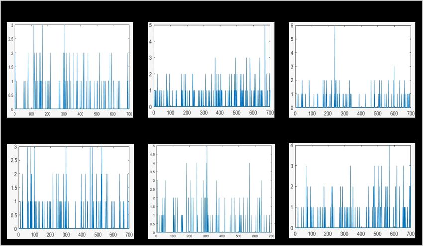
Sensors 2020, 20, 1033                                                                               2 of 19

accuracy. However, it is still a challenging task to recognize vehicle make and model in uncontrolled
environments due to occlusions, scale variance, specific classification problems and view dependencies.
In a traditional system, VMMR is based on a license plate recognition system or manual human
observations [1]. These two techniques have a low success rate and many limitations. For a human
observer, it is a laborious and time-consuming activity to remember and recognize a variety of vehicle
makes and models efficiently. License plate recognition systems have proven to be robust to various
lighting conditions with high processing speed and reasonable computational complexity [2]. On the
other hand, a VMMR based on a license plate recognition system can produce incorrect results due to
forgery, ambiguity, duplication or damaged license plates. Due to weaknesses in a traditional vehicle
recognition system, computer-vision-based automated vehicle make and model classification have
gained attention to improve an intelligent transportation system.
      Vehicle make and model (VMM) identification methods fall into three main categories in the
literature: feature-based, appearance-based and model-based methods. Feature-based methods identify
vehicle models based on global or local invariant features. Hence, their performance depends on the
reliability of features. For VMM, these have included symmetrical sped up robust features (SURF) [3],
edge map [4], sparse representation [5] and probabilistic feature grouping [6]. Hsieh et al. [3] proposed
a VMMR system using HOG and symmetrical SURF. Kumar et al. [7] detected vehicle logos by
combining appearance-based and feature-based methods, and then using an SVM classifier to classify
vehicles into four categories. Appearance-based methods classify vehicles by their inherent features
containing shapes [8], symmetry [9], textures and dimensions [10]. Variation in the pose or change
in the position of a camera can reduce the performances of those methods wherein the pose of
vehicles is estimated using shape features, as in [9], but the authors do not discuss occlusion,
lighting changes or viewpoint changes. Model-based recognition of vehicles includes the adaptive
model [11], the approximate model [12] and the 3D model [11,13]. In [11], to classify vehicles,
a 3D shape deformable vehicle model is used to detect different vehicle parts and then to recover
shape information.
      In this paper, we have opted for a feature-based method which is accurate and computationally
fast. In this class of methods, VMMR systems typically include the following modules: (a) vehicle
detection, (b) feature extraction and representation and (c) classification. Vehicle detection is a key step
for VMMR and has been investigated by many researchers. Faro et al. [14] implemented a background
subtraction procedure to subtract the vehicle region from the road, and then used a segmentation
technique to eliminate full and partial occlusions among blobs of the vehicle. In [15], Jazayeri et al. used
a hidden Markov model to probabilistically model the motion of the vehicle, and then to differentiate
vehicles from the road. However, such kinds of motion features are not applicable for single motionless
images. Because of color variation in vehicles, different color-based techniques have been used to
detect vehicles [4,16,17]. Chen et al. [18], proposed a symmetrical points projection approach for the
detection of vehicles from the background region.
      Recognition of inherent vehicle properties for VMM is useful for offline or online vehicle
identification, as compared to traditional license plate identification. To describe VMM on the basis
of the regions of interest, numerous local features are extracted, with or without representing local
features, into global features representations. The scale invariant feature transform (SIFT) [19] has been
applied in different VMMR works, such as [20–22], but the SIFT descriptor is computationally slow.
Baran et al. [20] used SIFT and SURF features and then embed them in a dictionary-based sparse vector
of occurrence sums. In [21] Fraz et al. extracted SIFT features to create a lexicon that includes features
of all the training images as words and then represents them by a fisher-encoded-based mid-level
representation. Manzoor et al. [22] used HOG and SIFT for feature extraction. In [1], local features were
extracted on the basis of Harris corners and gradient responses, and then locally normalized Harris
strengths (LNHS) or square-mapped gradients (SMG) were used for global feature representation.
He et al. [23], used edges and gradient-based features for feature extraction. For higher processing
speed, the SURF descriptor [24] has gained the attention of many researchers and has been used in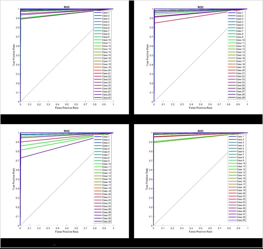
Sensors 2020, 20, 1033                                                                              3 of 19

different works, such as [3,25]. Heish et al. [3] proposed SURF to extract vehicle features in a grid-wise
manner and to represent them into grid-based global representation. In [25], Siddiqui et al. also
used SURF for feature extraction, and then adopted a BOW-based approach for global representation.
Two different techniques have been proposed for dictionary building in [25]: modular dictionary and
single dictionary. In [26,27] Nazir et al. proposed the dynamic spatio-temporal bag of expressions
(D-STBoE) model and the BoE framework for action recognition which improves the existing strength
of bag of words. A global feature ensemble representation is discussed by Chen et al. [18] who
combined the HOG vehicle features extracted in a grid-based pattern.
     In computer vision, numerous classification approaches have been used to improve the VMMR
classification process significantly. Psyllos et al. [28], apply a probabilistic neural network for
classification on the SIFT features extracted from vehicle images. A naive Bayes classifier is used for
the classification of VMM in [1]. For classification purposes, [23] reported the use of an ensemble of
neural networks as well as AdaBoost, SVM, and KNN. Varjas et al. [29] also proposed a KNN classifier
with an enhancement of a correlation-based distance metric. A euclidean distance-based matching
scheme is reported in [21], but it is a time-consuming task to match in a brute force manner. For the
classification of VMM, hamming distance and sparse representation approaches have been used in [18].
In [22], random forest classification is used for the recognition of VMM while Tang et al. [30] proposed
a nearest neighborhood classification approach for the recognition of vehicles. Jie Fang et al. [31]
and Afshin Dehghan et al. [32] describe a convolutional neural network (CNN) for the classification
of a vehicle’s make and model. Random forest and SVM are suggested for recognition of VMM
in [33]. Indeed, SVM-based classification schemes have been applied in different VMMR systems
such as [3,13,20,25]. In [34], the authors use a PCANet-based CNN for the recognition of a vehicle
make-model.

      Figure 1. Multiplicity problems with (a–c) Toyota Wish (C4) and (d–f) Honda CRV (C11) in the
      NTOU-MMR dataset. The multiplicity problem means one VMM often displays different shapes due
      to different manufacturing years.

     Some of the problems related to VMMR tasks are: varying image quality, variations in lighting
conditions, changes in weather conditions (rainy day, sunny day and night), viewpoint changes,
perspective distortion, etc. Shadows, backlighting conditions and occlusions can significantly change
visual properties. There are considerable variations in the size, color, orientation, pose and shape
between vehicles. Another major challenge in VMMR is multiclass classification. In this scenario,
there are two main categories: (a) multiplicity and (b) ambiguity. The former refers to the issue of
vehicle models of one make (company) having different shapes as illustrated in Figure 1; e.g., the “Wish”
models manufactured in 2010, 2009 and 2005 by “Toyota” have different visual appearances due
to shape upgrades. Similarly, the “CRV” models of the “Honda” make pose the same challenge.
The problem of ambiguity is further divided into two sub-problems: (a) intra-make ambiguity and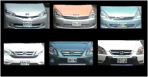
Sensors 2020, 20, 1033                                                                                   4 of 19

(b) inter-make ambiguity. In the first case, a problem occurs when different models of the same make
show similar visual appearances, as illustrated in Figure 2; i.e., the “Sentra” and “Cefiro” models of the
“Toyota” make have comparable front faces which highlights the intra-make ambiguity. In the second
case, problems arise when vehicle models of different makes have visually comparable rear/front
views, as illustrated in Figure 3; e.g., the “Toyota Camry 2005” and the “Nissan Cefiro 1999” make and
model have similar front faces, and the same trend is seen in other makes and models.

      Figure 2. Intra-make ambiguity problems between (a) Nissan Sentra 2003 and (b) Nissan Cefiro 1997;
      (c) Toyota Altis 2008 and (d) Toyota Camry 2008; and (e) Toyota Altis 2006 and (f) Toyota Camry 2006
      in the NTOU-MMR dataset. Intra-make ambiguity results when different vehicles (models) from the
      same company (make) have a comparable shape or appearance.

      Figure 3. Inter-make ambiguity problems between (a) Toyota Camry 2005 and (b) Nissan Cefiro 1999;
      (c) Toyota Tercel 2005 and (d) Nissan Sentra 2003; and (e) Toyota Camry 2006 and (f) Ford Mondeo
      2005 in the NTOU-MMR dataset. The inter-make ambiguity problem refers to the case where different
      vehicles (models) manufactured by different companies (makes) can have comparable appearances
      or shapes.

      To overcome the above-mentioned problems in VMMR, this paper presents:

•     An evaluation of different combinations of feature keypoint detectors and the HOG descriptor for
      feature extraction from vehicle images.
•     A global dictionary building scheme to tackle the ambiguity and multiplicity problems for
      vehicle make and model recognition. The optimal size of the dictionary is investigated by a series
      of experiments.
•     An evaluation of a previously unexplored approach, “bag of expressions,” for VMMR. On the
      basis of BoE, a multiclass linear SVM classifier was trained for classification. Contributions to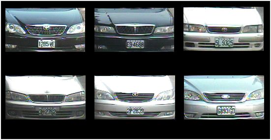
Sensors 2020, 20, 1033 5 of 19
VMMR work include learning visual words from a specific class with BoE features enhancement
and an improvement in performance.
The superiority and effectiveness of the bag of expression approach for vehicle make and model
recognition over the state-of-the-art methods are tested on random training-testing dataset splittings
of the NTOU-MMR dataset [18].
2. Proposed Methodology
This paper proposes and evaluates an up till now unexplored approach for VMMR based on BoE
and multiclass linear SVM. The key phases of the approach are as follows: (1) feature point extraction
(using the KAZE (according to its originators a Japanese word that means wind [35]), SURF (Speeded
Up Robust Features), FAST (Features from Accelerated Segments Test) and BRISK (Binary Robust
Invariant Scalable Keypoints) feature detectors), (2) HOG-based description, (3) BoE-based feature
representation and (4) linear SVM-based classification. The main focus of this work is on the frontal
view of the vehicle for make and model recognition, because other parts, such as a hood or windshield,
could mislead the classifier due to fewer variations across different vehicle makes and models. This is
a typical approach in the literature.
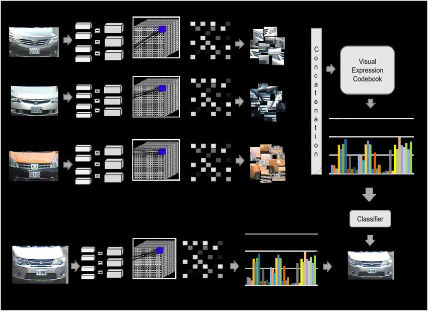
The summary of the proposed VMMR approach is presented in Figure 4. In the training phase,
features are first extracted from labeled images with specific vehicle class labels as L = {l1 , l2 , l3 ...l j },
where j is the total number of vehicle classes. During the next phase, a visual expression codebook
is generated by defining visual words. A histogram of expressions is generated by counting the
occurrences of every expression for the training images of a vehicle. Finally, a BoE-based representation
of training images is applied for the training of a supervised classifier. During the testing phase,
a feature representation is acquired for unlabeled vehicle images and quantized using a codebook of
a visual expression generated in the training phase. Then, occurrences of each expression are added
to build a histogram of expressions which is then passed to the trained classifier to detect the vehicle
label. A more detailed explanation of these processes is given in the following subsections.
Figure 4. Bag of expressions-based framework for vehicle make and model recognition (VMMR).
Sensors 2020, 20, 1033                                                                                  6 of 19

2.1. Feature Points Detection
     Different types of feature point detectors are applied to detect the unique feature points from each
class of vehicle, as shown in Figure 5. In this work, the KAZE feature detector [35] has been used to
detect feature points of interest from vehicle images. To detect the points of interest, the results of the
scale-normalized determinant of the Hessian were calculated at different numbers of scale levels.

                                       L Hessian = σ2 ( L x xLy y − L2x y)                                 (1)

where L x x are the second order horizontal derivatives, Ly y are the second order vertical derivatives
and L x x is the second order cross derivative. From the nonlinear scale space Li the set of filtered
images is given, the response of the detector was analyzed at different scale levels σi .

      Figure 5. Detected feature points using KAZE, FAST, BRISK and SURF feature detectors respectively.

      The FAST [36] detector has also been used in this work for feature points detection. FAST was
the first AST (accelerated segment test)-based algorithm for feature detection and it first examines the
values of the intensity function of pixels in a circle (of sixteen pixels) of radius r around the candidate
point p to decide if a candidate point p is either a corner point or not. After comparing the intensity
values of four pixels (I1 , I5 , I9 , I1 3) with the intensity of the candidate point p, if three of these four
pixels meet the threshold criteria, then the candidate point p is selected as an interest point (corner).
Conversely, if three of these four-pixel values are not above or below the intensity of candidate point
p plus a threshold, then the candidate point p will not be a corner point. If they are above or below,
then all sixteen pixels are examined. In this scenario at least twelve pixels should fall within the given
criterion. The process is repeated for all remaining pixels of the image.
      The BRISK [37] feature detector has also been studied here. BRISK is a binary descriptor,
based on a FAST detector that makes computations directly on image patches. It includes three parts:
(a) sampling pattern, (b) sampling pairs and (c) orientation compensation. BRISK uses a sampling
pattern surrounding keypoints on a set of concentric circles to identify whether the points are corners
in FAST or not. Then pairs are divided into two subsets, long distance and short distance pairs.
For rotation invariance, the sum of a locally computed gradient is used between short distance and
long distance pairs.
      Finally, the SURF [24] detector has also been tested. The SURF detector is capable of producing
interest points which are scale and rotation invariant. For keypoint detection, it uses integral images
and a 2D Haar wavelet. SURF uses the sum of the 2D Haar wavelet response to find the keypoint
detection around the region of interest. A Hessian matrix approximation is used to estimate the
operators of Gaussian derivatives. The Haar wavelet approximation can be computed effectively
on integral images without considering scale factor. For accurate localization of multiscale SURF
features, interpolation is required. Because of the blob-like structure, its performance is dependent on
non-maximal-suppression of the determinants of the Hessian matrices. A multiscale SURF features
interpolation is essential for accurate localization.

2.2. Description of Features
     The HOG descriptor was proposed by Dalal and Triggs [38]. It is applied after the extraction
of keypoints, as described above, from the vehicle images. The descriptor was initially used for the
detection of pedestrians from static images and it works by finding the frequency of gradient directions
from the localized region in the input image. This image is divided into grid-like patterns to get local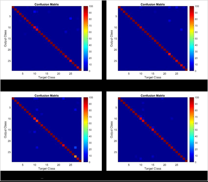
Sensors 2020, 20, 1033                                                                                           7 of 19

regions. It can represent the appearances and shapes of different objects from images with the help
of gradient direction distributions. These distributions are computed by dividing the input image
into grid-like patterns and then finding the gradient directions and gradient magnitudes from each
grid pattern of the image. The histogram of gradients is formed by computing the gradient directions
from each cell of grid in range of 0 to 180 degrees. The number of bins in the histogram is usually
nine, each corresponding to 20 degrees intervals. For each pixel in the given cell, the magnitude of
its gradient is added to a histogram bin as per the gradient direction. The histograms from these
individual cells are then combined into 2 × 2 cells and concatenated into bigger blocks. The overall
size of the HOG feature descriptor becomes 36 with four cells, each having a dimension of nine.
The descriptor size is dependent on the resolution of the image, block size and cell size. Furthermore,
to account for variations in brightness and contrast, each block of a histogram is normalized.

2.3. Generation of Visual Expressions
     For a given set of vehicle classes, the aim is to learn a global representation for the vehicle
classes by means of singular dictionary generation. The obtained features are characterized as
follows: F = { f 1 , f 2 , f 3 , . . . . . . , f j } where j represents the number of vehicle classes. The clusters
are formed by applying the widely used k-means clustering algorithm [39] on the obtained features,
and distinctive visual words are obtained for all the vehicle classes. The centroids obtained by
k-means represent the visual words which are denoted by W. The visual vocabulary is represented as
W = {W1 , W2 , W3 , . . . . . . , Wn } where W is a complete set of visual words for all the vehicle classes and
n represents a total number of visual words. Each visual word from W is paired with its N nearest
neighbors and forms an expression representation Expi , as shown in Figure 6.

      Figure 6. Visual expression generation (for illustrative purposes N has been set to 2 and only one visual
      word is considered).

     For each visual word Wi in a visual vocabulary W, we intend to find neighboring features that are
closest to the visual word. These neighboring features are computed using a distance measure such as
euclidean or Mahalanobis. In Figure 6, let us assume that the arrows denote distance, W1 represents
the visual word and that f 1 , f 2 , f 3 , . . . . . . , f 5 represent the features considering N = 2; i.e., two nearest
neighbors. The expression [ Exp]i is formed by finding the closest features to the visual word. In this
case, W1 is nearest to two features [ f ]1 and [ f ]2 . Therefore, W1 is combined with [ f ]1 and [ f ]2 by finding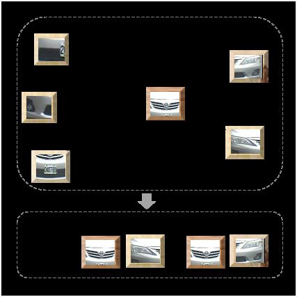
Sensors 2020, 20, 1033                                                                                   8 of 19

the mean of each pair (W1 , [ f ]1 ) and (W1 , [ f ]2 ). These pairs are stacked together and added into a
visual expression codebook. The process is repeated for the remaining visual words; thus, the final
expression codebook contains the mean pairs (Wi , [ f ]i ) for each visual word.
      For each of these visual words w, the neighboring features are computed through a distance
measure to form an expression dictionary. In experimentation, different distance measures have been
used for distance calculation, such as Mahalanobis and euclidean distances. The Mahalanobis distance
is calculated as follows:                      q
                                       Dω µ = ( ω − µ ) S − 1 ( ω − µ ) t                              (2)

where S− 1 represents the inverse covariance matrix, ω represents a visual word and µ represents the
feature distribution. The euclidean distance is given by the well-known expression
                                                    q
                                          Dω µ =        (ω − µ)(ω − µ)t                                     (3)

     Neighboring features are described in terms of independent pairs. These pairs are combined
with the visual words irrespective of their relationship with other visual words. For example, a visual
word having 10 neighboring features will be paired with each one to form 10 expressions. This offers
some degree of view independent representation which is tolerant of occlusion. Thus, the achieved
representation in terms of expressions provides discriminative power to word pairs to discard
information relevant to other visual words and recognize the vehicle classes even in an occluded
environment. The problem of view independence is addressed by forming a vector of frequency counts
of expressions for each vehicle class. These vectors help in differentiating different makes and models.
The expressions formed through visual word pairs are represented as follows:

                                Exp1 = {exp1 1, exp1 2, exp1 3, . . . . . . , exp1 N }
                                Exp2 = {exp2 1, exp2 2, exp2 3, . . . . . . , exp2 N }
                                Exp3 = {exp3 1, exp3 2, exp3 3, . . . . . . , exp3 N }                      (4)
                                  ...
                                Expz = {expz 1, expz 2, expz 3, . . . . . . , expz N }

where N represents the number of nearest neighboring features combined to form an expression.
Furthermore, these expressions are combined together to form an expression dictionary
E = { Exp1 , Exp2 , Exp3 , . . . . . . , Expz } where z is the total number of expressions. The nearest features
combined with visual words are expected to vary distinctively with respect to each class; hence,
the formed expressions are discriminative enough to distinguish between different classes.

2.4. Histogram of Expressions
     Histograms of expressions are generated by computing the frequency of occurrence of each given
expression from each of the feature vectors of the image. This mapping of features to neighboring
expressions is computed through a distance measure; e.g., euclidean distance or Mahalanobis distance.
The histogram of expressions for vehicle images acts as the training or testing sample to be used
in classification. The histograms of expressions displayed in Figure 7 belong to some of the vehicle
samples taken from different classes of NTOU-MMR dataset. These are used as training and testing
data for a classifier. The frequency of expressions varies for each class of the dataset which helps in
differentiating different vehicle classes.
Sensors 2020, 20, 1033 9 of 19
Figure 7. Histograms of expressions for the NTOU-MMR dataset (random sample of each specified
vehicle class).
2.5. Classification
The identification of a vehicle manufacturer and model is an essential task when designing a
VMMR system. The well-known multiclass linear SVM classifier for the classification of vehicle make
and model has been applied. This procedure learns β and β( β − 1)/2 binary SVMs, where β represents
the total number of unique vehicle classes by applying one-versus-all and all-pairs coding design
models respectively. By applying a sparse-random coding design model, this procedure learns random
(but approximately 15 log2 β) binary SVMs. Different SVM parameters are chosen to achieve good
recognition accuracy, as further discussed in the experimental discussion and results section below.
3. Experimental Results and Discussion
To investigate the efficiency and effectiveness of the BoE-based approaches for VMMR,
the proposed approach has been evaluated on the publicly available NTOU-MMR dataset [18], as it
serves as a good benchmark dataset for performance comparison among different VMMR works.
This dataset was published in the relevant work of VMMR [3] and has been gathered under the
Vision-based Intelligent Environment (VBIE) project [18]. The original dataset was captured in different
environmental conditions and then the whole dataset was divided into a training image set and
testing images set. The training images set contains 2846 vehicle images, and the testing set contains
3793 vehicle images. There are 29 different classes in the dataset. The set of make-model classes
in NTOU-MMR dataset is: class number one (C1) Toyota Altis, C2 Toyota Camry, C3 Toyota Vios,
C4 Toyota Wish, C5 Toyota Yaris, C6 Toyota Previa, C7 Toyota Innova, C8 Toyota SURF, C9 Toyota
Tercel, C10 Toyota RAV, C11 Honda CRV, C12 Honda Civic, C13 Honda Fit, C14 Nissan March,
C15 Nissan Livna, C16 Nissan Teana, C17 Nissan Sentra, C18 Nissan Cefiro, C19 Nissan Xtrail, C20
Nissan Tiida, C21 Mitsubishi Zinger, C22 Mitsubishi Outlander, C23 Mitsubishi Savrin, C24 Mitsubishi
Lancer, C25 Suzuki Solio, C26 Ford Liata, C27 Ford Escape, C28 Ford Mondeo and C29 Ford Tierra.
The dataset contains the images of the vehicles captured from different viewing angles in a range
between −20◦ to +20◦ and in different weather conditions; for example, cloudy, rainy and sunny.
Images of the dataset were also captured at night time, day time and under different illumination
conditions. In addition, there are a few images of vehicles occluded by other objects, such as anSensors 2020, 20, 1033 10 of 19
umbrella, pedestrians and another vehicle. Some of the challenging scenarios in this dataset are shown
in Figure 8.
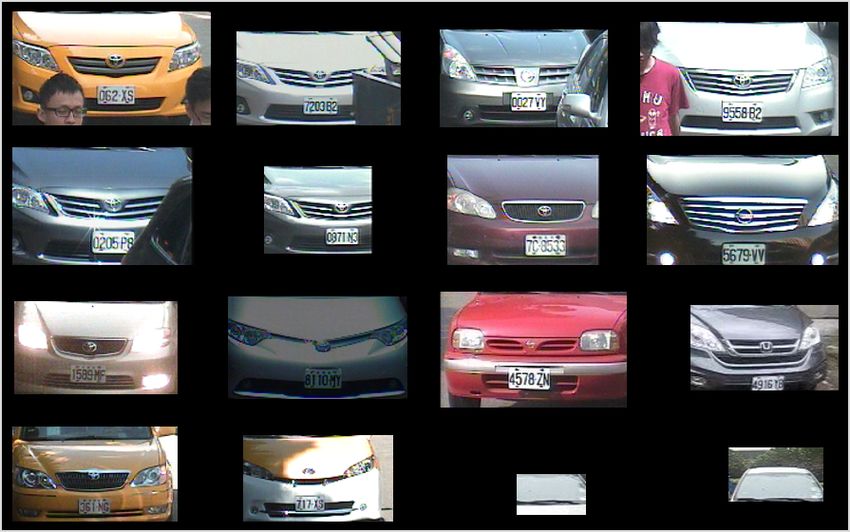
Figure 8. Some of the challenging scenarios in the NTOU-MMR dataset. The BoE-based approaches
were successful in predicting the make–model class in all of the above cases except the last two
(noisy images).
There are some issues with the NTOU-MMR dataset: (1) duplication of images: in some classes,
duplicated images of a vehicle saved with a different label; (2) misplacement of images: various class
directories contain the vehicles of other classes; (3) biased division of testing and training images: the
strategy for how to divide the data for each class into training and testing is not clear, but any division
can affect the performance of the system; (4) noisy data: some vehicle image samples are noisy and
also contain irrelevant data for processing. All the experiments reported here were performed on Intel
CoreTM i7-4600M CPU (2.90 GHz) 8 GB RAM, using MATLAB. Similar to prior VMMR work [25],
for evaluation purposes we have used a hold-out cross validation scheme for the dataset [18] to build
dissimilar training and testing splits for all vehicle classes. Ten such training and testing splits are built,
and the mean accuracy of these splits is reported. For every split of the data set, randomly, 20% of
vehicle images are picked for testing purposes and the other 80% of the vehicle images are used to
train the algorithm—referred to as 80–20 NTOU-MMR splits. These proportions are commonly used
by other researchers using this dataset. For each split, the division criteria for a number of images
for training (#Train) and testing (#Test) sets are similar to [25]. Processing speed and mean accuracy
are obtained by averaging results for every split. Results have also been evaluated with 70–30 and
60–40 splits .
3.1. Selection of Optimal Parameters
Using the 80–20 NTOU-MMR Datasets, optimized parameters for each phase were obtained
by cross-validation. Here, the best results mean the best trade-off between average accuracy and
processing speed.
3.1.1. Dictionary Size
In the dictionary building phase, dictionary size (the number of clusters) affects the overall
performance of the VMMR module in the context of processing speed and accuracy. For the KAZE
HOG feature descriptor, dictionary size was varied from 100 to 1000 and the best results were achieved
for dictionary size 350, as shown in Table 1. For the other combinations, dictionary size was varied
in the range 100 to 3000, and it was found that the best trade-offs between accuracy and speed forSensors 2020, 20, 1033 11 of 19
dictionary size were 1200 for BRISK HOG, 2200 for SURF HOG and 1500 for FAST HOG, as presented
in Table 2.
Table 1. Impact of varying dictionary size on average accuracy with the KAZE feature detector
(using Mahalanobis and sparse-random combination).
Dictionary Size 100 200 300 350 400 500 600 700 1000
KAZE_HOG _ BoE 93.03 96.36 97.93 98.22 98.39 98.58 98.74 98.88 99.01
Table 2. Impact of varying dictionary size on average accuracy with FAST, BRISK and SURF feature
detectors (using Mahalanobis and sparse-random combination).
Dictionary Size FAST_HOG_BoE SURF_HOG_BoE BRISK_HOG_BoE
100 90.56% 86.54% 91.65%
500 96.67% 93.68% 97.59%
1000 97.56% 95.93% 98.21%
1200 97.94% 96.11% 98.43%
1500 98.33% 96.26% 98.76%
2000 98.65% 97.08% 98.94%
2200 98.73% 97.24% 99.06%
2500 98.78% 97.66% 99.09%
3000 98.86% 97.71% 99.14%
3.1.2. BoE Parameters
Optimization of BoE parameters involves some different parameters: Which distance measure is
used for distance calculation and the number of nearest neighbors N for the formation of expression
codebook. The number of nearest neighbors N was varied from 0 to 5 and the best results were
obtained with N = 2, as shown in Figure 9. Euclidean and Mahalanobis distance measures were tested
for codebook generation.
Figure 9. Average accuracy with respect to number of neighbors N for visual expression codebook
creation for the NTOU-MMR dataset using the sparse-random coding model and Mahalanobis distance.
3.1.3. SVM Parameters
Finally, optimized classifier parameters were obtained on the basis of optimal dictionary sizes.
In the classification phase, the multiclass linear SVM classifier was applied with the following
parameters: a linear kernel function; an automatic kernel scale; a size of box constraint set to 29;
fit posterior and standardize enabled. Three different coding design models were used (one-vs.-all,
sparse-random and all-pairs).Sensors 2020, 20, 1033 12 of 19
3.2. Performance Evaluation
Different experiments were carried out to study the effects of parameters to aim for an efficient
VMMR framework. SURF-based BoE obtains 95.44% average accuracy with a processing speed 11.0 fps.
KAZE-based BoE achieves 96.76% average accuracy and 16.6 fps. As explained earlier, different
dictionary sizes were explored. Although the best accuracy is achieved with a larger dictionary size,
computation time is sacrificed to the point where it is not suitable for real-time applications. Therefore,
dictionary size was chosen to maintain reasonable speeds. For example, for KAZE HOG the approach
was tested with dictionary sizes from 100 to 1000 (Table 1), obtaining 93.03% average accuracy with
size 100 and 99.01% with size 1000. For the best trade-off between average accuracy and processing
speed, a dictionary size of 350 was chosen, achieving average accuracy of 98.22%. For the FAST
HOG, BRISK HOG and SURF HOG feature descriptors, dictionary size was varied from 100 to 3000
(Table 2); choosing a size of 1500, for example, for FAST HOG, achieves 98.33% average accuracy
(even if with a size of 3000 and average accuracy of 98.86% is reached). For SURF HOG a best result of
97.24% was obtained with a dictionary size of 2200. For BRISK HOG, for the best trade-off between
average accuracy and processing speed, a dictionary size of 1200 was chosen, achieving 98.43% average
accuracy. Experiments with different validation splits were performed and are presented in Table 3.
From these experiments, it can be concluded that the approach performs well also for the additional
70–30 and 60–40 splits.
Table 3. Impact of validation splits on average accuracy for KAZE, FAST, BRISK and SURF
(using Mahalanobis and sparse-random combination).
Average Accuracy % with Validation Scheme
Mahalanobis + Mahalanobis + Mahalanobis +
Feature Extraction sparse-random sparse-random sparse-random
60–40 70–30 80–20
KAZE _350 97.75% 97.97% 98.22%
HOG
FAST_ 1500 + 97.03% 97.66% 98.33%
SURF _2200 BoE 96.84% 97.09% 97.24%
BRISK _1200 97.60% 98.08% 98.43%
Table 4. Results of bag of expressions-based VMMR approach with the different coding design models.
Average Accuracy % with Coding Design
Feature Extraction Distance Measure
One-vs.-all All-pairs Sparse-random
Mahalanobis 98.27% 98.00% 98.22%
KAZE_350
Euclidean 98.19% 97.83% 98.18%
HOG Mahalanobis 98.22% 97.09% 98.33%
FAST_1500
+ Euclidean 98.36% 96.85% 98.21%
BoE Mahalanobis 97.15% 96.32% 97.24%
SURF_2200
Euclidean 97.32% 96.41% 97.19%
Mahalanobis 98.49% 97.37% 98.43%
BRISK_1200
Euclidean 98.35% 97.66% 98.25%
Different combinations of distance measure and coding design model were evaluated with
KAZE HOG, FAST HOG, BRISK HOG and SURF HOG, as presented in Table 4. In the case of
KAZE HOG ( dictionary size = 350), the highest average accuracy (98.27%) was obtained with
one-vs.-all and Mahalanobis, but processing speed was worse compared to the sparse-random and
Mahalanobis combination. The same descriptor with all-pairs results in less accuracy as well as slowerSensors 2020, 20, 1033 13 of 19
processing speed compared to other combinations. Its best result (best trade-off between speed and
accuracy) is 98.22% average accuracy using sparse-random and Mahalanobis combination. FAST HOG
(dictionary size = 1500), with one-vs.-all and euclidean results in the highest average accuracy (98.36%),
but it is computationally slow compared to sparse-random. The best trade-off results (98.33%) are
obtained using a combination of sparse-random and Mahalanobis with dictionary size 1500. For SURF
HOG feature descriptor (dictionary size = 2200), its highest accuracy is 97.32%, using euclidean
and sparse-random, but at the expense of computational speed. The best trade-off performance is
achieved using a sparse-random and Mahalanobis distance combination, reaching 97.24%. BRISK
HOG (dictionary size = 1200), reaches its highest average accuracy at 98.49% using one-vs.-all and
Mahalanobis, but again sacrificing speed. Its best trade-off result is 98.43% using Mahalanobis and
sparse-random combination. The average per-class accuracies of the proposed approaches on the
NTOU-MMR dataset are presented in Table 5, which illustrates the class-wise dominance of the
proposed approaches on NTOU-MMR dataset.
Table 5. The average per-class accuracy of the proposed approaches on the NTOU-MMR dataset.
The last column shows the mean average precision of vehicle classes.
Method C1 C2 C3 C4 C5 C6 C7 C8 C9 C10 C11
KAZE_350 99.6 99.4 98.4 99.1 100 97.9 99.3 99.7 100 90.8 90.4
HOG
FAST_1500 + 99.4 100 97.8 100 99.8 100 100 99.5 100 94.6 99.6
SURF_2200 BoE 98.1 100 97.9 99.6 100 99.7 99.4 98.5 100 87.5 82.4
BRISK_1200 99.1 100 99.6 100 100 100 98.7 98.3 100 90.8 89.6
Method C12 C13 C14 C15 C16 C17 C18 C19 C20 C21 C22
KAZE_350 100 100 99.7 99.4 98.5 99.3 99.8 100 99.5 99.2 99.7
HOG
FAST_1500 + 100 100 100 99.6 98.4 99.4 99.7 99.5 100 99.7 86.7
SURF_2200 BoE 100 96.9 100 100 99.6 99.8 100 100 99.7 100 91.2
BRISK_1200 100 100 100 89.8 98.4 100 100 95.6 100 100 99.6
Method C23 C24 C25 C26 C27 C28 C29 Average per-class Accuracy
KAZE_350 95.7 100 89.6 99.6 99.4 94.4 100 98.22%
HOG
FAST_1500 + 99.6 99.7 90.9 99.5 91.9 96.3 100 98.33%
SURF_2200 BoE 100 100 99.3 100 73.9 95.6 100 97.24%
BRISK_1200 96.1 100 99.7 100 99.7 99.5 100 98.43%
The performance of the approach presented here is also illustrated by means of confusion matrices
and ROC curves, as shown in Figures 10 and 11 respectively. The problem of multiplicity, as discussed
in Figure 1, was resolved by applying the proposed approaches. For example, C4 had a multiplicity
problem that did not degrade the results, as can be seen in Table 5. The multiplicity problem in C11
(Honda CRV) did not significantly affect the FAST HOG-based BOE approach. However, KAZE,
SURF and BRISK degrade somewhat to 90.4%, 82.4% and 89.6% average accuracy. The inter-make
ambiguity problems between C2 and C18; C9 and C17; and C2 and C28, as shown in Figure 3, were also
addressed. The intra-make ambiguity problems between C17 and C18; C1 and C2; and C1 and C2,
as shown in Figure 2, were also overcome. The results for all these ambiguous classes show good
performance, as can be seen in Table 5. Furthermore, these good performance indicators show that the
proposed approach is able to cope well with many of the challenges in this dataset (as illustrated by
Figure 8).Sensors 2020, 20, 1033 14 of 19
3.3. Computational Cost
The proposed approach not only results in higher accuracy but also good time performance,
to levels suitable for real-time operation compared to state-of-the-art work, even with relatively modest
hardware (please see Table 6). For example, in our case, KAZE HOG with a dictionary size of 350,
achieved an average accuracy of 98.22% with a processing speed 24.7 fps. FAST with a dictionary
size of 1500, obtains a processing speed of 15.4 fps with an average accuracy of 98.33%. SURF with
a dictionary of size 2200, has an average accuracy of 97.24% with 18.6 fps. Finally, BRISK with a
dictionary size of 1200, achieves 6.7 fps with the highest average accuracy of 98.43%.
Figure 10. Confusion matrices for bag of expression for the 80–20 NTOU-MMR dataset.Sensors 2020, 20, 1033 15 of 19
Figure 11. ROC curves for bag of expression for 80–20 NTOU-MMR dataset.
3.4. Comparison with State-Of-The-Art
The proposed BoE-based approaches for a vehicle make and model recognition presented in
this paper outperform numerous related VMMR works, both in terms of classification accuracy and
processing speed. Accuracy and speed comparisons are presented in Table 6. Hardware used in other
works, where known, is also given. The table provides comprehensive results on NTOU-MMR and
other VMMR datasets. It is pertinent to mention that other datasets are quite similar to NTOU-MMR
in terms of environment and some of the challenges discussed earlier. Furthermore, all these methods
mainly focus on frontal view of vehicles for VMMR. The performance and computational cost of [18]
on the NTOU-MMR dataset are not sufficient for real-time VMMR. The processing speed of [20,23,30]
is not up-to-the-mark for a real-time environment. The accuracy obtained from these works is also
not high enough for a high performance VMMR system. The performance of [31,32] is sufficient for
VMMR work but the authors do not discuss the computational cost in their work. The performance
and computational cost of [40,41] are sufficient for VMMR work but less than what has been presented
here. The work proposed in [42] does not provides satisfactory results on the NTOU-MMR dataset.
The performance and computational cost of [25,33] on the NTOU-MMR dataset are acceptable but far
behind from the proposed approach in terms of average accuracy and processing speed. Therefore,
it can be concluded from Table 6 that the BoE-based VMMR procedure is superior in the context of
performance and computational cost.Sensors 2020, 20, 1033 16 of 19
Table 6. Comparison with state-of-the-art work.
Average Speed
Work/Hardware Features Classification Dataset
Accuracy (fps)
Baran et al.
[20] (2015)
CPU—Dual Core 3859 vehicle
SURF, SIFT, Multi-class 91.70% 30
i5 650 CPU images with
Edge-Histogram SVM 97.20% 0.5
3200 MHz 2GB RAM 17 classes
Win. Server 2008 R2
Enterprise (64-bit).
He et al. 1196 vehicle
Multi-scale Artificial
[23] (2015) images and 92.47% 1
retinex Neural Network
Hardware unknown 30 classes
Tang et al.
223 vehicle
[30] (2017) Local Gabor Nearest
images with 91.60% 3.3
i7 3.4GHz, 4GB RAM Binary Pattern Neighborhood
8 classes
Quadro 2000 GPU
Nazemi et al.
[40] (2018) A fine-grained Iranian on-road
Dense-SIFT 97.51% 11.1
3.4 GHz Intel CPU classification vehicle dataset
32 GB RAM
Jie Fang et al.
44,481 vehicle
[31] (2017) Convolution
images with 98.29% –
ı7-4790K CPU Neural Network
281 classes
TITAN X GPU
Afshin Dehghan 44,481 vehicle
Convolution
et al. [32] (2017) images with 95.88% –
Neural Network
TITAN XP GPUs 281 classes
Hyo Jong et al.
291,602 vehicle
[41] (2019) Residual
images with 96.33% 9.1
i7-4790 CPU 3.6GHz Squeeze Net
766 classes
GTX 1080 GPU
Chen et al.
Symmetric Sparse representation
[18] (2015) NTOU-MMR 91.10% 0.46
SURF and hamming distance
Hardware unknown
Manzoor et al.
[42] [2017) SIFT SVM NTOU-MMR 89.00% –
i7 3.4GHz 16GB RAM
Jabbar et al.
[25] (2016) Single and ensemble
SURF NTOU-MMR 94.84% 7.4
i5 CPU 2.94GHz of multi-class SVM
16GB RAM
Manzoor et al.
Random Forest 94.53% 35.7
[33] [2019) HOG NTOU-MMR
SVM 97.89% 13.9
i7 3.4GHz 16GB RAM
Our KAZE_350 98.22% 24.7
HOG
Approach FAST_1500 98.33% 15.4
+ Linear SVM NTOU-MMR
i7-4600M CPU SURF_2200 97.24% 18.6
BoE
2.90GHz 8GB RAM BRISK_1200 98.43% 6.7
4. Conclusions
This paper has presented a new BoE-based approach for the recognition of vehicle make and
model with a higher degree of accuracy which is also suitable for real-time ITS applications. This work
has determined, from the quality measures, that the KAZE HOG-based BoE combination is more
suitable for a real-time VMMR environment. An expressions-based global dictionary building schemeSensors 2020, 20, 1033 17 of 19
has been studied to address the multiplicity and ambiguity problems in VMMR. From experimental
evaluations, optimal sizes for the dictionaries have been recommended. Optimal parameter selection
and evaluation of SVM classification has proven useful for real-time VMMR.
The superiority and effectiveness of the BoE-based approach over the state-of-the-art methods
have been validated using random training-testing splits of the NTOU-MMR Dataset. Although the
proposed approaches achieved good performances, we plan to explore more robust features in the
future that are applicable for real-time VMMR. We will also explore further an encoding scheme and a
classification scheme. Likewise, the learning approach also needs to be enhanced when unseen vehicle
models are included in the dataset. We will also explore different schemes of ROI (Region of Interest)
utilization and division. We also have a plan to build a general VMMR dataset for VMMR work which
satisfies the requirements of the standard benchmark dataset. Exploring deep learning features from a
pretrained network instead of HOG with a bigger dataset is also in line for future work.
Author Contributions: Methodology, software, validation, investigation, visualization, writing-original draft
preparation, A.A.J.; Software, investigation, A.M.B.; Conceptualization, supervision, writing-review, editing,
project administration, funding acquisition F.H., M.H.Y. and S.A.V. All authors have read and agree to the
published version of the manuscript.
Funding: Muhammad Haroon Yousaf received funding from the Higher Education Commission, Pakistan
for Swarm Robotics Lab under the National Centre for Robotics and Automation (NCRA). The authors
also acknowledge support from the Directorate of ASR& TD, University of Engineering and Technology
Taxila, Pakistan.
Conflicts of Interest: The authors declare no conflict of interest.
References
1. Pearce, G.; Pears, N. Automatic make and model recognition from frontal images of cars. In Proceedings
of the 2011 8th IEEE International Conference on Advanced Video and Signal Based Surveillance (AVSS),
Klagenfurt, Austria, 30 August–2 September 2011; pp. 373–378.
2. Sivaraman, S.; Trivedi, M.M. Looking at vehicles on the road: A survey of vision-based vehicle detection,
tracking, and behavior analysis. IEEE Trans. Intell. Transp. Syst. 2013, 14, 1773–1795. [CrossRef]
3. Hsieh, J.W.; Chen, L.C.; Chen, D.Y. Symmetrical SURF and its applications to vehicle detection and vehicle
make and model recognition. Trans. Intell. Transp. Syst. 2014, 15, 6–20. [CrossRef]
4. Tsai, L.W.; Hsieh, J.W.; Fan, K.C. Vehicle detection using normalized color and edge map. IEEE Trans. Image
Process. 2007, 16, 850–864. [CrossRef] [PubMed]
5. Wang, S.; Cui, L.; Liu, D.; Huck, R.; Verma, P.; Sluss, J.J.; Cheng, S. Vehicle Identification Via Sparse
Representation. IEEE Trans. Intell. Transp. Syst. 2012, 13, 955–962. [CrossRef]
6. Kim, Z.; Malik, J. Fast vehicle detection with probabilistic feature grouping and its application to vehicle
tracking. In Proceedings of the Ninth IEEE International Conference on Computer Vision, Nice, France,
13–16 October 2003.
7. Kumar, T.S.; Sivanandam, S. A modified approach for detecting car in video using feature extraction
techniques. Eur. J. Sci. Res. 2012, 77, 134–144.
8. Betke, M.; Haritaoglu, E.; Davis, L.S. Real-time multiple vehicle detection and tracking from a moving
vehicle. Mach. Vis. Appl. 2000, 12, 69–83. [CrossRef]
9. Gu, H.Z.; Lee, S.Y. Car model recognition by utilizing symmetric property to overcome severe pose variation.
Mach. Vis. Appl. 2013, 24, 255–274. [CrossRef]
10. Hoffman, C.; Dang, T.; Stiller, C. Vehicle detection fusing 2D visual features. In Proceedings of the IEEE
Intelligent Vehicles Symposium, Parma, Italy, 14–17 June 2004.
11. Leotta, M.J.; Mundy, J.L. Vehicle surveillance with a generic, adaptive, 3d vehicle model. IEEE Trans. Pattern
Anal. Mach. Intell. 2010, 33, 1457–1469. [CrossRef]
12. Guo, Y.; Rao, C.; Samarasekera, S.; Kim, J.; Kumar, R.; Sawhney, H. Matching vehicles under large pose
transformations using approximate 3d models and piecewise mrf model. In Proceedings of the 2008 IEEE
Conference on Computer Vision and Pattern Recognition, Anchorage, AK, USA, 23–28 June 2008; pp. 1–8.Sensors 2020, 20, 1033 18 of 19
13. Hou, T.; Wang, S.; Qin, H. Vehicle matching and recognition under large variations of pose and illumination.
In Proceedings of the 2009 IEEE Computer Society Conference on Computer Vision and Pattern Recognition
Workshops, Miami, FL, USA, 20–25 June 2009.
14. Faro, A.; Giordano, D.; Spampinato, C. Adaptive background modeling integrated with luminosity sensors
and occlusion processing for reliable vehicle detection. IEEE Trans. Intell. Transp. Syst. 2011, 12, 1398–1412.
[CrossRef]
15. Jazayeri, A.; Cai, H.; Zheng, J.Y.; Tuceryan, M. Vehicle detection and tracking in car video based on motion
model. IEEE Trans. Intell. Transp. Syst. 2011, 12, 583–595. [CrossRef]
16. Rojas, J.C.; Crisman, J.D. Vehicle detection in color images. In Proceedings of the Conference on Intelligent
Transportation Systems, Boston, MA, USA,12 November 1997.
17. Guo, D.; Fraichard, T.; Xie, M.; Laugier, C. Color modeling by spherical influence field in sensing driving
environment. In Proceedings of the IEEE Intelligent Vehicles Symposium 2000 (Cat. No. 00TH8511),
Dearborn, MI, USA, 5 October 2000.
18. Chen, L.C.; Hsieh, J.W.; Yan, Y.; Chen, D.Y. Vehicle make and model recognition using sparse representation
and symmetrical SURFs. Pattern Recognit. 2015, 48, 1979–1998. [CrossRef]
19. Lowe, D.G. Distinctive image features from scale-invariant keypoints. Int. J. Comput. Vis. 2004, 60, 91–110.
[CrossRef]
20. Baran, R.; Glowacz, A.; Matiolanski, A. The efficient real-and non-real-time make and model recognition of
cars. Multimedia Tools Appl. 2015, 74, 4269–4288. [CrossRef]
21. Fraz, M.; Edirisinghe, E.A.; Sarfraz, M.S. Mid-level-representation based lexicon for vehicle make and
model recognition. In Proceedings of the 22nd International Conference on Pattern Recognition, Stockholm,
Sweden, 24–28 August 2014.
22. Manzoor, M.A.; Morgan, Y. Vehicle make and model recognition using random forest classification for
intelligent transportation systems. In Proceedings of the 8th Annual Computing and Communication
Workshop and Conference (CCWC), Las Vegas, NV, USA, 8–10 January 2018.
23. He, H.; Shao, Z.; Tan, J. Recognition of car makes and models from a single traffic-camera image. IEEE Trans.
Intell. Transp. Syst. 2015, 16, 3182–3192. [CrossRef]
24. Bay, H.; Ess, A.; Tuytelaars, T.; Van Gool, L. Speeded-up robust features (SURF). Comput. Vision Image
Understanding 2008, 110, 346–359. [CrossRef]
25. Siddiqui, A.J.; Mammeri, A.; Boukerche, A. Real-time vehicle make and model recognition based on a bag of
SURF features. IEEE Trans. Intell. Transp. Syst. 2016, 17, 3205–3219. [CrossRef]
26. Nazir, S.; Yousaf, M.H.; Nebel, J.C.; Velastin, S.A. Dynamic Spatio-Temporal Bag of Expressions (D-STBoE)
model for human action recognition. Sensors 2019, 19, 2790. [CrossRef]
27. Nazir, S.; Yousaf, M.H.; Nebel, J.C.; Velastin, S.A. A Bag of Expression framework for improved human
action recognition. Pattern Recognit. Lett. 2018, 103, 39–45. [CrossRef]
28. Psyllos, A.; Anagnostopoulos, C.N.; Kayafas, E. Vehicle model recognition from frontal view image
measurements. Comput. Stand. Interfaces 2011, 33, 142–151. [CrossRef]
29. Varjas, V.; Tanács, A. Car recognition from frontal images in mobile environment. In Proceedings of
the 8th International Symposium on Image and Signal Processing and Analysis (ISPA), Trieste, Italy,
4–6 September 2013.
30. Tang, Y.; Zhang, C.; Gu, R.; Li, P.; Yang, B. Vehicle detection and recognition for intelligent traffic surveillance
system. Multimed. Tools Appl. 2017, 76, 5817–5832. [CrossRef]
31. Fang, J.; Zhou, Y.; Yu, Y.; Du, S. Fine-grained vehicle model recognition using a coarse-to-fine convolutional
neural network architecture. IEEE Trans. Intell. Transp. Syst. 2016, 18, 1782–1792. [CrossRef]
32. Dehghan, A.; Masood, S.Z.; Shu, G.; Ortiz, E. View Independent Vehicle Make, Model and Color Recognition
Using Convolutional Neural Network. Available online: https://arxiv.org/abs/1702.01721 (accessed on 10
February 2020).
33. Manzoor, M.A.; Morgan, Y.; Bais, A. Real-Time Vehicle Make and Model Recognition System. Mach. Learn.
Knowl. Extr. 2019, 1, 611–629. [CrossRef]
34. Soon, F.C.; Khaw, H.Y.; Chuah, J.H.; Kanesan, J. PCANet-based convolutional neural network architecture
for a vehicle model recognition system. IEEE Trans. Intell. Transp. Syst. 2018, 20, 749–759. [CrossRef]
35. Alcantarilla, P.F.; Bartoli, A.; Davison, A.J. KAZE features. In Computer Vision—ECCV 2012; Springer:
Berlin/Heidelberg, Germany, 2012; Volume 7577, pp. 214–227.Sensors 2020, 20, 1033 19 of 19
36. Rosten, E.; Drummond, T. Machine learning for high-speed corner detection. In Computer Vision—ECCV 2006;
Springer: Berlin/Heidelberg, Germany, 2006; Volume 3951, pp. 430–443.
37. Leutenegger, S.; Chli, M.; Siegwart, R. BRISK: Binary robust invariant scalable keypoints. In Proceedings of
the 2011 IEEE international conference on computer vision, Barcelona, Spain, 6–13 November 2011.
38. Dalal, N.; Triggs, B. Histograms of oriented gradients for human detection. In Proceedings of the 2005
IEEE Computer Society Conference on Computer Vision and Pattern Recognition, San Diego, CA, USA,
20–25 June 2005.
39. Jain, A.K. Data clustering: 50 years beyond K-means. Pattern Recognit. Lett. 2010, 31, 651–666. [CrossRef]
40. Nazemi, A.; Shafiee, M.J.; Azimifar, Z.; Wong, A. Unsupervised Feature Learning Toward a Real-time
Vehicle Make and Model Recognition. Available online: https://arxiv.org/abs/1806.03028 (accessed on
10 February 2020).
41. Lee, H.J.; Ullah, I.; Wan, W.; Gao, Y.; Fang, Z. Real-time vehicle make and model recognition with the
residual SqueezeNet architecture. Sensors 2019, 19, 982. [CrossRef]
42. Manzoor, M.A.; Morgan, Y. Vehicle Make and Model classification system using bag of SIFT features.
In Proceedings of the 7th Annual Computing and Communication Workshop and Conference (CCWC),
Las Vegas, NV, USA, 9–11 January 2017.
c 2020 by the authors. Licensee MDPI, Basel, Switzerland. This article is an open access
article distributed under the terms and conditions of the Creative Commons Attribution
(CC BY) license (http://creativecommons.org/licenses/by/4.0/).You can also read