COVID-19 induced lower-tropospheric ozone changes - eLib
←
→
Page content transcription
If your browser does not render page correctly, please read the page content below
LETTER • OPEN ACCESS

COVID-19 induced lower-tropospheric ozone changes
To cite this article: Mariano Mertens et al 2021 Environ. Res. Lett. 16 064005

View the article online for updates and enhancements.

                             This content was downloaded from IP address 129.247.247.240 on 21/05/2021 at 11:17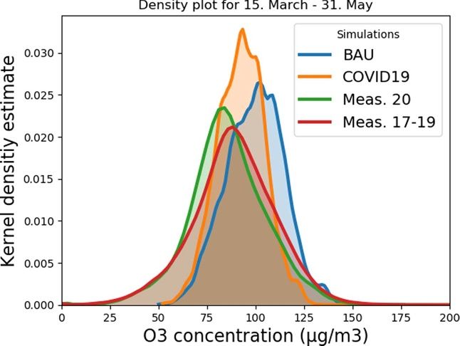
Environ. Res. Lett. 16 (2021) 064005 https://doi.org/10.1088/1748-9326/abf191
LETTER
COVID-19 induced lower-tropospheric ozone changes
OPEN ACCESS
Mariano Mertens1,∗, Patrick Jöckel1, Sigrun Matthes1, Matthias Nützel1, Volker Grewe1,2
RECEIVED
25 January 2021
and Robert Sausen1
1
REVISED
Deutsches Zentrum für Luft- und Raumfahrt, Institut für Physik der Atmosphäre, Oberpfaffenhofen, Germany
2
16 March 2021 Delft University of Technology, Faculty of Aerospace Engineering, Section Aircraft Noise and Climate Effects, Delft, The Netherlands
∗
Author to whom any correspondence should be addressed.
ACCEPTED FOR PUBLICATION
24 March 2021 E-mail: mariano.mertens@dlr.de
PUBLISHED
18 May 2021 Keywords: COVID-19, air quality, ozone, source attribution
Supplementary material for this article is available online
Original content from
this work may be used
under the terms of the
Creative Commons Abstract
Attribution 4.0 licence.
The recent COVID-19 pandemic with its countermeasures, e.g. lock-downs, resulted in decreases
Any further distribution
of this work must in emissions of various trace gases. Here we investigate the changes of ozone over Europe
maintain attribution to
the author(s) and the title associated with these emission reductions using a coupled global/regional chemistry climate
of the work, journal model. We conducted and analysed a business as usual and a sensitivity (COVID19) simulation. A
citation and DOI.
source apportionment (tagging) technique allows us to make a sector-wise attribution of these
changes, e.g. to natural and anthropogenic sectors such as land transport. Our simulation results
show a decrease of ozone of 8% over Europe in May 2020 due to the emission reductions. The
simulated reductions are in line with observed changes in ground-level ozone. The source
apportionment results show that this decrease is mainly due to the decreased ozone precursors
from anthropogenic origin. Further, our results show that the ozone reduction is much smaller
than the reduction of the total NOx emissions (around 20%), mainly caused by an increased ozone
production efficiency. This means that more ozone is produced for each emitted NOx molecule.
Hence, more ozone is formed from natural emissions and the ozone productivities of the
remaining anthropogenic emissions increase. Our results show that politically induced emissions
reductions cannot be transferred directly to ozone reductions, which needs to be considered when
designing mitigation strategies.
1. Introduction This increase is due to the complex (nonlinear)
ozone chemistry, which explains that a reduction in
The COVID-19 pandemic has a strong socio- ozone precursors can lead to increasing ozone pro-
economic impact [1]. As one consequence, in 2020 duction, if the ozone production takes place in the
reduced carbon dioxide (CO2 ) emissions from vari- ‘VOC-limited’ regime (e.g. [1, 6–9]). The emission
ous sectors have been noted in many regions world- reduction during spring 2020 related to COVID-19
wide (e.g. [2, 3]). Typically, such reductions of CO2 is a rare real-life experiment from a scientific view-
emissions are expected to be related to air quality point [1], similar to the eruption of Eyjafjallajökull in
improvements through reduced co-emission of pol- 2010, which halted air-traffic for a short period in the
lutants. Indeed, reductions of particulate matter and affected regions (e.g. [10, 11]).
nitrogen-dioxide (NO2 ) have been observed in north- In this study we analyse the impact of strong emis-
ern China [4]. In the case of NO2 a reduction has sion reductions, observed during the first half of 2020,
also been observed from space in various regions all on the ozone chemistry by comparing the results of a
over the world [5]. However, it was also noted that business as usual (BAU) simulation and a simulation
ozone surface levels have partly increased despite the with strongly reduced emissions (COVID19). Addi-
decrease of emissions of the ozone precursor NO2 tionally, we compare ground-level measurements
(e.g. [4, 6]). during 2020 with measurements from previous years.
© 2021 The Author(s). Published by IOP Publishing Ltd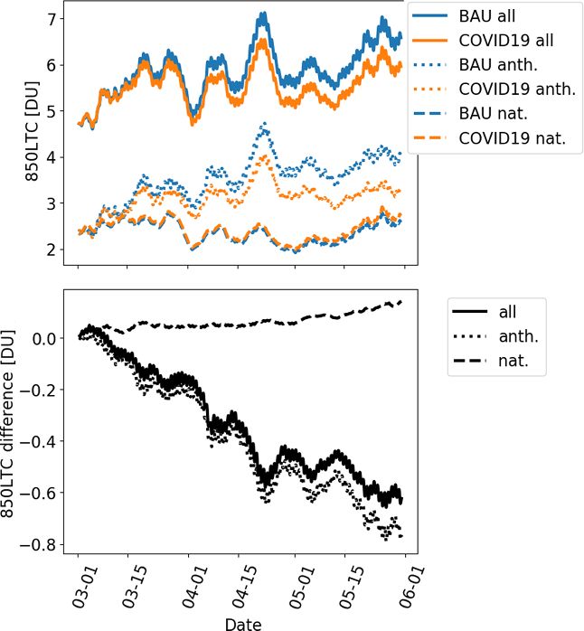
Environ. Res. Lett. 16 (2021) 064005                                                                  M Mertens et al

For our simulations we employ a regional chemistry          COSMO refinement (nest) is centred over the North
climate model (CCM) on-line nested into a global            Atlantic and covers Europe, the North Atlantic and
CCM, which is relaxed to operational meteorological         parts of North America with a resolution of approx-
analysis, to assess the impact of reduced emissions on      imately 50 km (see figure 1). The regional model is
boundary layer ozone in Europe. To complement pre-          only forced by the boundary conditions and other-
vious results based on observations, which are subject      wise evolves freely.
to changes in both, meteorology and emissions, and               Chemistry schemes for gas and aqueous phase
hence more difficult to interpret ([5, 6]) we use the       chemistry are applied consistently in the global model
CCM in a so-called quasi-chemistry transport model          and the regional refinement as described by [17]. For
(QCTM) mode to suppress feedback from chemistry             calculation of chemical kinetics, we use the MESSy
on meteorology [12]. Furthermore, our model setup           submodel Module Efficiently Calculating the Chem-
allows for an attribution of ozone to various emission      istry of the Atmosphere (MECCA [24]). The chemical
sectors (e.g. land transport, aviation, shipping) via a     mechanism includes the chemistry of ozone, meth-
tagging technique as described by [13–15].                  ane, and odd nitrogen. Alkynes and aromatics are
    This paper is structured as follows: section 2 con-     not considered, but alkenes and alkanes are con-
tains the description of the atmospheric model(s)           sidered up to C4 . The Mainz Isoprene Mechanism
and simulation set-ups along with the emission scen-        (MIM1 [25]) is applied for the chemistry of isoprene
arios and a short description of the measurement            and some non-methane hydrocarbons. Scavenging of
data employed. The results are presented in section 3.      trace gases by clouds and precipitation is calculated
Finally, we discuss our results (section 4) and state our   by the submodel SCAV (scavenging of traces gases by
conclusions (section 5).                                    clouds and precipitation [26]). Dry deposition is con-
                                                            sidered according to [27].
2. Methods                                                       To avoid feedbacks of the chemistry on dynam-
                                                            ics, the global and the regional models are oper-
2.1. Atmospheric modelling and simulation set-up            ated in the so-called QCTM mode [12]. In this
For our analyses we employ the CCM MECO(n)                  mode mixing ratios of greenhouse gases with respect
(MESSy-fied ECHAM COSMO models nested n-                    to the calculation of radiative fluxes are prescribed
times) in a modified version of MESSy 2.54 ([16, 17]).      from daily averaged values of a previous simula-
Here, we use a MECO(1) setup which nests one                tion. This previous simulation covers the same time
instance of the regional CCM COSMO-CLM/MESSy                period and uses the same set-up as the BAU sim-
[18] into the global CCM EMAC using the MESSy               ulation described below. Due to the usage of the
infrastructure ([19, 20]). COSMO–CLM is the com-            QCTM-mode the emission sensitivities described in
munity model of the German regional climate                 section 2.2 do not affect the meteorological situation.
research community jointly further developed by the         This means, that in both simulations the meteorology
CLM-Community [21]. EMAC in turn uses the gen-              (i.e. wind, temperature, humidity etc.) is identical.
eral circulation model ECHAM5 [22] as a base model.         The transport and processing of chemical constitu-
Our simulations cover the period 1 March–1 July             ents is, however, different due to the changed primary
2020.                                                       emissions.
    The global model, EMAC, was operated at a                    Anthropogenic and natural emissions are pre-
T42L90MA triangular spectral resolution, which cor-         scribed by flux conditions at the lower boundary.
responds to a quadratic Gaussian grid of approx-            In our reference or BAU simulation anthropogenic
imately 2.8◦ × 2.8◦ (roughly 300 km) and 90                 emissions are prescribed according to the EDGAR
model levels in the vertical, which extend up to the        4.3.1 emission inventory for the year 2010 [28]. From
middle atmosphere (∼0.01 hPa). Meteorological pro-          the emission sectors in EDGAR 4.3.1 we distinguish
gnostic variables, i.e. divergence, vorticity, temperat-    the emission sectors land transport (TRA), anthropo-
ure (excluding mean temperature) and (logarithm of)         genic non-traffic fossil fuel use in industry and house-
surface pressure, have been ‘nudged’ by Newtonian           holds (in the following referred to ANT emissions,
relaxation to European Centre for Medium-Range              ANT), and shipping. Emissions of agricultural waste
Weather Forecasts (ECMWF’s) operational analyses            burning, biomass burning and aviation are prescribed
data for the simulation period with 6 h temporal res-       according to the RCP 8.5 emission inventory for the
olution. The nudging coefficients are applied in a          year 2020 [29, 30].
way that the large-scale synoptic patterns follow the            Biogenic emissions of soil NOx and biogenic iso-
ECMWF data, but the model can develop its own               prene are interactively calculated by the global and
small-scale dynamics (for more details see [23]).           the regional model according to the parameterisa-
    At the nesting boundaries, the global model             tions of [31] and [32], respectively. NOx emissions
passes boundary conditions with respect to dynamics         from lightning are parameterised based on the cloud-
and chemistry to the regional model with a high tem-        top height [33] and scaled to global total emissions
poral resolution [17]. In this simulation, the regional     of ∼5 Tg(N)/a. The emissions of lightning-NOx are

                                               2
Environ. Res. Lett. 16 (2021) 064005 M Mertens et al
Table 1. Assumed emission reductions (in per cent) in the COVID19 sensitivity simulation compared to the BAU simulation. The total
emissions are given in the supplement (section S3).
Sector/Region Land transport (TRA) Anthropogenic non-traffic (ANT) Shipping (Ship) Aviation (Avia.)
Europe (EU) −50% −30%
East Asia (EA) −20% −30%
North America (NA) −20% −30%
Rest of the world (RoW) −30% −20%
Globally −20% −90%
calculated in EMAC only and mapped to the finer reductions should be seen as first-order estimates and
resolved model instance (see [17]). were chosen during the early phase of the COVID-
The source attributions method (tagging) is an 19 pandemic. Further, the qualitative conclusions (see
accounting system following the relevant reaction next sections) are not critically dependent on the
pathways and is based on the method introduced by exact emission reductions.
[34]. This diagnostic method allows to completely A reduction of 30% has been assumed for ANT
decompose the budgets of considered chemical spe- emissions (comprising industry and households) in
cies into contributions of sources. For the source Europe (EU), North America (NA) and East Asia
attribution, the source terms, e.g. emissions, of the (EA) and of 20% for the rest of the world (RoW).
considered chemical species (odd oxygen, NOy , CO, TRA emissions have been reduced by 30%, 20%
PAN, VOCs, OH and HO2 ), are fully decomposed and 20% in RoW, NA and EA, respectively, while
into N unique categories. In the present study we a higher reduction factor of 50% has been assumed
distinguish N = 16 different tagging categories (see in EU. Our estimates of emissions in Europe are
section S4 in the supplement (available online at in line with emission reduction factors for indi-
stacks.iop.org/ERL/16/064005/mmedia)). The details vidual countries in Europe estimated to be mostly
of the tagging method are described by [14] and [15] in the order of 10%–30% for industry and 30%–
and the application in MECO(n) is demonstrated 80% for road transport [37]. Shipping emissions
by [35]. The source attribution method allows us to have been reduced by 20%, and aircraft emis-
separate the contributions of natural sources (tag- sion by 90%, following ICAO movement data [38],
ging categories: stratosphere, CH4 , biogenic, N2 O, which estimate a reduction of 94% in global aircraft
biomass burning and lightning) and anthropogenic movements.
emissions (all other sources, see section S4 in the
supplement). 2.3. Measurement data
We have performed two simulations, which both As observational data (for the period 2017–2020) we
use the same meteorology: BAU (BAU, with the ref- used the air quality E1a & E2a data sets (formerly
erence emissions described above) and COVID19, known as AirBase) available at [39]. We have set neg-
which assumes emission reductions in the sectors ative concentrations or unrealistic large concentra-
land transport (TRA), ANT, shipping and aviation as tions to missing values for further analyses. In total
described in section 2.2. this corresponds to less than 0.2% of all datapoints
which are used in our analysis. As the resolution
2.2. Assumptions on emissions during first half of of our model does not account for localised effects
2020 [35], we use only data of stations which are clas-
For the COVID19 simulation we scale all emission sified as ‘background’-stations (dataflag AirQuality
sectors/species (CO, NOx , SO2 , NH3 , and VOC) con- StationType) in an area classified as either ‘remote’ or
tained in the EDGAR 4.3.1 inventory and the aviation ‘remote-rural’ (dataflag AirQualityStationArea).
NOx emissions of the RCP 8.5 emission inventory We chose the subset of stations (in total 273),
(table 1) in order to represent the reduced anthropo- which are available for the whole period for our ana-
genic activities in individual regions of the globe. The lyses (section S7 in the supplement).
reduction factors are constant over the whole simu- Similar to many comparable models (e.g. [40]),
lation period (1 March–1 July 2020). Total emissions MECO(n) has deficits in simulating the night time
are given in the supplement (section S3). ozone [35]. Usually, the simulated ozone levels during
BAU and COVID19 use the same initial con- night are too high, while the model is able to capture
ditions, but different emissions starting from 1 the ozone peak during day. Therefore, the compar-
March 2020. Current estimates of rescaled emission ison of model results and measurements is restricted
factors for early to mid-2020 show large uncertain- to the period 10–17 UTC.
ties and strong temporal variability (see figures 2–6 To compare the model results with the meas-
in [36]). Our study is highly idealized (e.g. by assum- urements, we sample the one-hourly instantaneous
ing time-independent reductions) and the assumed model output at the lowest model layer at the
3Environ. Res. Lett. 16 (2021) 064005 M Mertens et al
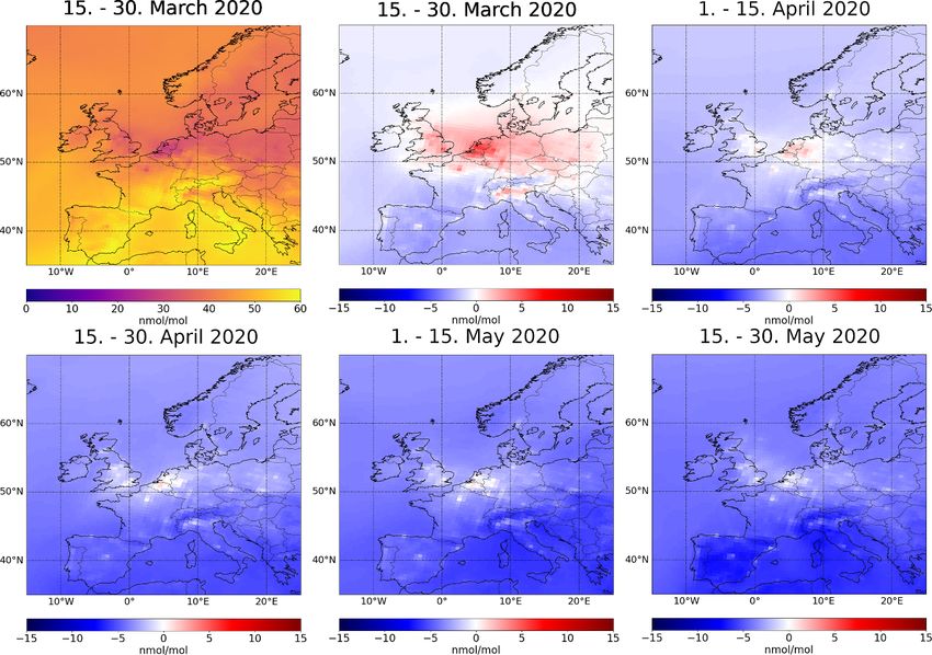
Figure 1. Ground-level ozone in nmol mol−1 over Europe for 15–30 March 2020 as simulated by BAU (upper left). Other panels
show differences of (COVID19-BAU) of ground-level ozone (in nmol mol−1 ) for the indicated periods.
positions of the respective observation stations. All masses from lower latitudes to Europe. The reduc-
datapoints, which are missing in the observational tion of anthropogenic emissions due to COVID-19
data for the year 2020, were set to missing values also continuously reduces the ozone production, resulting
for the model data. in a by 0.6 DU smaller increase of LTC by the end of
May. Due to the same dynamics of both simulations
3. Results the part of the variability driven by meteorology is
aligned.
3.1. Lower tropospheric ozone response to The ozone production efficiency (OPE), i.e. the
emission reductions net-ozone production per NOx molecule, however,
In our analyses we focus on the results of the regional increases in the COVID19 simulation compared to
model over the area 15 ◦ W–25 ◦ E to 35 ◦ N–70 ◦ N BAU (supplementary material figures S2 and S3
(as shown in figure 1), which is centred over Europe. and section S2 for the definition). In addition, the
Hence, we will refer to quantities over this domain commonly used indicator of the ozone production
as European values. Further, we focus on the period regime, the ratio of the production rate of H2 O2 to the
March–May 2020. production rate of HNO3 [41], also increases every-
The simulated near-surface ozone under BAU where (figures S4 and S5 in the supplement). This
conditions shows large temporal variability over indicates a shift of ozone production from a NOx -
Europe during the analysed period (figure 2 and saturated or intermediate to a NOx -limited regime, in
figure S1 in the supplement). The lower tropo- line with previous findings e.g. by [9].
spheric ozone column (LTC; from the surface up As a consequence, the contribution of natural
to 850 hPa) increases from around 5 DU in March emission sources to the ozone LTC increases by 0.1–
to up to ∼7 DU in May 2020 due to increased 0.2 DU (figure 2 lower panel), despite unchanged
ozone production arising from increased photochem- emissions and partly counteracts the decrease of
ical activity in the course of the year. We choose ozone of around 0.7 DU from anthropogenic sources
850 hPa as upper boundary of the LTC as this typ- (figure 2 bottom).
ically includes the planetary boundary layer every- The change in OPE (cf. figures S2 and S3 in the
where in Europe except over the alpine region. The supplement) is not uniform over Europe. Especially
peaks with large values of the ozone column espe- during 15–30 March an increase in ozone due to
cially mid of April are mainly related to events in the COVID-19 related emission reduction is simu-
which high pressure ridges transport ozone rich air lated in the area of the Benelux countries and only
4Environ. Res. Lett. 16 (2021) 064005 M Mertens et al
Figure 3. PDFs of ozone concentration at all
‘rural’/’rural-remote’ background stations for the BAU and
COVID19 simulations as well as for the measurements of
2020 and the combinations of all measurements 2017–2019
(for the period 15 March–31 May).
Figure 2. Lower tropospheric ozone columns in DU (for
pressure higher than 850 hPa) averaged over the region
shown in figure 1. (Top) Total lower tropospheric columns a shift of the modal values from 102 µg m−3 in
for the (blue) BAU and the (orange) COVID19 simulation BAU to 93 µg m−3 in COVID19. Hence, the shift
for (solid) all, (dotted) anthropogenic and (dashed) natural
sources. The latter two are diagnosed by the source towards lower values is similar to that of the meas-
apportionment method. (Bottom) Differences of the LTCs urements between 2017 to 2019 and 2020, but the
(COVID19-BAU) with line styles as in the top panel. magnitude is overestimated. Considering only ozone
values around noon or around afternoon yields sim-
ilar results (see figures S7 and S8 in the supplement).
after roughly a month this increased ozone vanishes Also, the comparison of the difference between the
and lower ozone mixing ratios compared to the BAU daily ozone minimum and the daily ozone max-
simulation dominate over Europe in the COVID19 imum showed similar biases (see figure S9 in the
simulation (figure 1). Large reductions of ozone are supplement). In general, however, the difference
found in Southern Europe, except for the polluted between the BAU and COVID19 simulation shows
metropolitan areas (e.g. around Madrid, Barcelona the same tendency as the difference between
and Rome) and areas like the Po-valley. In these the measurements from 2020 and 2017–2019,
regions the OPE is rather low and favours an increase respectively.
in ozone productivity with reduced emissions, coun- Of course, the difference between the measure-
teracting the ozone production decrease from the ments of 2017–2019 and 2020 is also influenced
reduction in precursor emissions. Averaged over the by the meteorological conditions, while the differ-
period 15 March–31 May the decrease of surface ences between our BAU and COVID19 simulations
NOx was between −10% and −40% over the differ- is caused by the emission reductions only. Neverthe-
ent regions in Europe. At the same time, the reduc- less, the comparison of the measurement data indic-
tions of ozone were only up to about −8% at max- ates that a reduction of ground-level ozone due to the
imum, while especially in Mid Europe ground-level emission changes under COVID-19 conditions is very
ozone increased by up to 15% (see figure S6 in the likely. This allows us to continue with our analysis of
supplement). changes with respect to ozone sources related to the
Our findings of lower ozone values in rural reduced emissions.
areas are largely supported by surface measurements
(figure 3): The daytime measured ozone concen- 3.2. Attributing ozone reductions to emissions
trations in rural areas have modal values of 89 and sectors
84 µg m−3 in the pre-COVID-19 years (2017–2019) During May (1 May–30 May) the mean ozone LTC
and during the COVID-19 pandemic (2020), respect- over the European domain (as depicted in figure 1)
ively for spring (15 March–31 May), i.e. the probab- is roughly 6.1 and 5.6 DU for BAU and COVID19,
ility density functions are shifted towards lower val- respectively (see figure 2). The ozone decline in
ues (additional values are given in section S6 in the the COVID19 simulation stems from the reduc-
supplement). Here, we use the period 2017–2019 as tion in anthropogenic emissions, which overcom-
an indicator of what might have happened without pensates the enhanced ozone productivity. This is
COVID-19, i.e. for comparison with the BAU sim- caused by the reduction of ozone precursor emis-
ulation. Even though the model generally simulates sions (mainly NOx and VOCs) and the corres-
larger mean ozone concentrations, the results show ponding ozone increase related to natural sources,
5Environ. Res. Lett. 16 (2021) 064005 M Mertens et al
Figure 4. Contributions to lower tropospheric ozone columns (in percent) in the BAU (blue), COVID19 (orange) simulation and
their differences (red, in percentage-points) during May 2020. Avia. is aviation and ship is shipping. Other natural sources include
emissions from lightning, soils, biomass burning and methane depletion. Categories marked with two asterisks refer to the
vertical axis on the right, all others to the vertical axis on the left.
such as soil emissions, biomass burning, lightning (e.g. [43, 44]). This can be seen by the increased
and methane depletion (figure 4). The absolute contribution of stratospheric ozone to the LTC of
value of mean LTC from natural (anthropogenic) ozone from 6.5% to 7.3% (figure 4). As stratospheric
sources increases (decreases) from approximately 2.3 ozone is unperturbed in our COVID19 simulation
(3.8) DU to roughly 2.4 (3.2) DU from BAU to the influx to the troposphere is almost unchanged.
COVID19. This translates to relative contributions Therefore, the increase of the contribution of ozone
of natural emissions to the mean LTC over Europe from the stratosphere indicates an increase of the
of roughly 37% and 43% in BAU and COVID19, tropospheric ozone lifetime. The absolute contri-
respectively. bution of stratospheric ozone to the LTC increases
The relative contributions of almost all anthropo- by around 2%, indicating an increase of the ozone
genic emissions sectors to the LTC decrease (figure 4). lifetime of 2%.
The sectors with the largest contribution decrease
to LTC ozone are the aviation sector (90% emis- 4. Discussion
sion reduction) with a decrease of 2.7% points and
the TRA sector in Europe (50% emission reduction) By design our study is highly idealized as we assume
with a decrease of 1.6% points. This corresponds to that the emission reductions take place world-wide at
an overall decrease of the contribution of anthropo- the same time and without temporal variability from
genic emissions from roughly 63% to 57%. The rel- March to June. There are first studies, which present
ative contribution of the emission sectors TRA NA more detailed emission modelling for Europe and
and shipping increase slightly, but their absolute con- Asia (e.g. [36, 37, 45, 46]). Generally, our assumed
tributions (section S5 in the supplement) decrease reductions are in line with [36] however our estim-
indicating that the ozone productivity of these two ates for EA ANT and shipping are slightly larger,
sectors increases slightly more than in the other emis- whereas NA TRA reductions are somewhat low. How-
sion sectors and regions. ever, the estimates presented in [36] show consider-
Further, our results indicate that European emis- able uncertainties. Our results need to be interpreted
sions (i.e. TRA EU + ANT EU) contribute only while keeping these simplifications in mind.
around 15% (BAU) and 13% (COVID19) to lower Compared to, e.g. [45, 47], our study analyses for
tropospheric ozone in Europe during May 2020. All the first time the impact of the emission reduction
other anthropogenic emissions (i.e. shipping, avi- on ozone using a source apportionment method. This
ation, non-EU TRA and non-EU ANT) contrib- method allows a more detailed understanding of the
ute roughly 48% (BAU) and 44% (COVID19). This changes of the ozone chemistry and is able to attrib-
clearly indicates the well-known importance of long- ute the changes to certain emission sectors. Therefore,
range transport for ozone pollution (e.g. [42]). In our study delivers important additional insights.
addition, the change of the chemical regime implies Even though our emission reductions in Europe
an increase of the ozone lifetime, since a reduction of −50% and −30% of LT and ANT, respect-
of ozone leads to a reduction of OH and therefore ively, are very large, we see only a rather small
HOx related ozone depletion rates in the troposphere decrease of mean lower tropospheric ozone columns
6Environ. Res. Lett. 16 (2021) 064005 M Mertens et al
of around 8% during May 2020 over Europe (see tropospheric ozone in a period of reduced anthropo-
figure 2). The main reason for this is the increas- genic emissions as during the recent COVID-19 pan-
ing OPE per NOx molecule (see definition of the demic compared to an emission scenario without the
OPE in the supplement). This leads to a small impact of the COVID-19 pandemic (BAU). Our sim-
increase (∼0.1 DU) in the ozone values produced ulations with a coupled global and regional CCM and
from natural emissions (figures 2 and 3). With a source attribution technique show:
respect to potential mitigation options this result
demonstrates that detailed assessments are needed • the ozone LTC averaged over the European domain
to judge, whether planned emissions reductions are in the COVID19 simulation become continuously
sufficient to decrease tropospheric ozone burdens lower over time for around three months compared
substantially. Indeed, some modelling studies (e.g. to the BAU simulation before a new equilibrium is
[45, 47]) indicate a similarly low response of ozone. reached.
Some measurement studies (e.g. [4, 6, 48–50]) • there are large spatial inhomogeneities with respect
even found an increase of ozone near city centres to this overall trend in ozone LTCs, which are
during March 2020 compared to previous years, related to the ozone production regimes.
probably due to decreased NOx emissions. How- • the overall shift towards smaller ozone LTCs in
ever, also the role of meteorology needs to be COVID19 and BAU is also found in measurement
considered [51]. data from ground-based stations.
Our study further highlights that due to the rather • changes in anthropogenic emissions cause the
long lifetime of ozone, the emissions in other parts of changes in ozone LTCs and are to some degree com-
the world strongly influence European ozone levels. pensated by enhanced ozone productivity from
Therefore, reducing emissions only in Europe will natural sources. Due to the increase of the OPE
most likely not lead to envisaged ozone decreases in the reductions in ozone are much smaller than the
Europe. emission reductions. In our case NOx at ground-
Our simulation results show that around three level is reduced by up to 40% in Europe, while
months are needed until the difference of the ozone ground-level ozone changes are in the range of
LTC between BAU and COVID19 (see figures 2 and −8% to +15% for Europe.
S1) equilibrates. In most countries the strong emis-
sion reductions took place for some weeks, only (e.g. The results of our study are not only relevant
[37]). Therefore, the actual effect of the emission for ozone changes related to the recent reduction
reductions during COVID-19 in spring 2020 is likely in emissions due to the COVID19 pandemic, they
to be much smaller than the maximum signal of our also are a starting point for discussing mitigation
idealized study. strategies. In line with our model results, measure-
Due to the uncertainty of the applied emission ments during the first half of 2020 and first modelling
inventory for BAU and the non-linearity of the ozone studies show ozone responses which are much smal-
production (e.g. 13) our simulated response of the ler than the emission reductions. This indicates that
emission reduction (figure 2) might still be overes- strong emission reductions are needed world-wide
timated, if our BAU emissions are underestimated. to achieve substantially reduced tropospheric ozone
Indeed, the shift of ozone values between our BAU levels.
and COVID19 simulation is larger as the shift in
the measurements from 2017 to 2019 and 2020. This
Data availability statement
could indicate an overestimated response, but this dif-
ference could also be caused by differences of the met-
The data that support the findings of this study are
eorological conditions in the previous years (2017–
available upon reasonable request from the authors.
2019) compared to 2020.
The main focus of our study is on near ground-
level ozone, focusing mainly on-air quality related Acknowledgments
issues. Besides this, changes in ozone and other emis-
sions influence also the climate. However, as already We thank Astrid Kerkweg, FZ Jülich, for her ongo-
been shown by [3], the overall climate impact of ing support and the MECO(n) developments and
the strong emission reductions during COVID-19 is Christoph Kiemle, DLR, for very helpful com-
small. According to [3], the decrease of ozone pre- ments improving the quality of the manuscript.
cursors leads to a short-term cooling, which is offset Further, we thank the MESSy consortium and the
by a warming effect due to less aerosol. CLM-Community for their model developments
and ongoing support. The work described in this
5. Conclusion paper received funding from the DLR projects
TraK (Transport und Klima) and Eco2Fly and by
We conducted a sensitivity experiment (COVID19) to the Initiative and Networking Fund of the Helm-
analyse the processes occurring with respect to lower holtz Association through the project ‘Advanced
7Environ. Res. Lett. 16 (2021) 064005 M Mertens et al
Earth System Modelling Capacity’ (ESM). Indi- [13] Grewe V, Tsati E and Hoor P 2010 On the attribution of
vidual authors receive funding from the European contributions of atmospheric trace gases to emissions in
atmospheric model applications Geosci. Model Dev.
Union’s Horizon 2020 research and innovation pro-
3 487–99
gramme under Grant Agreement No. 875036 within [14] Grewe V, Tsati E, Mertens M, Frömming C and Jöckel P 2017
the Aeronautics project ACACIA. We thank the Contribution of emissions to concentrations: the TAGGING
ECWMF for providing operational meteorological 1.0 submodel based on the modular earth submodel system
(MESSy 2.52) Geosci. Model Dev. 10 2615–33
analysis. This work used resources of the Deutsches
[15] Rieger V S, Mertens M and Grewe V 2018 An advanced
Klimarechenzentrum (DKRZ) granted by its Sci- method of contributing emissions to short-lived chemical
entific Steering Committee (WLA) under project species (OH and HO2): the TAGGING 1.1 submodel based
ID bd0617. on the modular earth submodel system (MESSy 2.53) Geosci.
Model Dev. 11 2049–66
[16] Kerkweg A and Jöckel P 2012 The 1-way on-line coupled
ORCID iDs atmospheric chemistry model system MECO(n)—part 1:
description of the limited-area atmospheric chemistry model
Mariano Mertens https://orcid.org/0000-0003- COSMO/MESSy Geosci. Model Dev. 5 87–110
3549-6889 [17] Mertens M, Kerkweg A, Jöckel P, Tost H and Hofmann C
2016 The 1-way on-line coupled model system
Patrick Jöckel https://orcid.org/0000-0002-8964- MECO(n)—part 4: chemical evaluation (based on MESSy
1394 v2.52) Geosci. Model Dev. 9 3545–67
Sigrun Matthes https://orcid.org/0000-0002- [18] Kerkweg A and Jöckel P 2012 The 1-way on-line coupled
5114-2418 atmospheric chemistry model system MECO(n)—part 2:
on-line coupling with the multi-model-driver, (MMD)
Volker Grewe https://orcid.org/0000-0002-8012- Geosci. Model Dev. 5 111–28
6783 [19] Jöckel P, Kerkweg A, Pozzer A, Sander R, Tost H, Riede H,
Robert Sausen https://orcid.org/0000-0002-9572- Baumgaertner A, Gromov S and Kern B 2010 Development
2393 cycle 2 of the modular earth submodel system (MESSy2)
Geosci. Model Dev. 3 717–52
[20] Jöckel P et al 2016 Earth system chemistry integrated
References modelling (ESCiMo) with the modular earth submodel
system (MESSy) version 2.51 Geosci. Model Dev. 9 1153–200
[1] Diffenbaugh N S et al 2020 The COVID-19 lockdowns: a [21] Rockel B, Will A and Hense A 2008 The regional climate
window into the earth system Nat. Rev. Earth Environ. model COSMO-CLM (CCLM) Meteorol. Z. 17 347–8
1 470–81 [22] Roeckner E, Brokopf R, Esch M, Giorgetta M, Hagemann S,
[2] Le Quéré C et al 2020 Temporary reduction in daily global Kornblueh L, Manzini E, Schlese U and Schulzweida U 2006
CO2 emissions during the COVID-19 forced confinement Sensitivity of simulated climate to horizontal and vertical
Nat. Clim. Change 10 647–53 resolution in the ECHAM5 atmosphere model J. Clim.
[3] Forster P M et al 2020 Current and future global climate 19 3771–91
impacts resulting from COVID-19 Nat. Clim. Change [23] Jöckel P et al 2006 The atmospheric chemistry general
10 913–9 circulation model ECHAM5/MESSy1: consistent simulation
[4] Shi X and Brasseur G P 2020 The response in air quality to of ozone from the surface to the mesosphere Atmos. Chem.
the reduction of Chinese economic activities during the Phys. 6 5067–104
COVID-19 outbreak Geophys. Res. Lett. 47 e2020GL088070 [24] Sander R et al 2019 The community atmospheric chemistry
[5] Bauwens M et al 2020 Impact of coronavirus outbreak on box model CAABA/MECCA-4.0 Geosci. Model Dev.
NO2 pollution assessed using TROPOMI and OMI 12 1365–85
observations Geophys. Res. Lett. 47 e2020GL087978 [25] Pöschl U, Von Kuhlmann R, Poisson N and Crutzen P 2000
[6] Keller C A et al 2021 Global impact of COVID-19 Development and intercomparison of condensed isoprene
restrictions on the surface concentrations of nitrogen oxidation mechanisms for global atmospheric modeling J.
dioxide and ozone Atmos. Chem. Phys. 21 3555–92 Atmos. Chem. 37 29–52
[7] Dodge M 1977 Combined use of modeling techniques and [26] Tost H, Jöckel P, Kerkweg A, Sander R and Lelieveld J 2006
smog chamber data to derive ozone precursor relationships Technical note: a new comprehensive SCAVenging submodel
Int. Conf. on Photochemical Oxidant Pollution and Its Control: for global atmospheric chemistry modelling Atmos. Chem.
Proc. vol II, ed B Dimitriades (Research Triangle Park, NC: Phys. 6 565–74
U.S. Environmental Protection Agency, Environmental [27] Kerkweg A, Buchholz J, Ganzeveld L, Pozzer A, Tost H and
Sciences Research Laboratory) pp 881–9 EPA/600/3-77-001b Jöckel P 2006 Technical note: an implementation of the dry
[8] Lin X, Trainer M and Liu S C 1988 On the nonlinearity of removal processes DRY DEPosition and SEDImentation in
the tropospheric ozone production J. Geophys. Res. the modular earth submodel system (MESSy) Atmos. Chem.
93 15879–88 Phys. 6 4617–32
[9] Grewe V, Dahlmann K, Matthes S and Steinbrecht W 2012 [28] Crippa M, Janssens-Maenhout G, Dentener F, Guizzardi D,
Attributing ozone to NOx emissions: implications for Sindelarova K, Muntean M, Van Dingenen R and Granier C
climate mitigation measures Atmos. Environ. 59 102–7 2016 Forty years of improvements in European air quality:
[10] Gislason S R et al 2011 Characterization of Eyjafjallajökull regional policy-industry interactions with global impacts
volcanic ash particles and a protocol for rapid risk Atmos. Chem. Phys. 16 3825–41
assessment Proc. Natl Acad. Sci. 108 7307–12 [29] van Vuuren D P et al 2011 The representative concentration
[11] Turnbull K, Johnson B, Marenco F, Haywood J, Minikin A, pathways: an overview Clim. Change 109 5–31
Weinzierl B, Schlager H, Schumann U, Leadbetter S and [30] Riahi K, Rao S, Krey V, Cho C, Chirkov V, Fischer G,
Woolley A 2012 A case study of observations of volcanic ash Kindermann G, Nakicenovic N and Rafaj P 2011 RCP 8.5—a
from the Eyjafjallajökull eruption: 1. In situ airborne scenario of comparatively high greenhouse gas emissions
observations J. Geophys. Res. 117 D00U12 Clim. Change 109 33–57
[12] Deckert R, Jöckel P, Grewe V, Gottschaldt K-D and Hoor P [31] Yienger J J and Levy H 1995 Empirical model of global
2011 A quasi chemistry-transport model mode for EMAC soil-biogenic NOx emissions J. Geophys. Res. Atmos. 100
Geosci. Model Dev. 4 195–206 11447– 64
8Environ. Res. Lett. 16 (2021) 064005 M Mertens et al
[32] Guenther A et al 1995 A global model of natural volatile [43] Stevenson D S et al 2006 Multimodel ensemble simulations
organic compound emissions J. Geophys. Res. 100 8873–92 of present-day and near-future tropospheric ozone J.
[33] Price C, Rind D 1992 A simple lightning parameterization Geophys. Res. 111 D08301
for calculating global lightning distributions J. Geophys. Res. [44] Grewe V 2007 Impact of climate variability on tropos pheric
97 9919–33 ozone Science of The Total Environment. 374 167–81
[34] Grewe V 2013 A generalized tagging method Geosci. Model [45] Menut L, Bessagnet B, Siour G, Mailler S, Pennel R and
Dev. 6 247–53 Cholakian A 2020 Impact of lockdown measures to combat
[35] Mertens M, Kerkweg A, Grewe V, Jöckel P and Sausen R 2020 Covid-19 on air quality over Western Europe Sci. Total
Are contributions of emissions to ozone a matter of Environ. 741 140426
scale?—a study using MECO(n) (MESSy v2.50) Geosci. [46] Xing J, Li S, Jiang Y, Wang S, Ding D, Dong Z, Zhu Y and
Model Dev. 13 363–83 Hao J 2020 Quantifying the emission changes and associated
[36] Doumbia T et al 2021 Changes in global air pollutant air quality impacts during the COVID-19 pandemic on the
emissions during the COVID-19 pandemic: a dataset for North China Plain: a response modeling study Atmos. Chem.
atmospheric chemistry modeling Earth Syst. Sci. Data Phys. 20 14347–59
Discuss. (https://doi.org/10.5194/essd-2020-348) [47] Dentener F, Emberson L, Galmarini S, Cappelli G,
[37] Guevara M et al 2021 Time-resolved emission reductions for Irimescu A, Mihailescu D, Van Dingenen R and
atmospheric chemistry modelling in Europe during the Van Den Berg M 2020 Lower air pollution during
COVID-19 lockdowns Atmos. Chem. Phys. 21 773–97 COVID-19 lock-down: improving models and methods
[38] ICAO (International Civil Aviation Organisation) 2020 estimating ozone impacts on crops Phil. Trans. R. Soc. A
Effects of novel coronavirus (COVID-19) on civil aviation: 378 20200188
economic impact analysis ICAO 8 May 2020 (Montréal: Air [48] Lee J D, Drysdale W S, Finch D P, Wilde S E and Palmer P I
Transportation bureau) 2020 UK surface NO2 levels dropped by 42 % during the
[39] European Air Quality Portal E1a & E2a data sets (available COVID-19 lockdown: impact on surface O3 Atmos. Chem.
at: https://discomap.eea.europa.eu/map/fme/ Phys. 20 15743–59
AirQualityExport.htm) (Accessed 8 January 2021) [49] Sicard P, De Marco A, Agathokleous E, Feng Z, Xu X,
[40] Travis K R and Jacob D J 2019 Systematic bias in evaluating Paoletti E, Rodriguez J J D and Calatayud V 2020 Amplified
chemical transport models with maximum daily 8 h average ozone pollution in cities during the COVID-19 lockdown
(MDA8) surface ozone for air quality applications: a case Sci. Total Environ. 735 139542
study with GEOS-Chem v9.02 Geosci. Model Dev. 12 3641–8 [50] Salma I, Vörösmarty M, Gyöngyösi A Z, Thén W and
[41] Sillman S 1995 The use of NOy , H2 O2 , and HNO3 Weidinger T 2020 What can we learn about urban air quality
as indicators for ozone-NOx -hydrocarbon with regard to the first outbreak of the COVID-19
sensitivity in urban locations J. Geophys. Res. pandemic? A case study from central Europe Atmos. Chem.
100 14175–88 Phys. 20 15725–42
[42] Monks P S et al 2015 Tropospheric ozone and its precursors [51] Petetin H, Bowdalo D, Soret A, Guevara M, Jorba O,
from the urban to the global scale from air quality to Serradell K and Pérez García-Pando C 2020 Meteorology-
short-lived climate forcer Atmos. Chem. Phys. normalized impact of the COVID-19 lockdown upon NO2
15 8889–973 pollution in Spain Atmos. Chem. Phys. 20 11119–41
9You can also read