Increasing Robustness in the Detection of Freezing of Gait in Parkinson's Disease - MDPI
←
→
Page content transcription
If your browser does not render page correctly, please read the page content below
Article

Increasing Robustness in the Detection of Freezing of
Gait in Parkinson’s Disease
Rubén San-Segundo 1,*, Honorio Navarro-Hellín 2, Roque Torres-Sánchez 3, Jessica Hodgins 2
and Fernando De la Torre 2
 1 Information Processing and Telecommunications Center, E.T.S.I. Telecomunicación. Universidad
   Politécnica de Madrid, Madrid, Spain; ruben.sansegundo@upm.es
 2 Robotics Institute, Carnegie Mellon University, Spain; hono.navarro@gmail.com (H.N.-H);

   jkh@cs.cmu.edu (J.H.); ftorre@cs.cmu.edu (F.D.l.T.)
 3 Dpto de Ingeniería de Sistemas y Automática, Escuela Técnica Superior de Ingeniería Industrial,

   Universidad Politécnica de Cartagena, Spain; roque.torres@upct.es
 * Correspondence: ruben.sansegundo@upm.es; Tel.: +34- 910672225

 Received: 19 December 2018; Accepted: 18 January 2019; Published: 22 January 2019

 Abstract: This paper focuses on detecting freezing of gait in Parkinson’s patients using body-worn
 accelerometers. In this study, we analyzed the robustness of four feature sets, two of which are new
 features adapted from speech processing: mel frequency cepstral coefficients and quality
 assessment metrics. For classification based on these features, we compared random forest,
 multilayer perceptron, hidden Markov models, and deep neural networks. These algorithms were
 evaluated using a leave-one-subject-out (LOSO) cross validation to match the situation where a
 system is being constructed for patients for whom there is no training data. This evaluation was
 performed using the Daphnet dataset, which includes recordings from ten patients using three
 accelerometers situated on the ankle, knee, and lower back. We obtained a reduction from 17.3% to
 12.5% of the equal error rate compared to the previous best results using this dataset and LOSO
 testing. For high levels of sensitivity (such as 0.95), the specificity increased from 0.63 to 0.75. The
 biggest improvement across all of the feature sets and algorithms tested in this study was obtained
 by integrating information from longer periods of time in a deep neural network with
 convolutional layers.

 Keywords: Parkinson’s disease; freezing of gait; mel frequency cepstral coefficients; MFCCs; robust
 detection; deep learning; convolutional neural networks; CNNs; consecutive windows

1. Introduction
      The population structure in Europe will change significantly over the next 40 years, with the
elderly (defined as people over 65 years of age) increasing to 30% of the population by 2060 [1]. The
growth of this population will introduce new demands for managing quality of life and promoting
independence. Home care monitoring offers the potential for continuous health and well-being
supervision at home. This supervision is particularly important for people who are frail or have
chronic diseases such as Parkinson’s disease (PD). When falls occur, such a system can alert a nurse,
family member, or security staff [2]. Several monitoring systems have been presented for the
detection of falls or motion disorders in PD patients using on-body accelerometers [3,4]. Many of the
falls in PD patients are caused by a locomotion and postural disorder called freezing of gait (FOG)
[5]. FOG is a frequent PD symptom that affects almost 50% of Parkinson’s patients, and it is defined
as a “brief, episodic absence or marked reduction of forward progression of the feet despite the
intention to walk” [6]. This problem can last from a few seconds to a minute [7]. FOG events appear
more often during turns, with gait initiation, and in stressful situations. A successful intervention for
Electronics 2019, 8, 119; doi:10.3390/electronics8020119                     www.mdpi.com/journal/electronics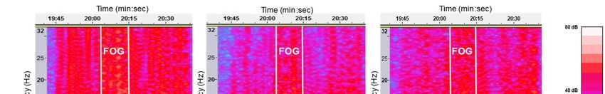
Electronics 2019, 8, 119                                                                         2 of 15

reducing the duration and frequency of FOG episodes is to induce external cues, such as a rhythmic
acoustic beat. The cueing system provides real-time auditory stimuli, helping the patient to maintain
speed and amplitude of movements when walking. These cueing systems are more effective when
applied only during FOG episodes [8,9] and, therefore, a system for reliably detecting FOG events is
required.
      The accurate supervision of patients is also important for monitoring the progression of PD. PD
patients need to visit a physician every few months to monitor the illness progression. During their
visit, the physician evaluates each patient by asking them to perform a set of activities specified in
the Movement-Disorder-Society-sponsored revision of the Unified Parkinson’s Disease Rating Scale
(MDS-UPDRS) [10]. The information gathered by the doctor is subjective because it is limited to a
short session every few months, so the physician evaluation can be influenced by the patient’s mood
that day [11] or nontypical patient behavior during the session [12]. Automatic tools for
continuously supervising PD symptoms during daily activities would provide objective long-term
data to improve the physician’s assessment. One of the symptoms that must be monitored to assess
disease progression is FOG.
      This paper describes some advances in using body-worn accelerometers to detect FOG in
Parkinson’s patients. We compared different feature sets and machine learning (ML) algorithms
using a leave-one-subject-out (LOSO) cross validation. This type of evaluation is necessary to assess
the robustness of these algorithms when monitoring patients whose data are not present in the
training set. We evaluated two feature sets already applied to FOG detection and two new feature
sets adapted from speech processing: mel frequency cepstral coefficients (MFCCs) and speech
quality assessment (SQA) metrics. We analyzed four ML algorithms: random forest, multilayer
perceptron, hidden Markov models (HMMs), and deep neural networks with convolutional layers.
This study was performed using the Daphnet dataset [13], which includes recordings from ten
patients. Our best result shows a reduction from 17.3% to 12.5% of the equal error rate, relative to the
best reported results on this dataset with a LOSO evaluation.

2. Related Work
     In this section, we review related work in body-worn sensors for monitoring Parkinson’s
patients. We also survey previous studies where several feature sets and classification algorithms
were proposed and compared for FOG detection. We pay special attention to previous studies that
used the Daphnet dataset.
     Previous studies have placed ultrathin force-sensitive switches inside the subject’s shoes [14] or
used vertical ground reaction force sensors [15] or multiaxis accelerometers [16]. Accelerometers
located on the patient’s body have been widely used to detect FOG [7,13,17,18]. The recent
widespread availability of wearable devices (fit bands, smartwatches, and smartphones) equipped
with accelerometers has facilitated this approach. The Daphnet dataset has also played a key role in
this development. Daphnet is a public dataset that includes inertial signals from ten patients
registered through three accelerometer sensors situated on the ankle, knee, and lower back. Several
papers have been published using this dataset [13,17–19].
     The detection of FOG requires the application of specific signal processing and classification
methods adapted to this type of phenomenon. Initial efforts were focused on extracting good
features [13,17,20]. Moore et al. [20] found that frequency components of leg movements in the 3–8
Hz band during FOG episodes are characteristic of this symptom and do not appear during normal
walking. They introduced a freeze index (FI) to objectively identify FOG. This FI is defined as the
power in the “freeze” band (3–8 Hz) divided by the power in the “locomotor” band (0.5–3 Hz). FOG
episodes were detected using an FI threshold, and this feature was used in later experiments [13,18].
Assam and Seidl [21] presented a study of wavelet features with different windows lengths, and
Hammerla et al. [17] proposed the empirical cumulative distribution function as feature
representation. Mazilu et al. [18] described a detailed analysis of different features using the
Daphnet dataset. The first set included FOG-oriented features such as the freezing index and the
sum of energy in the freezing (3–8 Hz) and locomotor (0.5–3 Hz) frequency bands. The second set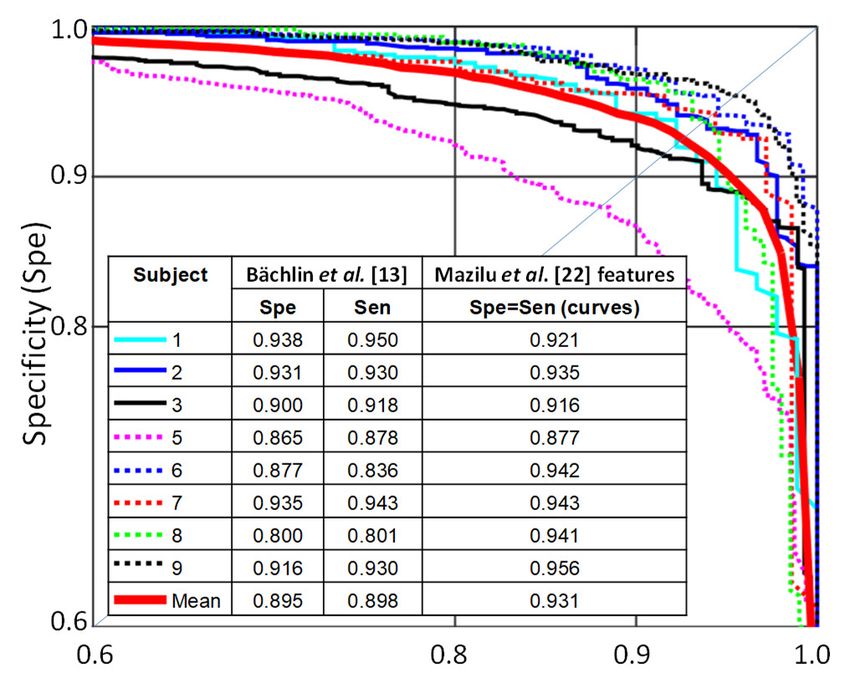
Electronics 2019, 8, 119                                                                        3 of 15

contained some features often used in activity recognition: 18 features extracted from each of the
three accelerometer axes (x, y, and z) and 6 features using data from all three axes. The best features
in the second set were the signal variance, range, root mean square, and eigenvalues of dominant
directions in the three accelerometer axes. However, the performance of these features was lower
than using FOG-specific features. Mazilu et al. also evaluated principal component analysis (PCA)
applied to the raw accelerometer signal for obtaining unsupervised features. In this paper, the
authors reported a pre-FOG status where some freezing characteristics became apparent a few
seconds before the FOG occurs.
     In another paper [22], Mazilu et al. selected the best features for FOG detection: mean, standard
deviation, variance, entropy, energy, freeze index, and power in freeze and locomotion bands. They
evaluated different algorithms: random trees, random forest, decision trees and pruned decision
trees (C4.5), naive Bayes, Bayes nets, k-nearest neighbor with one and two neighbors, multilayer
perceptron (MLP), boosting (AdaBoost), and bagging with pruned C4.5. The best performance was
obtained with AdaBoost (with pruned C4.5 as a base classifier) and random forest classifiers. All the
ensemble methods (boosting, bagging, random forests) obtained better results than the single
classifiers, with the boosting classifiers obtaining slightly better performance than the bagging
classifiers. In this evaluation, the authors used a random 10-fold cross validation (R10Fold) for each
patient, including data from the same patient in training and testing. The authors also reported an
isolated result using LOSO evaluation. This result is our baseline using the same dataset and LOSO
evaluation. We compare our results to it in section 4.2.
     In the literature, there are also papers proposing conditional random fields [21] and deep
learning algorithms for FOG detection. Ravi et al. [23] used a convolutional neural network (CNN)
with one convolutional layer for feature extraction and one fully connected layer for classification.
They obtained a specificity and a sensitivity of 0.967 and 0.719, respectively, for their R10Fold
experiments. Alsheikh et al. [19] used a deep neural network with five fully connected layers
obtaining a specificity and sensitivity of 0.915 in a R10Fold validation. The weights of the fully
connected layers were initialized using the weights of a previously trained autoencoder.
     In most of these experiments, the authors used a random 10-fold cross validation including data
from the same patient in training and testing. Our paper addresses this flaw in the analysis by using
a LOSO cross validation. LOSO evaluation is required to develop a robust FOG detection system
that can handle new patients.

3. Methods
     In this section, we detail the dataset, the signal preprocessing step, and the algorithms for
feature extraction and FOG detection. For feature extraction, we used four feature sets. The first was
the set proposed by Mazilu et al [22]. The second consisted of features used in human activity
recognition (HAR). The third set was composed of MFCCs, and the fourth included features derived
from the SQA literature, such as harmonicity, predictability, and spectral flux. For classification
algorithms, we compared random forest, multilayer perceptron, hidden Markov models, and deep
neural networks with convolutional layers.

3.1. Gait Dataset
     We used the Daphnet dataset [13] in our experiments. This public dataset contains recordings
from ten PD subjects (7 males, 66.5 ± 4.8 years) diagnosed with PD showing large variability in their
motor performance. Some participants maintained regular gait during nonfreezing episodes, while
others had a slow and unstable gait. The recordings include 3D accelerations (x, y, and z axes)
obtained from three sensors located on the ankle, thigh, and trunk (lower back) for a total of nine
inertial signals.
     The data were collected more than 12 h after the participants had taken their medication to
ensure that treatment did not prevent FOG symptoms from being observed. Participants 2 and 8
reported frequent FOG episodes with medication, so they were not asked to skip any medication
intake. The protocol consisted of several sessions, including three walking tasks performed in a
Electronics 2019, 8, 119 4 of 15
laboratory: (1) Walking back and forth in a straight line, including several 180° turns. (2) Random
walking, including a series of starts and stops and several 360° turns. (3) Walking simulating
activities of daily living (ADL), such as entering and leaving rooms or carrying a glass of water while
walking.
All sessions were recorded on a digital video camera. The ground truth labels were generated
by a physiotherapist using the video recordings. The beginning of a FOG event was specified when
the gait pattern disappeared, and the end of FOG was defined as the point in time at which the
pattern was resumed. A total of 237 FOG episodes were recorded with durations between 0.5 and
40.5 s (time while the subject was blocked and could not walk). Two subjects in the dataset (4 and
10), did not have FOG. These subjects were excluded from all experiments except for the results in
Section 4.1, where all subjects were considered for a better comparison with the results in the
literature.
3.2. Preprocessing
The raw accelerometer signals were recorded with a sampling rate of 64 Hz. This sampling rate
was adequate because the information for FOG event detection is below 20 Hz [20]. To remove the
influence of gravity, we filtered the data with a high-pass third-order Butterworth filter at 0.3 Hz.
The sample sequence was divided into a sequence of 4-s windows (256 samples) with 3-s overlap
and 1-s advance. A window was labeled as a FOG window if more than 50% of its samples were
labeled as FOG.
3.3. Feature Extraction
The main characteristic of FOG is the power increment in the frequency band of 3–8 Hz that
does not appear during normal walking [20]. When patients wanted to walk and they could not
because of freezing, a vibration often appeared in all sensors (Figure 1).
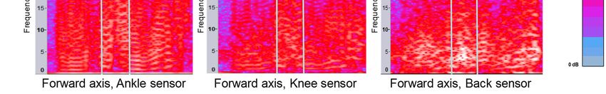
Figure 1. Spectrogram for three accelerometer signals: forward axis of ankle, knee, and back sensors.
The log energy at different frequencies is coded with blue for low energy and red for higher energy,
ranging from 0 to 80 dB. During a FOG episode, the power increases in the frequency band of 3–8 Hz.
Table 1 summarizes the four features sets considered in this study. The first set of features
contained the seven features per signal used in Mazilu et al. [22]. With nine signals, we obtained a 7 ×
9 feature vector for each 4-s window. The second set of features was composed of 90 features per
signal (90 × 9 signals) that have often been used in HAR [24]. This set included metrics obtained from
the accelerometer signals in the time and frequency domains. The third set of features consisted of
MFCCs adapted to inertial signals [25]: 12 coefficients were considered from every inertial signal (12
× 9 signals).
The fourth set consisted of three metrics adapted from the SQA field [26]. Many of these metrics
are based on the speech signal periodicity presented during vowel pronunciation. When a person
walks naturally, the accelerometer signal has high levels of periodicity and harmonicity and this
structure is broken during a FOG event. The first quality metric used was harmonicity. This metric
was computed as the autocorrelation of every window in time and frequency domains, generating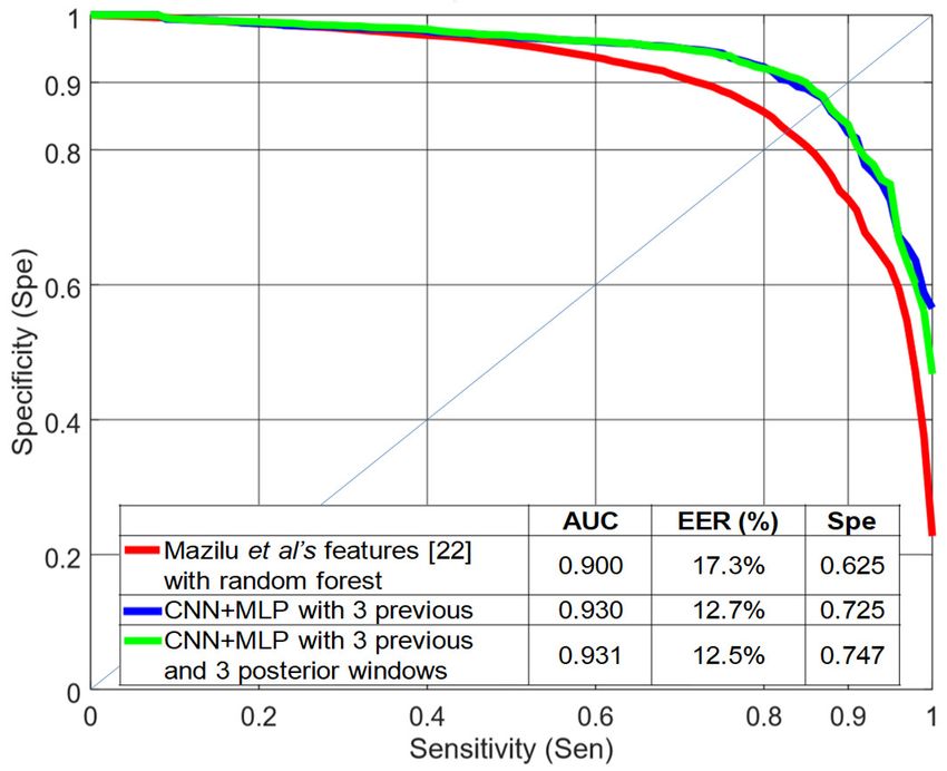
Electronics 2019, 8, 119                                                                                        5 of 15

two features. Lower autocorrelation values can be observed during FOG episodes. The second
quality metric was signal predictability. This metric, which tries to measure how easy is to predict
the signal using a linear model, was calculated by applying a linear prediction model with three
coefficients and computing the error between the real signal and the prediction, both in time and
frequency domains, generating two features. Higher errors are expected when FOG occurs. Finally,
the spectral flux was computed as the Euclidean distance between two normalized consecutive
window spectrums. A higher spectral flux can be observed when a FOG event starts. A total of five
features per signal (5 × 9 signals) were included in this feature set.

                               Table 1. Summary of the four feature sets used in this study.

                            Number of
  Feature set              features per                                  Description
                              signal
                                             Signal mean, standard deviation, variance, frequency entropy,
 Mazilu et al.
                                7            energy, freeze index (power of the freeze band (3–8 Hz) divided by
    [22]
                                             power in locomotor band (0.5–3 Hz)), and power in both bands.
                                             Time domain
                                             Signal mean value, standard deviation, median absolute deviation,
                                             largest value, smallest value, signal magnitude area, energy,
    Human                                    interquartile range, ecdf, entropy, auto regression coefficients, and
    activity                                 the correlation coefficient between two axes.
                               90
  recognition                                Frequency domain
  (HAR) [24]                                 Those considered in the time domain, and frequency with largest
                                             magnitude (in a 64-bin fast Fourier transform (FFT)), power,
                                             weighted average, skewness, kurtosis, and the energy of six
                                             equally spaced frequency bands.
Mel frequency
    cepstral
                               12            Mel frequency cepstral coefficients adapted to inertial signals.
  coefficients
 (MFCCs) [25]
Speech quality
                                             Harmonicity in time and frequency domains, predictability in time
  assessment                    5
                                             and frequency domains, and spectral flux.
(SQA) metrics

                                      Layer 1              Layer 2           Layer 3            3 Layers with
                                    32 × 9 × 128         32 × 3 × 42      1024 × 1 × 38         128, 32 and 1
        Input
                                                                                                   output
       9 × 128

                                                                                                   full connection
                5 × 5 convolution                             3×3           3 × 5 convolution
                   (32 kernels)                             Maxpooling         (32 kernels)

               Figure 2. Deep learning structure including convolutional and fully connected layers.

3.4. Classification Algorithms
     We analyzed several classification algorithms: random forest (baseline) with 100 decision trees,
a multilayer perceptron with three fully connected layers, and five-state hidden Markov models.
Additionally, a deep neural network was evaluated. This deep neural network was composed of six
layers (Figure 2) organized in two parts: the first part included two convolutional layers with an
intermediate maxpooling layer for feature extraction, and the second part integrated three fully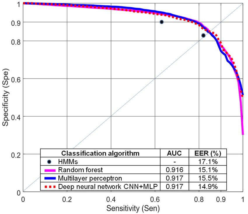
Electronics 2019, 8, 119                                                                             6 of 15

connected layers for classification (CNN + MLP). The inputs were the nine spectra (one for every
accelerometer signal and direction) with 128 points each. In the first and second convolutional
layers, 32 5 × 5 filters and 32 3 × 5 filters were considered, respectively. The configuration that
achieved the best performance in the training set (using part of the training set for validation) was
three epochs, batch size equal to 50, and ReLU as the activation function in all layers except the
output layer that used a sigmoid function instead. The loss function was the binary cross entropy
and the optimizer was the root-mean-square propagation method [27].

4. Experiments
      The majority of the experiments in this work were carried out with a LOSO cross validation. We
created the training set including sessions from all subjects except the one used for testing. This
process was iterated several times using a different subject for testing in each experiment. The final
results were computed by averaging all the experiments. In order to create baseline performance
numbers, we used a random 10-fold cross validation (R10Fold) for each subject independently. This
evaluation methodology was used in Mazilu et al. [22]. In this methodology, the sessions from every
subject were randomly divided into 10 folds; 9 folds were used for training and 1 for testing. The
process was repeated 10 times for each subject and the results were averaged. Only data from one
subject was used. The final results were computed by averaging across the subjects included in the
study. We computed specificity (true negative rate, the ratio of negatives that are correctly
identified) versus sensitivity (true positive rate, the ratio of positives that are correctly identified)
curves to compare the performance. These measurements are the most common metrics used in
human sensing studies. We also calculated F1-score, area under the curve (AUC), and equal error
rate (EER) in some experiments for an additional comparison.

4.1. Baseline and Comparison with Previous Work
       The best results on the Daphnet dataset were reported by Mazilu et al. [22]. The authors used
seven features extracted from each acceleration signal: signal mean, standard deviation, variance,
frequency entropy, energy, the ratio of the power in the freeze band to that in the locomotor band
(i.e., the freeze index), and the power in both bands individually. Mazilu et al. [22] compared several
ML algorithms and reported that the best results were with the random forest algorithm. They also
reported experiments with different window sizes in order to evaluate different latencies when
detecting FOG events. They achieved a sensitivity, specificity, and F1-score of 0.995, 0.999, and 0.998,
respectively, for their R10Fold experiments using a 4-s window. With LOSO evaluation, the
sensitivity and specificity decreased to 0.663 and 0.954, respectively.
       Most results in the literature used R10Fold evaluation rather than the more rigorous
LOSO evaluation. R10Fold validation, with overlapped windows, is a weak evaluation because
consecutive windows share data. Therefore, when the windows are shuffled before computing the
folds, there is a high probability that windows in training and testing sets include some of the same
raw data (Figure 3). Some of the previous results in the literature did not report the overlap when
using the R10Fold evaluation [22]. Others proposed alternatives for dividing the 10 folds in a
manner that avoids the inclusion of the same data in training and testing [18]. For comparison with
previous studies, we did some experiments using R10Fold with 4-s windows without excluding
subjects 4 and 10 and considering several overlaps. Table 2 shows that Mazilu and colleagues’
results [22] could be reproduced only with a significant overlap.

      Figure 3. Example of random assignment to train or test in a sequence of 50%-overlapped windows.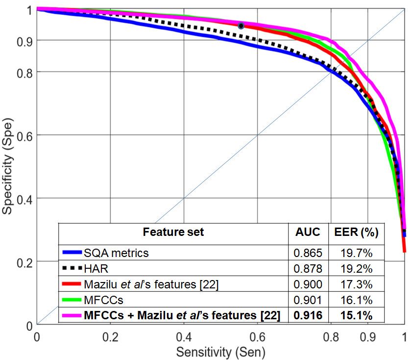
Electronics 2019, 8, 119                                                                                    7 of 15

      Table 2. Sensitivity, specificity, and F1-score varying amount of overlap for 4-s windows using
      R10Fold evaluation with all subjects.

 Overlap           Sensitivity    Specificity      F1-score                      System
 Unknown             0.995          0.999           0.998                    Mazilu et al. [22]
   90%               0.995          0.998           0.998        Ours (reproducing Mazilu et al.’s system)
   75%               0.934          0.939           0.961        Ours (reproducing Mazilu et al.’s system)
   50%               0.923          0.928           0.948        Ours (reproducing Mazilu et al.’s system)
   50%               0.915          0.915              -                    Alsheikh et al. [19]
   50%               0.820          0.820           0.830                  Hammerla et al. [17]
   0%                0.910          0.915           0.931        Ours (reproducing Mazilu et al.’s system)
   0%                0.719          0.967              -                      Ravi et al. [23]

     The use of a single value metric for evaluating performance, such as sensitivity, specificity,
accuracy, or F1-score, is problematic. These single value metrics depend on the threshold used by
the classifier to make a decision, increasing the difficulty of comparing different systems.
Additionally, some metrics (such as accuracy) have a strong dependency on the class balance in the
testing dataset. In the Daphnet dataset, less than 10% of the data pertains to FOG episodes (positive
examples), while the rest contains normal walking (negative examples), so classifying all examples
as negative gives an accuracy higher than 90%. In this paper, we used specificity and sensitivity
because these metrics do not depend on the class balance in testing.

4.2. Evaluation of the Different Feature Extraction Strategies
     Figure 4 compares several feature sets using a random forest classifier with 4-s windows and
75% overlap. Figure 4 shows specificity vs. sensitivity curves and AUC and EER values, all
computed using R10Fold cross validation. HAR and Mazilu et al.’s [22] feature sets performed better
than MFCCs in this evaluation. The quality metrics (blue line) provided an intermediate level of
performance. Mazilu et al.’s features, with only seven values per signal, obtained similar results
compared to the HAR feature set with 90 features per signal.

      Figure 4. Specificity vs. sensitivity curves, area under the curve (AUC), and equal error rate (EER) for
      the four sets of features, using random forest with 4-s windows and 75% overlap, a random 10-fold
      cross validation (R10Fold) evaluation, and excluding subjects 4 and 10.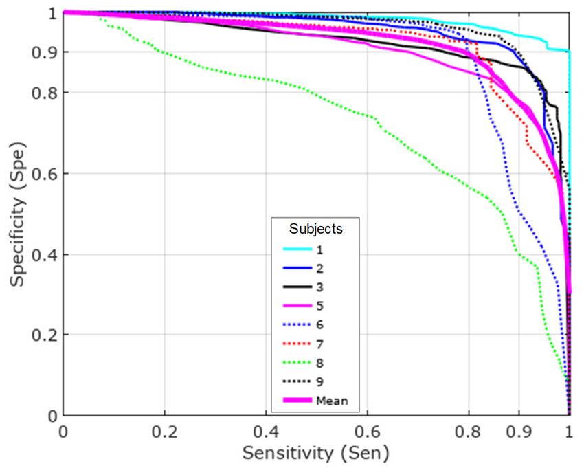
Electronics 2019, 8, 119                                                                                     8 of 15

      Figure 5. Results for Mazilu et al.’s features [22] (curves) for each subject compared to [13] when
      using optimized thresholds and R10Fold evaluation.

      When we compared the results per subject using Mazilu et al.’s [22] features with the results
reported by Bächlin et al. [13] (Figure 5), we saw an improvement in all subjects except for subject 1.
      Figure 6 compares the different feature sets with LOSO evaluation. MFCCs obtained slightly
better results than Mazilu et al.’s features. MFCCs create a smooth distribution (very similar to a
Gaussian distribution [28]) which is less likely to overfit and, therefore, has better generalization
behavior. HAR and quality metrics provided the worst results: they fit the data well in the R10Fold
experiment but were not able to generalize to held-out subjects. The best results were obtained when
combining Mazilu et al.’s [22] and MFCC features (concatenating the two feature vectors). Mazilu et
al. [22] reported a sensitivity of 0.66 and a specificity of 0.95, but these values included subjects 4 and
10, each of whom were associated with a sensitivity of 1.0. Removing these two subjects, the
sensitivity decreased to 0.55 for a specificity of 0.95 (isolated point in Figure 6).

      Figure 6. Specificity vs. sensitivity curves, AUC, and EER for the four sets of features using random
      forest with 4-s windows and 75% overlap, a leave-one-subject-out (LOSO) evaluation, and excluding
      subjects 4 and 10. The isolated point shows the results reported in Mazilu et al. [22] without subjects 4
      and 10 (sensitivity = 0.55 and specificity = 0.95).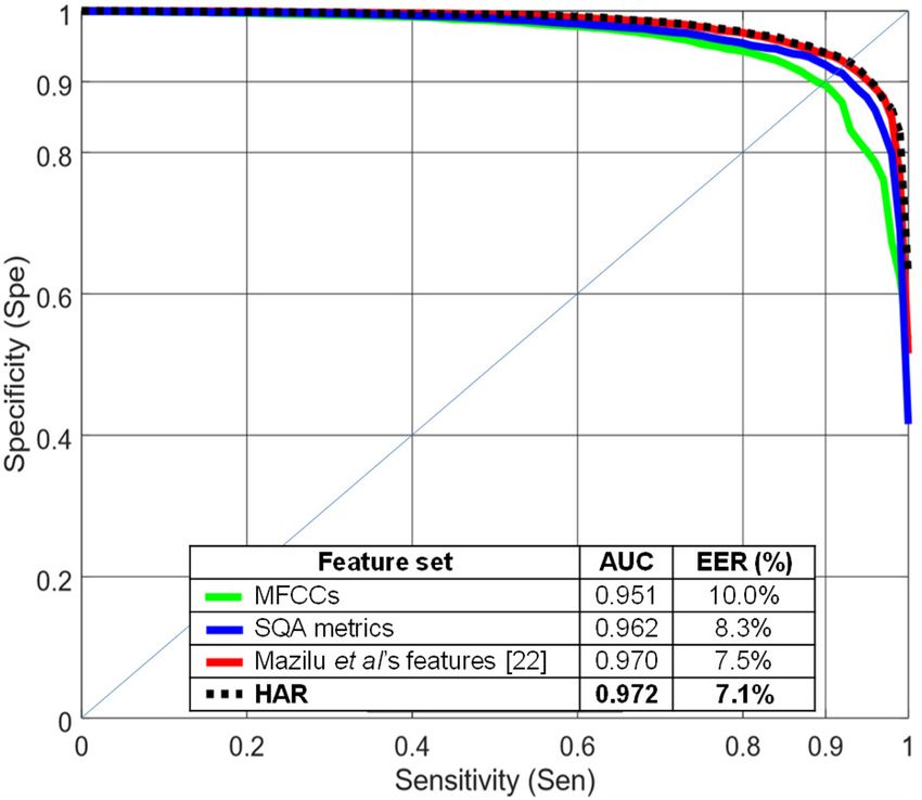
Electronics 2019, 8, 119                                                                            9 of 15

      Figure 7. Results per subject for MFCCs and Mazilu et al.’s features using a LOSO evaluation and
      excluding subjects 4 and 10.

     Figure 7 shows the results per subject using MFCCs and Mazilu et al.’s features together.
Subject 8 provided the worst results. This subject had many FOG events with a different pattern than
the other subjects, showing no increase in energy in the 3−8-Hz band. This unique pattern produced
bad results in a LOSO scenario, as it did not appear sufficiently in the training set.

4.3. Evaluation of Different Classification Algorithms
      We tested four different classification algorithms: random forest, multilayer perceptron, and
hidden Markov models (Figure 8), using MFCCs and Mazilu et al.’s features, and the deep neural
network described in Section 3.3. The performance of the HMMs is represented with two isolated
points corresponding to different probabilities for the transitions between FOG and
non-FOG HMMs. Hidden Markov models are finite state machines. Every time t that a state j is
entered, a feature vector Ot is generated from the probability density bj(Ot). The transition from state
i to state j is also probabilistic and modeled by the discrete probability aij. Figure 9 shows an example
of this process where the five-state model moves through the state sequence X = 1; 2; 3; 3; 4; 5; 5 in
order to generate the feature vector sequence O1 to O7. The weakest results were obtained with
HMMs. The HMMs required defining a sequential model with five states to achieve reasonable
discrimination. Therefore, a minimum number of windows (five windows corresponding to 5 s) was
necessary to make a decision. Short FOG episodes were missed when they appeared in isolation, or
consecutive FOG episodes were combined if the time between them was shorter than 5 s. In this
dataset, more than 30% of the FOG episodes lasted less than 5 s.
      The results obtained with random forest and multilayer perceptron were very similar and
better than HMMs. Both classifiers are discriminative algorithms using the same set of features. We
obtained slightly lower EER for the deep neural network.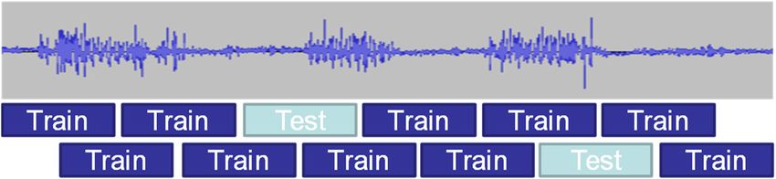
Electronics 2019, 8, 119                                                                                          10 of 15

      Figure 8. Specificity vs. sensitivity curves, AUC, and EER for the four classification algorithms with
      LOSO evaluation and excluding subjects 4 and 10. The two isolated points represent the performance
      using hidden Markov models with different probability transition between FOG and non-FOG
      models.

                      Markov
                      Model              a11          a22            a33           a44         a55

                           aintput 1           a12           a23           a34           a45          a5 output
                                          1           2              3             4           5
                                                            b3(O3)
                                                                         b3(O4)                      b5(O7)

                    Observation
                     Sequence

                                         O1      O2         O3       O4           O5      O6         O7

                                       Figure 9. Structure of the hidden Markov models.

4.4. Using Contextual Windows
      In the time leading up to a FOG event, there is an initial phase where some of the FOG
characteristics appear [18]. With this idea in mind, we tested whether or not the inclusion of features
from adjacent time windows, referred to here as contextual windows, would improve classification
performance. The effect of including the contextual windows in the classification task was evaluated
for the deep learning strategy with LOSO evaluation (CNN+MLP in Figure 10). The results
improved when previous and subsequent windows were included in the analysis but were
saturated when using three previous and three subsequent 4-s windows with a 75% overlap. The
CNN filters were able to find patterns between the spectra of consecutive windows. We did not
obtain significant improvements when including contextual windows with MFCCs and Mazilu et
al.’s features and a random forest classifier.
Electronics 2019, 8, 119 11 of 15
Figure 10. Specificity vs. sensitivity curves, AUC, and EER when including previous and posterior
windows in the deep neural network, using a LOSO evaluation and excluding subjects 4 and 10.
Table 3. AUC and EER when including only previous windows in the deep neural network, using a
LOSO evaluation and excluding subjects 4 and 10.
Contextual windows AUC EER (%)
CNN+MLP 0.917 14.9%
CNN+MLP with 1 previous window 0.922 14.0%
CNN+MLP with 2 previous windows 0.928 13.4%
CNN+MLP with 3 previous windows 0.930 12.7%
When using subsequent windows, a 1 second delay in the system response was introduced for
each subsequent window included in the decision. In order to reduce this delay, we repeated the
experiments using only previous windows (Table 3). Although the results were slightly worse than
when both previous and subsequent windows were included, we achieved significant improvement
without increasing the system delay.
Table 4 shows the performance for independent sensors (ankle, knee, and back accelerometers)
when including only previous windows. With the knee accelerometer, the results were very similar
to the case of using the three sensors. The worst results were obtained when using only the back
accelerometer.
Table 4. AUC and EER for independent sensors (ankle, knee, and back) when including only
previous windows in the deep neural network, using a LOSO evaluation and excluding subjects 4
and 10.
Sensors AUC EER (%)
All three accelerometers 0.930 12.7%
Ankle accelerometer 0.925 14.4%
Knee accelerometer 0.930 12.9%
Back accelerometer 0.914 15.0%Electronics 2019, 8, 119 12 of 15
Figure 11. Specificity vs. sensitivity curves, AUC, EER, and specificity (Spe) for a sensitivity of 0.95
when comparing the baseline and the best system in this paper with a LOSO evaluation and
excluding subjects 4 and 10.
Figure 11 shows a comparison between the baseline (Mazilu et al.’s features [22] with random
forest) and the best system obtained in this paper (CNN+MLP with three previous and three
subsequent windows) using a LOSO evaluation. This figure also includes the results for the
CNN+MLP structure when including only three previous windows. The EER decreased from 17.3%
to 12.5% and the AUC increased from 0.900 to 0.931. With this dataset, a difference of 0.015 (1.5%) in
AUC can be considered significant with p < 0.0005, according to Hanley’s method [29]. For high
levels of sensitivity (0.95), the specificity increased more than 0.12 when using previous and
subsequent windows and more than 0.10 when using only previous windows.
5. Discussion and Conclusions
We evaluated the robustness of different feature sets and ML algorithms for FOG detection
using body-worn accelerometers. The evaluation was carried out with subjects whose data was held
out from the training set (LOSO evaluation). We found that MFCCs were very good features in the
LOSO evaluation. The combination of the features proposed by Mazilu et al. [22] and MFCCs were
the best set of handcrafted features evaluated in this paper.
Hidden Markov models did not work well in this task because, in order to increase their
discrimination capability, the number of states had to be increased, losing resolution in the
segmentation process. The best results were obtained with a deep neural network that included two
convolutional layers combined with a maxpooling layer (for extracting features from the
accelerometer signal spectra) and three fully connected layers for classification. We obtained a
further improvement when we included temporal information in the detection process via
contextual windows. When comparing Mazilu et al.’s system [22] with our best system, the EER
decreased from 17.3% to 12.5% and the AUC increased from 0.900 to 0.931, obtaining the best results
for this dataset with a LOSO evaluation. Regarding the sensor placement, when using only the knee
accelerometer, the performance was very close to the case of using the three accelerometers.
A FOG detection system can be used to activate external cues, such as rhythmic acoustic ones.
These cueing systems help the patient to maintain a certain speed and amplitude of movements
when walking, reducing the duration and frequency of FOG episodes. These cues are more effective
when applied only during FOG episodes or in difficult walking situations. Therefore, FOG event
detection must have a high sensitivity (true positive rate) in order to activate the cueing system. For
high levels of sensitivity (95%), our best system increased the specificity from 0.63 to 0.73 without
adding delays to the detection process.Electronics 2019, 8, 119 13 of 15
The main characteristic of FOG is a significant power increment in the 3−8 Hz band. However,
the FOG pattern varies across subjects. For example, for subject 8, some FOG episodes did not show
an increase in power in the 3−8-Hz band. Differences among subjects present a challenge for a
system that must maintain high accuracy for unseen subjects. For future work, we would like to
validate these results using a larger number of subjects to deal with FOG variability across subjects.
With more data from a larger subject pool, it might be possible to train more complex deep learning
models and achieve better performance. Moreover, we could analyze different FOG patterns in
order to define distinct classes of this symptom that might help in designing better detection
systems.
Author Contributions: R.S.-S., H.N.-H., R.T.-S., and J.H. conceptualized the idea and defined the methodology.
R.S.-S., H.N.-H., and R.T. implemented the algorithms and ran the experiments. F.D.l.T. and J.H. performed the
formal analysis and obtained the funding required for the project. All authors contributed to writing,
reviewing, and editing the paper. All authors reviewed the manuscript.
Funding: This material is based upon work supported by the National Science Foundation under Grant No.
1602337. Ruben San Segundo’s internship at Carnegie Mellon University (CMU) has been supported by
Ministerio de Educación, Cultura y Deporte and the Fulbright Commission in Spain (PRX16/00103).
Acknowledgments: The authors would like to thank Andrew Whitford for proofreading the paper.
Conflicts of Interest: The authors declare no conflict of interest.
References
1. The 2015 Ageing Report. European Economy; European Commision: Brussels, Belgium, 2015, ISSN 0379-0991.
2. Pavón, J.; Gómez-Sanz, J.; Fernández-Caballero, A.; Valencia-Jiménez, J. Development of intelligent
multisensor surveillance systems with agents. Robot. Auton. Sys. 2007, 55, 892–903,
doi:10.1016/j.robot.2007.07.009.
3. Sama, A.; Perez-Lopez, C.; Romagosa, J.; Rodriguez-Martin, D.; Catala, A.; Cabestany, J.; Perez-Martinez,
D.; Rodriguez-Molinero, A. Dyskinesia and Motor State Detection in Parkinson’s Disease Patients with a
Single Movement Sensor. In Proceedings of the Annual International Conference of the IEEE Engineering
in Medicine and Biology Society, San Diego, CA, USA, 28 August–21 September 2012; pp. 1194–1197,
doi:10.1109/EMBC.2012.6346150.
4. Herrlich, S.; Spieth, S.; Nouna, R.; Zengerle, R.; Giannola, L.; Pardo-Ayala, D.E.; Federico, E.; Garino, P.
Ambulatory Treatment and Telemonitoring of Patients with Parkinsons Disease. In Ambient Assisted
Living; Springer: Berlin/Heidelrberg, 2011, doi:10.1007/978-3-642-18167-2_20.
5. Moore, O.; Peretz, C.; Giladi, N. Freezing of gait affects quality of life of peoples with Parkinson’s disease
beyond its relationships with mobility and gait. Mov. Disord. 2007, 22, 2192–2195, doi:10.1002/mds.21659.
6. Nutt, G.; Bloem, B.R.; Giladi, N.; Hallett, M.; Horak, F.B.; Nieuwboer, A. Freezing of gait: Moving forward
on a mysterious clinical phenomenon. Lancet Neurol. 2011, 10, 734–744, doi:10.1016/S1474-4422(11)70143-0.
7. Schaafsma, D.; Balash, Y.; Gurevich, T.; Bartels, A.L.; Hausdorff. M.; Giladi, N. Characterization of freezing
of gait subtypes and the response of each to levodopa in Parkinson’s disease. Eur. J. Neurol. 2003, 10,
391–398, doi:10.1046/j.1468-1331.2003.00611.x.
8. Arias, P.; Cudeiro. J. Effect of rhythmic auditory stimulation on gait in parkinsonian patients with and
without freezing of gait. PLoS ONE 2010, 5, e9675, doi:10.1371/journal.pone.0009675.
9. Young, W.R.; Shreve, L.; Quinn, E.J.; Craig, C.; Bronte-Stewart H. Auditory cueing in Parkinson’s patients
with freezing of gait. What matters most: Action-relevance or cue-continuity? Neuropsychologia 2016, 87,
54–62, doi:10.1016/j.neuropsychologia.2016.04.034.
10. Goetz, C.G.; Tilley, B.C.; Shaftman, S.R.; Stebbins, G.T.; Fahn, S.; Martinez Martin, P.; Poewe, W.; Sampaio,
C.; Stern, M.B.; Dodel, R.; et al., Movement disorder society-sponsored revision of the unified Parkinson’s
disease rating scale (mds-updrs): Scale presentation and clinimetric testing results Mov. Disord. 2008, 23,
2129–2170, doi:10.1002/mds.22340.
11. Richard, H.I.; Frank, S.; LaDonna, K.A.; Wang, H.; McDermott, M.P.; Kurlan, R. Mood fluctuations in
Parkinson’s disease: A pilot study comparing the effects of intravenous and oral levodopa administration.
Neuropsychiatr. Dis. Treat. 2005, 1, 261–268.Electronics 2019, 8, 119 14 of 15
12. Available online:
http://parkinsonslife.eu/more-than-a-third-of-parkinsons-patients-hide-symptoms-out-of-fear-or-shame/
(accessed on 20 January 2019).
13. Bächlin, M.; Plotnik, M.; Roggen, D.; Maidan, I.; Hausdorff, J.M.; Giladi, N.; Träster, G. Wearable assistant
for Parkinson’s disease patients with the freezing of gait symptom. IEEE Trans. Inf. Technol. Biomed. 2010,
14, 436–446, doi:10.1109/TITB.2009.2036165.
14. Yi, X.; Qingwei, G.; Qiang, Y. Classification of gait rhythm signals between patients with
neuro-degenerative diseases and normal subjects: Experiments with statistical features and different
classification models. Biomed. Signal Process. Control 2015, 18, 254–262, doi:10.1016/j.bspc.2015.02.002.
15. Su, B.L.; Song, R.; Guo, L.Y.; Yen, C.W. Characterizing gait asymmetry via frequency sub-band
components of the ground reaction force. Biomed. Signal Process. Control 2015, 18, 56–60,
doi:10.1016/j.bspc.2014.11.008.
16. Wu, Y.; Chen, P.; Luo, X.; Wu, M.; Liao, L.; Yang, S.; Rangayyan, R.M. Measuring signal fluctuations in gait
rhythm time series of patients with Parkinson’s disease using entropy parameters. Biomed. Signal Process.
Control 2017, 31, 265–271, doi:10.1016/j.bspc.2016.08.022.
17. Hammerla, N.; Kirkham, R.; Andras, P.; Ploetz, T. On Preserving Statistical Characteristics of
Accelerometry Data using their Empirical Cumulative Distribution. ISWC ‘13 In Proceedings of the 2013
International Symposium on Wearable Computers, Zurich, Switzerland, 8–12 September 2013; pp. 65–68,
doi:10.1145/2493988.2494353.
18. Mazilu, S.; Calatroni, A.; Gazit, E.; Roggen, D.; Hausdorff, J.M.; Tröster, G. Feature Learning for Detection
and Prediction of Freezing of Gait in Parkinson’s Disease. In Proceedings of the International Workshop
on Machine Learning and Data Mining in Pattern Recognition. MLDM: Machine Learning and Data
Mining in Pattern Recognition, New York, NY, USA, 19–25, 2013; pp 144–158, doi:10.1155/2012/459321.
19. Alsheikh, M.A.; Selim, A.; Niyato, D.; Doyle, L.; Lin, S.; Tan, H.P. Deep Activity Recognition Models with
Triaxial Accelerometers. In Proceedings of the Workshops of the Thirtieth AAAI Conference on Artificial
Intelligence, Phoenix, AZ, USA, 12–13 February 2016.
20. Moore, S.T.; MacDougall, H.G.; Ondo, W.G. Ambulatory monitoring of freezing of gait in Parkinson’s
disease. J. Neurosci. Methods 2008, 167, 340–348, doi:10.1016/j.jneumeth.2007.08.023.
21. Assam, R.; Seidl, T. Prediction of Freezing of Gait from Parkinson’s Disease Movement Time Series using
Conditional Random Fields. In Proceedings of the Third ACM SIGSPATIAL International Workshop on
the Use of GIS in Public Health, HealthGIS, Dallas, TX, USA, 4 November 2014,
doi:10.1145/2676629.2676630.
22. Mazilu, S., Hardegger, M., Zhu, Z., Roggen, D., Tröster, G., Plotnik, M., Hausdorff, J. Online Detection of
Freezing of Gait with Smartphones and Machine Learning Techniques. In Proceedings of the 6th
International Conference on Pervasive Computing Technologies for Healthcare, San Diego, CA, USA,
21–24 May 2012, doi:10.4108/icst.pervasivehealth.2012.248680
23. Ravì; D; Wong, C.; Lo, B.; Yang, G.Z. Deep Learning for Human Activity Recognition: A Resource Efficient
Implementation on Low-Power Devices. In Proceedings of the 2016 IEEE 13th International Conference on
Wearable and Implantable Body Sensor Networks (BSN), San Francisco, CA, USA, 14–17 June 2016,
doi:10.1109/BSN.2016.7516235.
24. San-Segundo, R.; Lorenzo-Trueba, J.; Martínez-González, B.; Pardo, J.M. Segmenting human activities
based on HMMs using smartphone inertial sensors. Pervasive Mobile Comput. 2016 30, 84–96,
doi:10.1016/j.pmcj.2016.01.004.
25. San-Segundo, R.; Montero, J.M.; Barra-Chicote, R.; Fernandez, F.; Pardo, J.M. Frequency extraction from
smartphone inertial signals for human activity segmentation. Signal Process. 2016, 120, 359–372,
doi:10.1016/j.sigpro.2015.09.029.
26. Raake, A. Speech Quality of VoIP: Assessment and Prediction; John Wiley & Sons Ltd.: Hoboken, NJ, USA.
27. Tieleman, T.; Hinton, G. Lecture 6.5-rmsprop: Divide the gradient by running average of its recent
magnitude. COURSERA: Neural Networks for Machine Learning. Available online:
https://en.coursera.org/learn/neural-networks-deep-learning (accessed on 20 January 2019)
28. San-Segundo, R.; Blunck, H.; Moreno-Pimentel, J.; Stisen, A.; Gil-Martín, M., Robust human activity
recognition using smartwatches and smartphones. Eng. Appl. Artif. Intell. 2018, 72, 190–202,
doi:10.1016/j.engappai.2018.04.002.Electronics 2019, 8, 119 15 of 15
29. Hanley, J.A.; McNeil, B.J. The meaning and use of the area under a receiver operating characteristic (ROC)
curve. Radiology 1982, 143, 29–36.
© 2019 by the authors. Licensee MDPI, Basel, Switzerland. This article is an open access
article distributed under the terms and conditions of the Creative Commons Attribution
(CC BY) license (http://creativecommons.org/licenses/by/4.0/).You can also read